BAYESIAN INFERENCE AND PREDICTION FOR NORMAL
DISTRIBUTION BASED ON RECORDS
Akbar Asgharzadeh1
Department of Statistics, Faculty of Mathematical Sciences, University of Mazandaran, Babolsar, Iran Reza Valiollahi
Department of Statistics, Statistics and Computer Science, Semnan University, Semnan, Iran Adeleh Fallah
Department of Statistics, Payame Noor University, P. O. Box 19395-3697, Tehran, Iran Saralees Nadarajah
School of Mathematics, University of Manchester, Manchester M13 9PL, UK
1. INTRODUCTION
LetX1,X2, . . . be independent and identical random variables with the cumulative dis-tribution function (cdf)F(x)and the probability density function (pdf) f(x). Define
Yn=max{X1, . . . ,Xn}
for n ≥ 1. Then,Xj is an upper record value of this sequence ifXj >Yj−1, j > 1. Generally, if we define the sequence{U(n),n≥1}as
U(1) =1, U(n) =min¦j:j>U(n−1),Xj>XU(n−1)©
for n ≥ 2, then¦XU(n),n≥1© is a sequence of upper record values. The sequence
{U(n),n≥1}represents the record times.
Chandler (1952) defined the theory of records as a model for successive extremes in a sequence of independent and identical random variables. Record data arise in many real life problems, such as in destructive stress testing, weather, hydrology, economics and sporting and athletic events. For more details and applications, see Ahsanullah (1995), Arnoldet al.(1998) and Nevzorov (2000).
In the frequentist set up, the estimation and prediction problems for normal dis-tribution based on record data have been discussed by several authors. Balakrishnan and Chan (1998) obtained the best linear unbiased estimators (BLUEs) of the normal location and scale parameters,µandσ, based on the first few upper record values. Us-ing these BLUEs, they then developed a prediction interval for a future record value. Chacko and Mary (2013) discussed classical estimation and prediction for the normal distribution based onk-records. Sajeevkumar and Irshad (2014) estimated the location parameter of distributions with known coefficient of variation by record values.
The main aim of this paper is to consider estimation and prediction for normal dis-tribution based on record data in the Bayesian set up. To the best of our knowledge, this problem has not been studied before in the literature. We compute Bayes estimators ofµ andσunder squared error and Linex loss functions. It is observed that Bayes estimators can not be obtained in closed forms. We use the importance sampling procedure to gen-erate samples from the posterior distributions and then compute the Bayes estimators. We then compare Bayes estimators with the maximum likelihood estimators (MLEs) and BLUEs by Monte Carlo simulations. We observe that Bayes estimators work quite well. Bayesian prediction of future records based on the first few upper records is also discussed. We use the importance sampling method to estimate the predictive distribu-tion and then compute the Bayesian predictors.
The contents of this paper are organized as follows. In Section 2, we provide a brief review of frequentist estimators and predictors. In Section 3, the Bayes estimators of
µandσ are obtained using squared error and Linex loss functions. In Section 4, we discuss Bayesian prediction for future records based on the first few upper records. In Section 5, a real data set is analyzed for illustrative purposes. Monte Carlo simulations are performed to compare the proposed estimators and predictors in Section 6. Finally, we conclude the paper in Section 7.
2. FREQUENTIST ESTIMATION AND PREDICTION: AREVIEW
Suppose that we observe the firstnupper record valuesXU(1)=x1,XU(2)=x2, . . . ,XU(n)
=xn from the normalN µ,σ2
distribution. For notational simplicity, we will write
Xi forXU(i). The likelihood function is given (see Arnoldet al., 1998) by
L(µ,σ|x) =f (xn;µ,σ) n−1
Y
i=1
f(xi;µ,σ) 1−F(xi;µ,σ),
where f(xn;µ,σ)andF(xn;µ,σ)denote, respectively, the pdf and cdf of theN µ,σ2
The likelihood function can be rewritten as
L(µ,σ|x) = σ1φ
x
n−µ
σ n−1 Y i=1 1 σφ x
i−µ
σ
1−Φx
i−µ
σ = 1 σ n n Y i=1 φ
xi−µ
σ
n−1
Y
i=1
1−Φ
xi−µ
σ
−1
, (1)
whereφ(·)andΦ(·)denote, respectively, the pdf and cdf of a standard normal distribu-tion.
The log-likelihood function is
L=lnL(µ,σ|x) =−nlnσ+
n
X
i=1 lnφ
x
i−µ
σ
−
n−1
X
i=1 ln
1−Φ x
i−µ
σ
. (2)
From (2), we obtain the likelihood equations forµandσas
∂L
∂ µ=
1
σ2 n
X
i=1
(xi−µ)−σ1
n−1
X
i=1 φx
i−µ
σ
1−Φxi−µ
σ
=0 (3)
and
∂L
∂ σ =−
n σ+ 1 σ3 n X i=1
(xi−µ)2−σ12
n−1
X
i=1
(xi−µ)φxi−µ
σ
1−Φx
i−µ
σ
=0. (4)
The equations (3) and (4) can be solved analytically to obtainµbM LandσbM L, the MLEs
ofµandσ.
Following the generalized least-squares approach, the BLUEs ofµandσcan be de-rived as (see Balakrishnan and Cohen, 1991)
b
µB LU=Xn
i=1
aiXi, σbB LU=
n
X
i=1
biXi, (5)
where
a= α
0β−1α10β−1−α0β−11α0β−1 (α0β−1α)(10β−11)−(α0β−11)2
and
b= 1
whereα0 = (α
1,α2, . . . ,αn)is the moment vector withαi = E(Xi)and β=
βi,j
,
1≤i≤j≤nis the covariance matrix withβi,j=CovXi,Xj, and10= (1, 1, . . . , 1) 1×n. The variances of these BLUEs are given by
Var(µbB LU) =
α0β−1α
(α0β−1α)(10β−11)−(α0β−11)2
σ2=V
1σ2
and
Var(σbB LU) =
10β−11
(α0β−1α)(10β−11)−(α0β−11)2
σ2=V
2σ2.
The coefficientsa,band the values ofV1andV2can be found in Balakrishnan and Chan (1998, Tables 3 to 5). See also Arnoldet al.(1998, Table 5.3.1, pages 139 and 140). From
those tables, we can see that n
X
i=1
ai=1 and n
X
i=1
bi=0.
By using the BLUEs, one can construct confidence intervals (CIs) for the location and scale parameters,µandσ, through pivotal quantities given by
R1= µbB LU−µ
b σB LUp
V1, R2=
b σB LU−σ
b σB LUp
V2. (6)
For constructing such CIs, we require the percentage points ofR1andR2, which can be computed by using the BLUEsµbB LU andσbB LU via Monte Carlo simulations. Table 1 gives the percentage points ofR1andR2based on ten thousand replications and different choices ofn. The following algorithm was used to determine the percentage points:
1. set a value forn;
2. simulateXU(1),XU(2), . . . ,XU(n)from a standard normal distribution;
3. computeµbB LUandσbB LU from (5);
4. then computeR1andR2from (6) by takingµ=0 andσ=1;
5. repeat steps 2 to 4 ten thousand times, obtaining ten thousand estimates forR1
and ten thousand estimates forR2;
6. compute the percentage points ofR1as the quantiles of the empirical distribution of the ten thousand estimates ofR1;
LetR1(α)andR2(α)denote the percentage points atαdetermined through simulation for the pivotal quantitiesR1andR2, respectively. Then,
b
µB LU−σbB LUR1(1−α/2) p
V1,µbB LU−σbB LUR1(α/2) p
V1
and
b
σB LU−σbB LUR2(1−α/2) p
V2,σbB LU−σbB LUR2(α/2) p
V2
form 100(1−α)percent CIs forµandσ based on the pivotal quantitiesR1and R2, respectively.
Note that if we defineY = XU(n+1) as the next upper record value, then we can predict this value by using the best linear unbiased prediction (BLUP) method. The BLUP of the next upper record value can be derived as (see Balakrishnan and Chan, 1998)
Ò
YB LU P =µbB LU+σbB LUαn+1.
TABLE 1
Simulated percentage points of R1and R2.
Percentage points ofR1.
n 1% 2.5% 5% 10% 90% 95% 97.5% 99%
2 -4.318 -2.765 -1.766 -1.165 2.975 4.926 7.187 9.945 3 -2.240 -1.633 -1.292 -1.003 2.587 3.970 5.662 8.125 4 -1.706 -1.430 -1.223 -0.997 2.253 3.506 4.906 6.795 5 -1.704 -1.443 -1.240 -0.999 2.038 3.107 4.193 5.974 6 -1.592 -1.375 -1.185 -0.944 2.140 3.136 4.218 5.572 7 -1.598 -1.390 -1.224 -1.030 1.825 2.776 3.778 4.930 8 -1.653 -1.441 -1.254 -1.033 1.876 2.717 3.542 4.709 9 -1.664 -1.442 -1.281 -1.048 1.767 2.548 3.384 4.368 10 -1.631 -1.453 -1.264 -1.045 1.740 2.439 3.219 4.222
Percentage points ofR2.
n 1% 2.5% 5% 10% 90% 95% 97.5% 99%
3. BAYES ESTIMATION
In Bayesian inference, a loss functionLθ,θb
describes the loss incurred by making an
estimateθbwhen the true value of the parameter isθ. Here, we consider two different
loss functions: first is the squared error loss function which is symmetric and second is the linear-exponential (Linex) loss function which is an asymmetric function. In the literature, the most commonly used loss function is the squared error. The symmetric nature of this function gives equal weight to overestimation as well as underestimation. However, for many situations, overestimation may be more serious than underestima-tion or vice-versa (see, for example, Feynman, 1987). Therefore, in order to make statis-tical inferences more pracstatis-tical and applicable, we often need to choose an asymmetric loss function. Many authors have considered asymmetric loss functions in reliability and life testing. See, for example, Basu and Ebrahimi (1991), Ahmadiet al.(2005), Ren
et al.(2006), Raqabet al.(2007), Soliman and Al-Aboud (2008), Asgharzadeh and Fallah
(2011), Kundu and Raqab (2012), Asgharzadehet al.(2015).
One of the most popular asymmetric loss function is the Linex loss function
Lθ,θb
=ec
b
θ−θ
−cθb−θ
−1, (7)
wherec6=0. This loss function was introduced by Varrian (1975) and was extensively discussed by Zellner (1986). The sign and magnitude of the shape parametercrepresents the direction and degree of asymmetry, respectively. Ifc>0, overestimation is more serious than underestimation, and vice-versa. Whencis close to zero,
Lθ,θb
=X∞
k=0
ck b θ−θk
k! −c
b
θ−θ−1= ∞
X
k=2
ck b θ−θk
k! ≈
c2 2
b θ−θ2.
Hence, whencis close to zero, the Linex loss is approximately equal to the squared error loss and therefore almost symmetric.
The posterior expectation of the Linex loss function (7) is
EθLθ,θb
=ecθb
Eθe−cθ−cθb−Eθ(θ)
−1, (8)
whereEθ(·)denotes the posterior expectation with respect to the posterior pdf ofθ. The Bayes estimator ofθunder the Linex loss function, denoted byθb
B L, is the value of
b
θwhich minimizes (8). It is
b θB L=−
1
cln
¦
Eθe−cθ©,
provided that the expectationEθ[exp(−cθ)]exists and is finite.
joint prior pdf as a product of a conditional pdf ofµfor givenσ(which is taken to be theN µ0,σ2
pdf, whereµ0∈ ℜis known) and a square-root inverted-gamma pdf for
σwhich has the form
π(σ) = ab
Γ(b)2b−1σ
−2b−1exp
− a
2σ2
, (9)
whereσ >0,a>0 andb >0. Note that the choice of a square-root inverted-gamma prior forσis equivalent to selecting a gamma prior forλ=1/σ2. An improper prior forσisπ(σ)∝σ−1(An improper prior is one that does not integrate to 1. There are no unique improper priors for a given prior. For the prior in (9), there are uncountably infinite ways of defining improper priors. The improper priors need not be particular cases of (9).) For more details on the square-root inverted-gamma distribution, see Raqab and Madi (2002), Wuet al.(2006) and Soliman and Al-Aboud (2008).
So, the joint prior pdf ofµandσcan be written as
π(µ,σ) =π(µ|σ)π(σ)∝σ−2b−2exp
−1 2σ2
a+ (µ−µ0)2
.
Now, by multiplying the likelihood function in (1) by the joint prior pdf, the poste-rior pdf ofµandσcan be derived as
π(µ,σ|x) ∝ σ−n−2b−2exp
−1 2σ2
(n−1)s2+n(x−µ)2
·exp
−1 2σ2
a+ (µ−µ0)2
h(µ,σ)
= σ−1exp
−n+1
2σ2
µ−nx+µ0
n+1
2
(10)
·σ−2(n2+b)−1exp
−1 2σ2
a+ (n−1)s2+n(x−µ0)
2
n+1
h(µ,σ),
where
x= 1
n
n
X
i=1
xi, s2= 1
n−1
n
X
i=1
(xi−x)2
and
h(µ,σ) =
n−1 Y
i=1
1−Φ x
i−µ
σ
−1
. (11)
The Bayes estimator of any function ofµandσ, sayk(µ,σ), under the squared error loss is
b
kB S(µ,σ) =Eπ[k(µ,σ)|x] =
Z∞
0
Z∞
−∞
whereEπ(·)denotes the expectation with respect to the joint posterior pdfπ(µ,σ|x)in (10). This can not be reduced to a closed form.
3.1. Importance sampling method
Here, we consider the importance sampling method to generate samples from the pos-terior distribution and then compute the Bayes estimators ofµandσunder the squared error and Linex loss functions.
Based on the joint posterior pdf ofµandσ, (10) can be written as
π(µ,σ|x)∝g1(µ|σ,x)g2(σ|x)h(µ,σ), (12)
whereg1(µ|σ,x)denotes a normal pdf with meannx+µ0
n+1 and variance
σ2
n+1. Alsog2(σ|x) denotes a square-root inverted-gamma pdf with shape parameter n2+band scale
param-eterha+ (n−1)s2+n(x−µ0)2 n+1
i
, andh(µ,σ)is given by (11).
Sinceg2(σ|x)is a square-root inverted-gamma pdf, it is simple to generateσ. Then, by using the generatedσ,µcan be simulated from g1(µ|σ,x)for a givenx. Now, sim-ilarly to Kundu and Pradhan (2009) and Kundu and Howlader (2010), we can use the importance sampling procedure to compute Bayes estimators. Using (12), the Bayes estimator ofk(µ,σ)can be written as
b
kB S(µ,σ) =Eπ[k(µ,σ)|x] =
Z∞
0
Z∞
−∞
k(µ,σ)h(µ,σ)g1(µ|σ,x) g2(σ|x)dµdσ
Z∞
0
Z∞
−∞
h(µ,σ)g1(µ|σ,x) g2(σ|x)dµdσ
= Eπ0[k(µ,σ)h(µ,σ)]
Eπ0[h(µ,σ)]
,
whereEπ0(·)denotes the expectation with respect to the joint pdf
π0(µ,σ|x) =g
1(µ|σ,x) g2(σ|x).
Now, the Bayes estimator ofk(µ,σ)can be approximated by
b
kB S(µ,σ) = 1
N
N
X
i=1
k(µi,σi)h(µi,σi)
1
N
N
X
i=1
h(µi,σi)
π0is referred to as the importance distribution. The distributionπis referred to as the nominal distribution.
Therefore, Bayes estimators can be computed using the following algorithm:
step 1. Generateσ1fromg2(σ|x)andµ1fromg1(µ|σ1,x).
step 2. Repeat step 1,N times to obtain(µ1,σ1), . . . ,(µN,σN).
step 3. Bayes estimators ofµandσunder the squared error loss function are
b µM C
B S = N
X
i=1
µiwi, σb
M C B S =
N
X
i=1 σiwi.
The estimators based on the Linex loss function are
b µM C
B L =− 1
cln
N X
i=1
e−cµiw
i
, σbM C
B L =− 1
cln
N X
i=1
e−cσiw
i
,
where
wj= h
µj,σj
PN j=1h
µj,σj
(13)
for j=1, 2, . . . ,N.
We implemented the above algorithm in the R software (R Development Core Team, 2016), using our own codes. The samples needed for construction of highest posterior density (HPD) credible intervals were also generated by using our own codes in the R software. All computational procedures for this paper were implemented using our own codes in the R software. None of the contributed packages in the R software were used.
3.2. HPD credible intervals
To construct HPD intervals, we use the Monte Carlo procedure proposed by Chen and Shao (1999). Given the Monte Carlo samplesµj,σj,j=1, 2, . . . ,N, we compute the HPD interval forµas follows:
Step 1. Sort¦µj,j=1, . . . ,N©as
µ(1)≤µ(2)≤ · · · ≤µ(N).
Step 2. Compute the 100(1−α)percent credible intervals
Li(N) =µe(
i N),
e µi+[(1N−α)N]
fori=1, 2, . . . ,N−[(1−α)N], where
e µ(γ)=
µ(1), ifγ=0,
µ(i), if i−1
X
j=1
wj< γ ≤
i
X
j=1
wj.
Here,[(1−α)N]denotes the integer part of(1−α)N.
Step 3. The 100(1−α)percent HPD interval is the one with the smallest interval width among allLi(N)’s.
The same procedure can be applied to calculate the HPD interval forσ.
4. BAYESIAN PREDICTION
Suppose that we observe only the n upper record observations XU(1) = x1,XU(2) = x2, . . . ,XU(n) = xn, and the aim is to predict thesth upper record value, s > n. Let
Y ≡XU(s)be thesth upper record value.
The conditional distribution ofY givenX = (x1,x2, . . . ,xn)is just the distribution ofY givenXU(n)=xn, due to the well-known Markovian property of record statistics. It follows (see Arnoldet al.(1998)) that
f(y|xn;µ,σ) =[H(y)−H(xn)] s−n−1 Γ(s−n)
f(y;µ,σ) 1−F(xn;µ,σ),
wherey>xnandH(y) =−ln[1−F(y)]. For the normal distribution, f(y|xn;µ,σ)is given by
f (y|xn;µ,σ) =
ln
1−Φxn−µ
σ
1−Φy−σµ
s−n−1
φy−µ σ
σΓ(s−n)1−Φxn−µ
σ .
The Bayes predictive pdf ofY, f∗
s (y|xn), can be calculated as
fs∗(y|xn) =
Z∞
0
Z∞
−∞
f (y|xn;µ,σ)π(µ,σ|x)dµdσ. (14)
Substituting (12) into (14), the Bayes predictive pdf f∗
s (y|xn)can be obtained as
fs∗(y|xn)∝ Z∞
0
Z∞
−∞
4.1. Bayesian point prediction
The Bayesian point predictors ofY under the squared error loss function,YÒSE P, and
under the Linex loss function,YÒLE P, are
Ò
YSE P=
Z∞
xn
y fs∗(y|xn)d y (15)
and
Ò
YLE P=−1
cln
Z∞ xn
e−c yfs∗(y|xn)
d y. (16)
Since fs∗(y|xn)can not be expressed in closed form, (15) and (16) can not computed explicitly. As before, based on the Monte Carlo sample{(µi,σi),i=1, 2, . . . ,M}, a sim-ulation consistent estimator of f∗
s (y|xn)can be obtained as
b
fs∗(y|xn) =
M
X
i=1
f (y|xn;µi,σi)wi, (17)
wherewi,i =1, 2, . . . ,N are as defined in (13). By using (17),YÒSE P andYÒLE P can be
computed as
Ò
YSE P=
Z∞
xn
y
M
X
i=1
f (y|xn;µi,σi)wid y=
M
X
i=1
wiI(xn,µi,σi)
and
Ò
YLE P=−1
cln
Z∞ xn
e−c y
M
X
i=1
f(y|xn;µi,σi)wid y
=−1
cln
M X
i=1
wiJ(xn,µi,σi)
,
where
I(xn,µ,σ) =
Z∞ xn y ln
1−Φxn−µ
σ
1−Φy−σµ
s−n−1
φy−µ σ
σΓ(s−n)1−Φxn−µ
σ d y
and
J(xn,µ,σ) =
Z∞
xn
e−c y
ln
1−Φxn−µ
σ
1−Φy−σµ
s−n−1
φy−µ σ
σΓ(s−n)1−Φxn−µ
4.2. Bayesian interval prediction
Bayesian prediction intervals can be obtained from the Bayes predictive pdf f∗(y|x). Bayesian prediction bounds can be obtained by evaluating
P(Y> λ|xn) =
Z∞
λ
fs∗(y|xn)d y
for some positiveλ. Now, the 100(1−α)percent Bayesian prediction interval forY is given by(L(x),U(x)), whereL(x)andU(x)can be obtained by solving the following non-linear equations simultaneously
P(Y>L(x)|xn) =
Z∞
L(x)
fs∗(y|xn)d y=1−α
2
and
P(Y>U(x)|xn) =
Z∞
U(x)
fs∗(y|xn)d y=α
2.
By substituting fb∗
s (y|xn)in (17) for fs∗(y|xn), we can obtain the Bayesian prediction boundsL(x)andU(x)from the following equations:
1−α
2 = M
X
i=1
wiK(L(x),µi,σi), α
2 = M
X
i=1
wiK(U(x),µi,σi),
where
K(L,µ,σ) =
Z∞
L
ln
1−Φx
n−µ
σ
1−Φy−σµ
s−n−1
φy−µ σ
σΓ(s−n)1−Φxn−µ
σ d y.
5. REAL DATA ANALYSIS
In this section, we consider a real data set to illustrate all the estimation and prediction methods described in the preceding sections. The data are the total annual rainfall in inches during March recorded at Los Angeles Civic Center from 1997 to 2006 (see the website of Los Angeles Almanac,www.laalman-ac.com/weather/we08aa.htm):
0.00, 4.06, 1.24, 2.82, 1.17, 0.32, 4.31, 1.17, 2.14, 2.87.
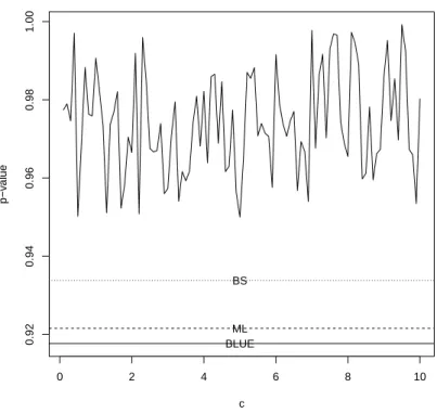
From this data, we observe the three upper record values as 0.00, 4.06, 4.31. For this record data, we estimatedµandσ using MLE, BLUE of Balakrishnan and Chan (1998) and Bayes estimators. For computing Bayes estimators and predictors, since we do not have any prior information, we assume that the prior onσis improper. Sinceµ0 is the location hyper parameter, without loss of generality, we assume thatµ0=0. The integralsI,J in Section 4.1 andKin Section 4.2 were computed numerically using the functionintegratein the R software (R Development Core Team, 2016).integrateis based on QUADPACK routinesdqagsanddqagiby R. Piessens and E. deDoncker-Kapenga, available from Netlib. The number of subdivisions for integration was taken to be 100. Figure 1 plots the p-value of the K-S test versuscwhen Bayes estimator is used with the Linex loss function. Also plotted are the p-values corresponding to the MLE, BLUE and Bayes estimator with the squared error loss function. We see that BLUE has the smallest p-value and MLE has the second smallest p-value. The p-values for Bayes esti-mators are larger. The asymmetric Linex loss always produces larger p-values than the squared error loss.
0 2 4 6 8 10
0.92
0.94
0.96
0.98
1.00
c
p−v
alue
BLUE ML BS
We also computed CIs forµandσ. The 95 percent HPD intervals using the Monte Carlo method were(1.95, 2.11)and(1.481, 1.500)forµandσ, respectively. The 95 per-cent CIs based on the BLUEs through the pivotal quantitiesR1andR2were(1.91, 2.22) and(1.476, 1.511)forµandσ, respectively. We see that the former intervals are shorter. All of the intervals contain the MLEs ofµandσbased on the complete sample (µ=2.01 andσ=1.483).
0 2 4 6 8 10
4.35
4.40
4.45
4.50
c
LEP
SEP BLUP
Exact record
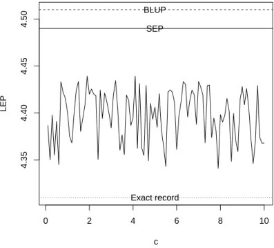
Figure 2 –Estimates of last record versuscof the Linex loss function.
the squared error loss function. We see that BLUP is the furthest from the exact record. The one based on the squared error loss function is the second furthest from the exact record. The predictions given by the asymmetric Linex loss are the closest to the exact record.
We also computed the 95 percent Bayesian prediction interval of the last record. It was(4.22, 4.56), containing the exact value.
6. SIMULATION AND DISCUSSION
In this section, different estimation and prediction methods are compared using a Monte Carlo simulation. We compare the performances of the MLEs, the BLUEs and Bayes point estimators (with respect to the squared error and Linex loss functions) in terms of biases, and mean squared errors (MSEs). We also compare two CIs, namely, the CIs based on BLUEs, asymptotic MLEs, bootstrapping and the HPD intervals based on the Monte Carlo method in terms of average confidence lengths, and coverage probabilities. For computing Bayes estimators and predictors, we assume two priors:
Prior 1: µ0=0, a=0, b=0, Prior 2: µ0=0, a=2, b=3.
Obviously, prior 2 is more informative than prior 1. The simulations were performed as follows:
1. simulatenupper record values from the standard normal distribution;
2. compute the MLEs, BLUEs and Bayes estimators based on the squared error and Linex loss functions. For the Linex loss function, we tookc=−1, 0.1, 1;
3. compute the 95 percent CIs based on BLUEs, asymptotic MLEs, bootstrapping and the 95 percent HPD intervals based on Monte Carlo simulations;
4. iterate over steps 1 to 3 ten thousand times.
This scheme gives for a givenn the biases and MSEs of the MLEs, BLUEs and Bayes estimators. It also gives for a givennthe average confidence lengths and coverage proba-bilities of the intervals based on BLUEs, asymptotic MLEs, bootstrapping and the HPD intervals based on Monte Carlo simulations.
Figure 3 plots the biases and MSEs of the estimators ofµandσversusn=5, 6, . . . , 10. Figure 4 plots the confidence lengths and coverage probabilities of the estimators ofµ andσversusn=5, 6, . . . , 10.
We can observe the following from Figure 3: the biases for the BLUE are the closest to zero as expected; the biases for the other estimators generally decrease to zero asn
zero asnincreases; the BLUEs have the largest MSEs, the MLEs have the second largest MSEs, the Bayes estimators based on the squared error loss have the third largest MSEs and the Bayes estimators based on the Linex loss have the smallest MSEs; the use of prior 2 leads to smaller biases and smaller MSEs.
5 6 7 8 9 10
0.0 0.1 0.2 0.3 0.4 n Bias
5 6 7 8 9 10
0.0
0.1
0.2
0.3
0.4
5 6 7 8 9 10
0.0
0.1
0.2
0.3
0.4
5 6 7 8 9 10
0.0
0.1
0.2
0.3
0.4
5 6 7 8 9 10
0.0
0.1
0.2
0.3
0.4
5 6 7 8 9 10
0.0 0.1 0.2 0.3 0.4 ML BLU BS, Prior 1 BL, Prior 1 BS, Prior 2 BL, Prior 2
5 6 7 8 9 10
0.0 0.1 0.2 0.3 0.4 n Bias
5 6 7 8 9 10
0.0
0.1
0.2
0.3
0.4
5 6 7 8 9 10
0.0
0.1
0.2
0.3
0.4
5 6 7 8 9 10
0.0
0.1
0.2
0.3
0.4
5 6 7 8 9 10
0.0
0.1
0.2
0.3
0.4
5 6 7 8 9 10
0.0 0.1 0.2 0.3 0.4 ML BLU BS, Prior 1 BL, Prior 1 BS, Prior 2 BL, Prior 2
5 6 7 8 9 10
0.0
0.5
1.0
1.5
2.0
5 6 7 8 9 10
0.0 0.5 1.0 1.5 2.0 n MSE
5 6 7 8 9 10
0.0
0.5
1.0
1.5
2.0
5 6 7 8 9 10
0.0
0.5
1.0
1.5
2.0
5 6 7 8 9 10
0.0
0.5
1.0
1.5
2.0
5 6 7 8 9 10
0.0 0.5 1.0 1.5 2.0 BLU ML BS, Prior 1 BL, Prior 1 BS, Prior 2 BL, Prior 2
5 6 7 8 9 10
0.0
0.5
1.0
1.5
5 6 7 8 9 10
0.0 0.5 1.0 1.5 n MSE
5 6 7 8 9 10
0.0
0.5
1.0
1.5
5 6 7 8 9 10
0.0
0.5
1.0
1.5
5 6 7 8 9 10
0.0
0.5
1.0
1.5
5 6 7 8 9 10
0.0
0.5
1.0
1.5 BLUML
BS, Prior 1 BL, Prior 1 BS, Prior 2 BL, Prior 2
Figure 3 –Biases and MSEs versusn: bias forµ(top left), bias forσ(top right), MSE forµ(bottom left) and MSE forσ(bottom right).
probabilities appear furthest from the nominal level for the BLUE CIs and closest to the nominal level for the HPD intervals based on prior 1 and prior 2.
5 6 7 8 9 10
1 2 3 4 n Length
5 6 7 8 9 10
1
2
3
4
5 6 7 8 9 10
1
2
3
4
5 6 7 8 9 10
1
2
3
4
5 6 7 8 9 10
1 2 3 4 BLUE MLE Bootstrap Prior 1 Prior 2
5 6 7 8 9 10
1 2 3 4 n Length
5 6 7 8 9 10
1
2
3
4
5 6 7 8 9 10
1
2
3
4
5 6 7 8 9 10
1
2
3
4
5 6 7 8 9 10
1 2 3 4 BLUE MLE Bootstrap Prior 1 Prior 2
5 6 7 8 9 10
0.948 0.950 0.952 0.954 0.956 0.958 n CP
5 6 7 8 9 10
0.948 0.950 0.952 0.954 0.956 0.958
5 6 7 8 9 10
0.948 0.950 0.952 0.954 0.956 0.958
5 6 7 8 9 10
0.948 0.950 0.952 0.954 0.956 0.958
5 6 7 8 9 10
0.948 0.950 0.952 0.954 0.956 0.958 BLUE MLE Bootstrap Prior 1 Prior 2
5 6 7 8 9 10
0.948 0.950 0.952 0.954 0.956 0.958 n CP
5 6 7 8 9 10
0.948 0.950 0.952 0.954 0.956 0.958
5 6 7 8 9 10
0.948 0.950 0.952 0.954 0.956 0.958
5 6 7 8 9 10
0.948 0.950 0.952 0.954 0.956 0.958
5 6 7 8 9 10
0.948 0.950 0.952 0.954 0.956 0.958 BLUE MLE Bootstrap Prior 1 Prior 2
Figure 4 –Confidence lengths and coverage probabilities versusn: coverage length forµ(top left), coverage length forσ(top right), coverage probability forµ(bottom left) and coverage probability forσ(bottom right).
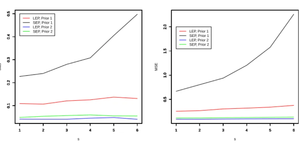
To see how the Bayes predictors based on priors 1 and 2 compare to each other, we also carried out a Monte Carlo simulation. We simulated a sample of ten upper record values from the standard normal distribution and used the first four to predict the sth record for s =5, 6, . . . , 10. We computed the Bayesian point estimators based on the squared error and Linex loss functions. We also computed 95 percent Bayesian PIs based on the squared error and Linex loss functions. The biases, MSEs, confidence lengths and coverage probabilities for every s were computed over ten thousand itera-tions as described before. Figure 5 plots the biases and MSEs of the predictors versus
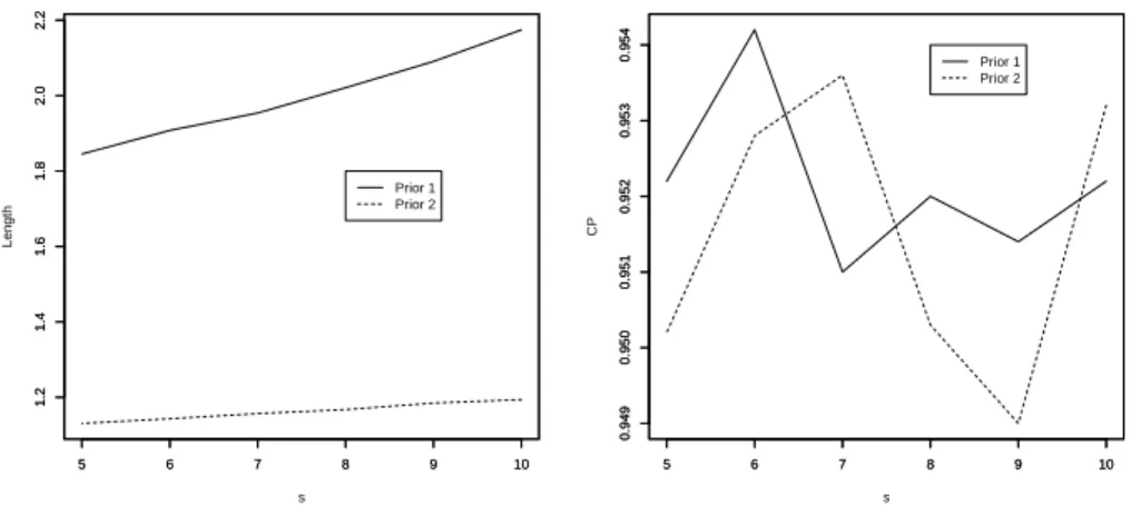
s =5, 6, . . . , 10. Figure 6 plots the confidence lengths and coverage probabilities of the Bayesian PIs versuss=5, 6, . . . , 10.
We can observe the following from Figure 5: the biases generally increase with in-creasings; the biases appear larger when the squared error loss is used and smaller when the Linex loss is used; the use of prior 2 leads to smaller biases; the MSEs generally in-crease with increasings; the MSEs appear larger when the squared error loss is used and smaller when the Linex loss is used; the use of prior 2 leads to smaller MSEs.
We can observe the following from Figure 6: confidence length generally increases with increasings; they appear larger for prior 1 and smaller for prior 2; coverage proba-bilities appear further from the nominal level for prior 1 and closer to the nominal level for prior 2.
1 2 3 4 5 6
0.1
0.2
0.3
0.4
0.5
s
Bias
1 2 3 4 5 6
0.1
0.2
0.3
0.4
0.5
1 2 3 4 5 6
0.1
0.2
0.3
0.4
0.5
1 2 3 4 5 6
0.1
0.2
0.3
0.4
0.5
LEP, Prior 1 SEP, Prior 1 LEP, Prior 2 SEP, Prior 2
1 2 3 4 5 6
0.5
1.0
1.5
2.0
s
MSE
1 2 3 4 5 6
0.5
1.0
1.5
2.0
1 2 3 4 5 6
0.5
1.0
1.5
2.0
1 2 3 4 5 6
0.5
1.0
1.5
2.0
LEP, Prior 1 SEP, Prior 1 LEP, Prior 2 SEP, Prior 2
5 6 7 8 9 10
1.2
1.4
1.6
1.8
2.0
2.2
s
Length
5 6 7 8 9 10
1.2
1.4
1.6
1.8
2.0
2.2
Prior 1 Prior 2
5 6 7 8 9 10
0.949
0.950
0.951
0.952
0.953
0.954
s
CP
5 6 7 8 9 10
0.949
0.950
0.951
0.952
0.953
0.954 Prior 1
Prior 2
Figure 6 –Coverage lengths and coverage probabilities versus s: coverage length (top left) and coverage probability (right).
Finally, we repeated the simulations for Figures 3 and 4 by contaminating the sim-ulated samples. Instead of simulating a sample of sizenfrom the standard normal dis-tribution, we simulated a sample of size(n−1)from the standard normal distribution and a sample size 1 from the Student’s tdistribution with one degree of freedom. We then computed the biases, MSEs, confidence lengths and coverage probabilities as be-fore. Plots of them versusnshowed a similar pattern to Figures 3 and 4: excluding the BLUEs, the MLEs had the largest biases, the Bayes estimators based on the squared error loss had the second largest biases and the Bayes estimators based on the Linex loss had the smallest biases; the BLUEs had the largest MSEs, the MLEs had the second largest MSEs, the Bayes estimators based on the squared error loss had the third largest MSEs and the Bayes estimators based on the Linex loss had the smallest MSEs; the use of prior 2 led to smaller biases and smaller MSEs; confidence lengths appeared largest for the BLUE CIs and smallest for the HPD intervals based on prior 2; coverage probabilities appeared fur-thest from the nominal level for the BLUE CIs and closest for the HPD intervals based on prior 2; and so on. But the magnitude of the biases, MSEs and confidence lengths were larger when compared to Figures 3 and 4. Also the coverage probabilities were further away from the nominal level when compared to Figure 4.
7. CONCLUSIONS
is observed that the Bayes estimators have clear advantages over the MLEs and BLUEs and that the Linex loss is superior to the squared error loss. We also used Monte Carlo simulations to compute Bayesian predictors of future records. Once again the Linex loss gave better predictions than the squared error loss.
ACKNOWLEDGEMENTS
The authors would like to thank the Editor and the referee for careful reading and for their comments which greatly improved the paper.
REFERENCES
J. AHMADI, M. DOOSTPARAST, A. PARSIAN (2005). Estimation and prediction in a
two-parameter exponential distribution based on k-record values under LINEX loss func-tion. Communications in Statistics-Theory and Methods, 34, pp. 795–805.
M. AHSANULLAH(1995).Record Statistics. Nova Science Publishers, Commack, New
York.
B. C. ARNOLD, N. BALAKRISHNAN, H. N. NAGARAJA(1998). Records. John Wiley and Sons, New York.
A. ASGHARZADEH, A. FALLAH(2011). Estimation and prediction for exponentiated
family of distributions based on records. Communications in Statistics-Theory and
Methods, 40, pp. 68–83.
A. ASGHARZADEH, R. VALIOLLAHI, D. KUNDU(2015).Prediction for future failures
in Weibull distribution under hybrid censoring. Journal of Statistical Computation and
Simulation, 85, pp. 824–838.
N. BALAKRISHNAN, P. S. CHAN(1998). On the normal record values and associated
inference. Statistics and Probability Letters, 39, pp. 73–80.
N. BALAKRISHNAN, A. C. COHEN(1991). Order Statistics and Inference: Estimation
Methods. Academic Press, San Diego.
A. P. BASU, N. EBRAHIMI(1991).Bayesian approach to life testing and reliability
estima-tion using a symmetric loss funcestima-tion. Journal of Statistical Planning and Inference, 29,
pp. 21–31.
M. CHACKO, M. MARY(2013).Estimation and prediction based on k-record values from
K. N. CHANDLER(1952).The distribution and frequency of record values. Journal of the
Royal Statistical Society: Series B, 14, pp. 220–228.
M. H. CHEN, Q. M. SHAO(1999).Monte Carlo estimation of Bayesian credible and HPD
intervals. Journal of Computational and Graphical Statistics, 8, pp. 69–92.
R. P. FEYNMAN(1987).Mr. Feynman goes to Washington. Engineering and Science, 51, no. 1, pp. 6–22.
D. KUNDU, H. HOWLADER (2010). Bayesian inference and prediction of the inverse
Weibull distribution for Type-II censored data. Computational Statistics and Data
Anal-ysis, 54, pp. 1547–1558.
D. KUNDU, B. PRADHAN(2009). Estimating the parameters of the generalized
exponen-tial distribution in presence of hybrid censoring. Communications in Statistics-Theory
and Methods, 38, pp. 2030–2041.
D. KUNDU, M. Z. RAQAB(2012).Bayesian inference and prediction of order statistics for
a Type-II censored Weibull distribution. Journal of Statistical Planning and Inference,
142, pp. 41–47.
V. B. NEVZOROV(2000).Records: Mathematical Theory. American Mathematical Soci-ety, Providence, Rhode Island.
R DEVELOPMENTCORETEAM(2016).R: A Language and Environment for Statistical
Computing. R Foundation for Statistical Computing, Vienna, Austria.
M. Z. RAQAB, J. AHMADI, M. DOOSTPARAST(2007). Statistical inference based on
record data from Pareto model. Statistics, 41, pp. 105–118.
M. Z. RAQAB, M. T. MADI(2002). Bayesian prediction of the total time on test using
doubly censored Rayleigh data. Journal of Statistical Computation and Simulation, 72,
pp. 781–789.
C. REN, D. SUN, D. K. DEY(2006).Bayesian and frequentist estimations and prediction
for exponential distributions. Journal of Statistical Planning and Inference, 13, pp.
2873–2897.
N. K. SAJEEVKUMAR, M. R. IRSHAD(2014). Estimation of the location parameter of
distributions with known coefficient of variation by record values. Statistica, 74, no. 3,
pp. 335–349.
A. A. SOLIMAN, F. M. AL-ABOUD(2008). Bayesian inference using record values from
Rayleigh model with application. European Journal of Operational Research, 185, pp.
H. R. VARRIAN(1975). A Bayesian approach to real estate assessment. In S. E. FEIN
-BERGE, A. ZELLNER(eds.),Studies in Bayesian Econometrics and Statistics in Honor
of Leonard J. Savage, North Holland, Amsterdam, pp. 195–208.
S. J. WU, D. H. CHEN, S. T. CHEN(2006). Bayesian inference for Rayleigh distribution
under progressive censored sample. Applied Stochastic Models in Business and Industry,
22, pp. 269–279.
A. ZELLNER(1986). Bayesian estimation and prediction using asymmetric loss function.
Journal of the American Statistical Association, 81, pp. 446–451.
SUMMARY
Based on record data, the estimation and prediction problems for normal distribution have been investigated by several authors in the frequentist set up. However, these problems have not been discussed in the literature in the Bayesian context. The aim of this paper is to consider a Bayesian analysis in the context of record data from a normal distribution. We obtain Bayes estimators based on squared error and linear-exponential (Linex) loss functions. It is observed that the Bayes estimators can not be obtained in closed forms. We propose using an importance sampling method to obtain Bayes estimators. Further, the importance sampling method is also used to compute Bayesian predictors of future records. Finally, a real data analysis is presented for illustrative pur-poses and Monte Carlo simulations are performed to compare the performances of the proposed methods. It is shown that Bayes estimators and predictors are superior than frequentist estimators and predictors.