Lam_unc_0153D_15497.pdf

(1)

INNOVATIVE METHODS FOR SOME STATISTICAL ISSUES IN

CLINICAL TRIALS

Diana Fong-Hor Lam

A dissertation submitted to the faculty at the University of North Carolina at Chapel Hill in partial fulfillment of the requirements for the degree of Doctor of Philosophy in the

Department of Biostatistics in the Gillings School of Global Public Health.

Chapel Hill 2015

(2)

(3)

ABSTRACT

Diana Fong-Hor Lam: Innovative Methods for Some Statistical Issues in Clinical Trials (Under the direction of Gary Koch)

Clinical trials have many different aspects to them, and here three topics will be explored: Bayesian sensitivity analysis in survival models, ROC methods in the presence of verification bias, and non-parametric adjustment of covariates in randomized clinical trial with and without missing data.

The aim of the first paper is to develop several Bayesian influence measures to assess the influence of the prior, the sampling distribution, and individual observations in survival analysis with the presence of missing covariate data and describe these changes in a modified likelihood model (the perturbation model). We construct a Bayesian perturbation manifold to the perturbation model and calculate its associated geometric quantities and influence measures based on several objective functions to quantify the degree of various perturbations to statistical models. We carry out several simulation studies and analyze a real data set to illustrate the finite sample performance of our Bayesian influence method.

While clinical trials concerned with survival track how long people will live given that they have the disease, some trials are concerned with using screeners to predict disease in the first place. Chronic obstructive pulmonary disease (COPD) affects 5% of the adult population in the United States, but a general screener has not been evaluated for the disease at a large scale. In this paper a COPD screener is evaluated using an innovative application of sampling weights. With these sampling weights, which help us adjust for verification bias, we explore the different variables to use in the screener. The optimal variable on the pocket screener was forced expiratory volume in 1 second as compared to peak expiratory flow.

(4)

(5)

(6)

ACKNOWLEDGEMENTS

(7)

LIST OF TABLES

2.1 FI for unperturbed and perturbed probability densities . . . 21

2.2 First order influence measures for E1684 data . . . 26

2.3 Observations with high75th percentiles . . . 28

2.4 Observations with high90th percentile values . . . 28

3.1 PEF Screener versus COPD status by office spirometry, un-weighted. . . 47

3.2 Calculation of weights . . . 47

3.3 Comparison of PEF between 3 groups of subjects . . . 48

3.4 PEF Screener versus COPD status by office spirometry, weighted . . . 48

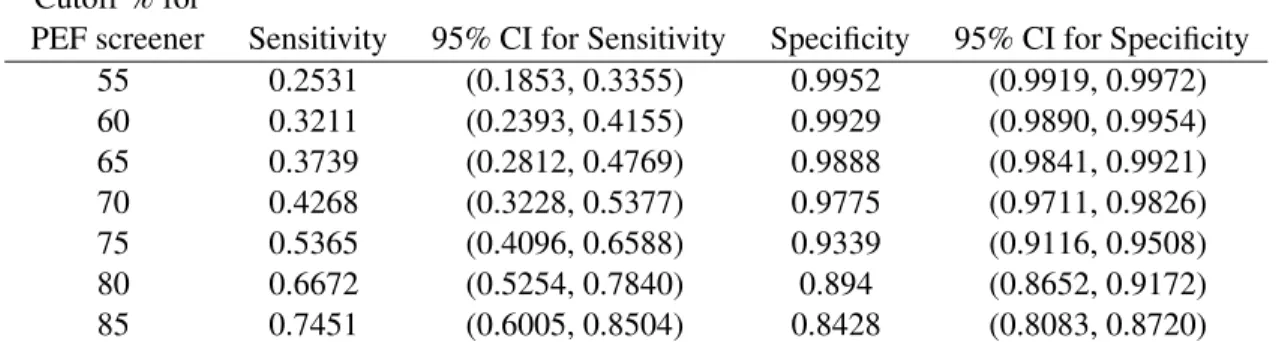
3.5 Sensitivity and specificity with 95% confidence interval (CI) for different cutoffs of PEF . . . 48

3.6 Unweighted values if cutoff of 91% had been used . . . 48

3.7 Weighted values if cutoff of 91% had been used . . . 48

4.1 Distribution of responses for Stokes et al. (2012) . . . 64

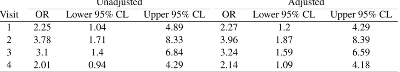
4.2 Comparison of OR for unadjusted and adjusted treatment effects by visit . . . 65

4.3 Comparison of overall treatment OR . . . 65

4.4 Table comparing treatment effects nested within visit for 2 methods . . . 68

4.5 Comparison of unadjusted and adjusted method for partial proportional odds model . . . 71

4.6 Comparison of unadjusted and adjusted OR with stratification by center . . . 77

4.7 Distribution of binary response pooled over treatment. . . 82

4.8 Distribution of binary response by visit and treatment . . . 82

4.9 Comparison of randomization based non-parametric covariate adjustment with unad-justed treatment estimates . . . 83

4.10 Lower95%CL of odds of responders on low and high dose at 3 time points . . . 86

4.11 Lower95%CL of proportion of responders on low and high dose at 3 time points . . . 86

4.12 Distribution of ordinal responses by treatment . . . 88

(12)

5.3 Number (percent) missing for covariates by treatment . . . 99

5.4 Estimates of the differences in means (treatment-placebo) of covariates from PROC GENMOD on original scale . . . 99

5.5 Summary of imputed data sets . . . 100

5.6 Full model results from Equation 5.8 on imputations of original data on original covariate scale . . . 101

5.7 Distribution of the missingness of size by treatment group . . . 103

5.8 Population based minimum and maximum for covariates (# in parenthesis is the un-logged value) . . . 103

5.9 Comparing estimates of three methods . . . 105

5.10 Summary ofbacross 100 bootstraps . . . 105

5.11 Summary ofVbacross 100 bootstraps . . . 108

6.1 Ranges used for transformation of covariates . . . 119

6.2 Imputed means for varaiables by disease onset site . . . 119

6.3 Distribution of missingness by treatment group . . . 120

6.4 Distribution of survival time (days) by treatment and censoring . . . 125

6.5 Distribution of covariates by treatment . . . 127

6.6 Distribution of mean of covariates by treatment group . . . 128

(13)

LIST OF FIGURES

2.1 First-order influence measure for Bayes factor . . . 30

2.2 First order influence measures for missing observations . . . 31

2.3 Graphic of FI measures across all 100 iterations . . . 31

2.4 Original FI values versus interquartile range (IQR) of 100 bootstraps . . . 32

2.5 Original FI values versus interdecial range (IDR) of 100 bootstraps . . . 33

3.1 ROC with confidece intervals around a variety of cutoffs . . . 49

3.2 Ratio (1−_specificitysensitivity) vs sensitivity . . . 53

3.3 ROC of PEF to they=xline and they=√xcurve . . . 54

3.4 Weighted ROC of PEF and FEV1 . . . 55

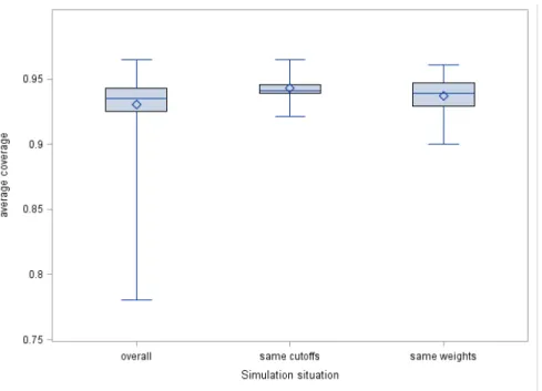
3.5 Summary of coverage of simulations exploring non-ignorable verification bias . . . 56

3.6 Graphic representation of components changed in the simulation . . . 56

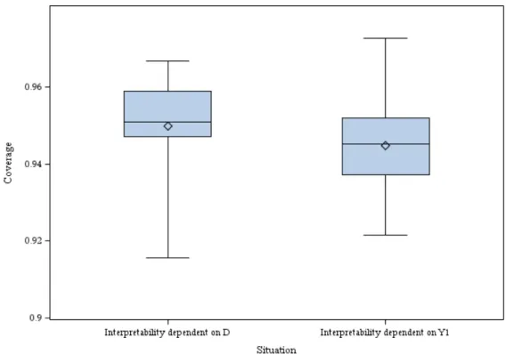
3.7 Summary of coverage of simulations exploring mismatch of study cutoff and disease interpretability cutoff . . . 57

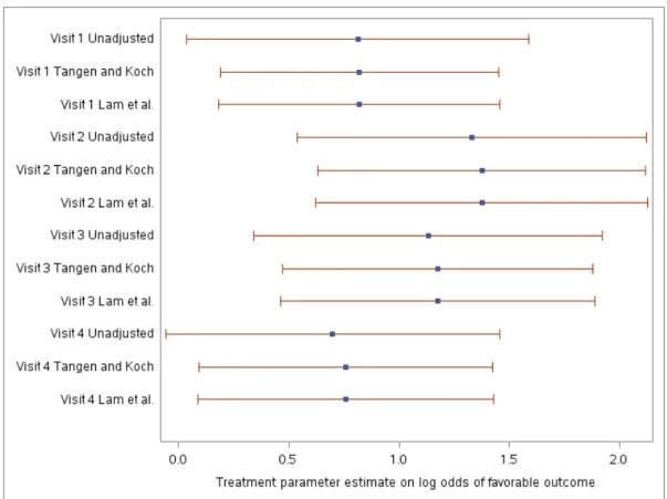
4.1 Forest plot comparing Tangen and Koch (1999) and current method . . . 67

5.1 Kaplan-Meier plot of treatment versus placebo . . . 98

5.2 Forest plot comparing three methods to handle missingness . . . 104

5.3 Boxplot ofbacross 100 bootstraps by method . . . 106

5.4 Boxplot of estimated standard error ofbacross 100 bootstraps by method . . . 107

5.5 Boxplot of p-values of covariates across 100 bootstraps . . . 108

5.6 Scatter plot comparing standard errors of multiple imputation method with dfbeta method over 100 bootstraps . . . 109

5.7 Scatter plot comparing treatment estimates of multiple imputation method with dfbeta method over 100 bootstraps . . . 110

6.1 Kaplan-Meier plot of 3 doses versus placebo . . . 124

(14)

CHAPTER 1: INTRODUCTION

In today’s world of clinical trials, there are many statistical analyses that we perform to adjust for the fact that trials occur in real life and are not carried out as perfectly as we would wish. There are methods to adjust for missing data, sensitivity analyses to test model assumptions, and weighting schemes to adjust the data to a more general population. Furthermore, clinical trials have many outcome variables that can be addressed: length of survival in the study, dichotomous outcomes such as diseased or non-diseased, or ordinal outcomes such as diseased, partially diseased, and non-diseased.

1.1 SURVIVAL ANALYSIS

In one type of clinical trial, the objective is to assess whether a treatment can improve the survival rates. There are many types of survival models. Survival models are inherently different from general linear models because they contain a censoring variable. Since it is unlikely that all patients in the study will experience the event or events during the time frame of the study, it is necessary to include a variable indicating whether or not the patient was event-free at the time they left the study or the time that the study ended.

A subject with an uncensored event is a subject who experienced the event of interest during the observed portion of the study. The event could be death, recurrence of disease, organ transplant, to name a few. A patient who is censored is a patient who does not experience the event during his time in the study. Patients may be censored for one of many reasons: they completed the study period without incident, they withdrew from the study, they were loss to follow-up, etc. For the purpose of this paper, it is assumed that all patients have a known starting time in the study. Therefore any censoring that occurs is right-sided censoring.

While many models use maximum likelihood methods by estimating parameters in the density function, survival models want to maximize survival, which is measured as a function of the cumulative distribution. LetF(t, β, x)be the cumulative distribution function for a subject at timet, and covariates in the vector

(15)

maximized must incorporate both the density of events and survivorship function. Therefore, a censorship indicator variable, C, is created, where C=1 if the subject experienced the event and C=0 otherwise.

The likelihood function we want to maximize for survival models for alli= 1, . . . , Nsubjects is N

Y i=1

[f(t, β, x)]c[S(t, β, x)]1−c

In order to estimate the survivorship function (S(t, β, x)), we use the cumulative hazard function and the density of the hazard function. The hazard function represents the risk of experiencing an event in an interval after time t, given that the subject has survived to timet(Hosmer and Lemeshow, 1999). If the hazard function can be estimated parametrically, it is usually modeled using traditional linear modeling methods. The cumulative hazard function is the sum of the hazards over all intervals.

If the hazard function has a parametric form, the hazard, cumulative hazard, and survivorship function are related with the following equations:

H(t) = Z t

0

h(u) du

S(t) = exp(−H(t))

A popular method for analyzing such data is the Cox proportional hazards model (Cox, 1972), which estimates the effects of the covariates on the hazard ratio with respect to an unspecified baseline hazard. It assumes that hazards are proportional between groups with respect to time. The model for the Cox proportional hazards model is

λ(t|zj) =λ0(t) exp(β0zj) (1.1)

whereλ0(t)is the baseline hazard given the subject had survived until timet,zj is the vector of covariate values for patientj, andβis the vector of treatment effect parameters.

1.2 MISSING DATA AND SENSITIVITY ANALYSIS

(16)

accommodate the censored structure of the data and account for binary, categorical, and continuous covariates. Ad hoc methods are sometimes used for treating missing data, such as carrying the last observation forward or imputing the missing value using the mean of the covariate (Little and Rubin, 1987). One of the earlier papers to address missing data in survival models was Schluchter and Jackson (1989). They specified the joint distribution of failure time and covariates as the conditional distribution of failure time given covariates, and a marginal distribution on covariates, which was treated as a nuisance parameter. Lin and Ying (1993) came up with an estimator using the approximate partial likelihood estimator. Zhou and Pepe (1995) expanded on this work and applied this EM-type algorithm to data that were missing at random and monotone.

Most methods assume that missing covariates are either missing completely at random (MCAR) or missing at random (MAR). Covariates that are MCAR means the missing data mechanism does not depend on the observed or missing observations (Little and Rubin, 1987). In other words the missing observations are themselves a simple random sample. Covariates that are MAR means the data missing mechanism depends on the observed values but not the missing values (Little and Rubin, 1987). The missing observations are a simple random sample given the observed values. Paik and Tsai (1997) proposes using multiple imputation to address the missing covariates under MAR conditions. Chen and Little (1999) introduce a non-parametric likelihood which uses a discretized version of the likelihood where the baseline hazard is cast as a step function with jumps at the observed values. This method requires the specification of the missing data distribution and assumes missingness is MAR. Furthermore the method is only valid for covariates that are all discrete or all normally distributed (Herring and Ibrahim, 2001). Another method of handling missing covariates is to use estimating equations to produce parameter estimates. These methods generally require the missing data mechanism to be specified. The likelihood often has an expectation of the complete data given the observed data. Lipsitz and Ibrahim (1998) have estimating equations that are applicable only to categorical covariates. Herring and Ibrahim (2001) expand on the methodology of Lipsitz and Ibrahim (1998) to the situation looking at both continuous and categorical covariates. They provide weighted estimating equations in the log likelihood where the weights are the probabilities of a particular missing data pattern for a subject. These methods (Lipsitz and Ibrahim, 1998; Chen and Little, 1999; Herring and Ibrahim, 2001) all use an EM algorithm (and possibly adaptive rejection metropolis sampling) to get estimates.

(17)

expanded on the methods of Leong et al. (2001), who had done work on non-ignorable data mechanisms for binary covariates, to the case when the non-ignorable mechanism was applied to both discrete and continuous covariates. More recently, Ibrahim et al. (2008) developed semi-conjugate priors for missing at random covariate data and developed a variation on DIC for survival models. As the methods become more complex, other papers such as Cho et al. (2009) have found creative ways of getting around computational issues for survival models.

Bayesian work in survival models has focused on two main areas: extending frequentist hypothesis testing methods into a Bayesian setting and developing more complex priors to better suit the nature of survival parameters. Sinha et al. (2003) extended Cox’s partial likelihood into a Bayesian context. Dunson and Herring (2003) developed Bayesian methods for testing null hypothesis versus order-restricted alternatives. In addition to exploring survival model testing, Dunson and Park (2008) developed a kernel stick breaking prior to model an uncountable number of random events. Other types of priors used in Bayesian survival analysis include beta process and Dirichlet process. The beta process treats discrete intervals of the hazard function as having a beta distribution. The Dirichlet process is a non-parametric prior that involves putting a Dirichlet distribution on the cumulative hazard over disjoint intervals. A more detailed summary of these priors can be found in Ibrahim et al. (2001).

Bayesian diagnostics on survival models and other generalized models has grown out of frequentist diagnostics. The most commonly used frequentist diagnostic is Cook’s distance (Cook, 1986). One extension of Cook’s distance is the conditional posterior ordinate (CPO), which can be thought of as the marginal posterior predictive density of theithcase if it were deleted from the data set (Gelfand et al., 1992; Gelfand, 1999; Wei and Su, 1999). In addition to case deletion diagnostics, there are also systemic and isolated departures to examine (Davison and Tsai, 1992). Systemic departures come about when features of the data set have not been captured or a large group of observations does not fit well. Isolated departures, such as outliers, arise when a few observations do not fit the model.

(18)

prior, and this method is called local sensitivity analysis. Although measuring the many different changes at once is possible, Gustafson and Wasserman (1995) suggested that examining individual elements of change is preferred. Hyperparameters or clusters that had high local sensitivity were a cause for concern. Zhu et al. (2007) developed advanced techniques for exploring clusters that did not fit well.

1.3 RECEIVER OPERATOR CHARACTERISTIC CURVES IN THE PRESENCE OF

VERIFICATION BIAS

Another aspect of clinical trials besides survival is determining whether continuous or categorical measures can be used to discriminate between diseased and non-diseased patients. Initially the methods developed were used to detect signals in the presence of noise(Green and Swets, 1966). Early evaluations focused on categorical measures. The estimates used to evaluate the measures were sensitivity, the probability of the test being positive given the subject was diseased, and specificity, the probability of the test being negative given the subject was not diseased. Eventually, methods were created to handle continuous measures. These methods created a Receiver Operating Characteristic curve (ROC curve), which plots the sensitivity versus 1-specificity at a variety of cutoff points, where the cutoff point differentiates between diseased and non-diseased subjects. The Area Under the Curve (AUC) gives a sense of the measures accuracy for differentiating between diseased and non-diseased states and ranges from 0.5 to 1. An AUC of 0.5 represents a measure whose accuracy is no better than a random guess, while an AUC of 1 represents a measure that predicts diseased or non-diseased status perfectly. The AUC corresponds to the Mann-Whitney statistic (Bamber, 1975).

In addition, statisticians can compare the AUC’s of multiple measures that were conducted on the same people to see if one measure is better able to discriminate than others (DeLong et al., 1988). Multiple tests or screeners can be tested on the same subjects in an effort to compare different screeners. The AUC’s for the different screeners are then correlated. Statistical tests that wish to determine whether one screener is significantly different than the other needs to take into account this correlation when calculating the variance of the difference between the AUC’s.

(19)

tests in the non-diseased group and the correlation between the two tests in the diseased group and the average of the AUC’s for each test was calculated. A derived table with average correlation along the rows and average area under the curve along the columns was then used to calculater. The standard error formula is the same as normal: SE(AUC1−AUC2) =

q

SE2(AUC1) +SE2(AUC2)−2×r×SE(AUC1)×SE(AUC2). In addition to calculating the correlation between the measures, it is also important to consider verification bias when calculating both the estimate of the difference between correlated AUC’s and the variance of the difference. There have been 2 main ways of dealing with verification bias: imputation and reweighting. Some of the imputation methods are full imputation (Rotnitzky et al., 2006; Alonzo and Pepe, 2005) and mean score imputation (Alonzo and Pepe, 2005). These imputation methods extend the ideas initially proposed by Begg and Greenes (1983) to screener tests with continuous outcomes. Unlike imputation methods that treat the disease status as missing, reweighting methods use only the subjects that has both test and disease information. But like imputation methods, reweighting methods assumes that the population of subjects with the test results is the population that we wish to make inference on.

For all methods described, letTibe the test result for theithperson,Vibe the indicator that theithpatient went on for disease verification,Dibe the true disease status, andXibe the vector of covariates of interest. Thus in the presence of verification bias, Ti, Vi,andXi are observed for all i= 1, . . . , npatients where

n=total number of patients in the study, andDiis missing for a subset of patients.

In the full imputation method the missing disease status is predicted by modelingP(D= 1|T, X). The disease status is replaced by the predicted probability of disease even for subjects whose disease status is known. The estimated probability of disease for theithpatient isρˆi=P(Di = 1|Ti, Xi). Therefore for the screener cutoff ofcthe senstivity with full imputation is

sens(c)FI=

Pn

i=1I(Ti ≥c) ˆρi Pn

i=1ρˆ

.

(20)

create an estimator for the disease status based on the model parameters, test result, and other measured covariates.

The model of log odds of no disease verification is expressed as

log

P r(V = 0|T, X, D)

P r(V = 1|T, X, D)

=h(T, X) +q(T, X)D. (1.2)

whereh(T, X)is a function of the test result and covariates associated with the log odds of not having disease verification depend on disease status that do not have any interaction with the disease status. Letq(T, X) be a function of how test result and covariates interact with disease status to influence the log odds of no disease verification. For example, if we had non-ignorable verification bias, then we expectq(T, X) 6= 0. Thenh(T, X)is assumed to have a parametric form such thath(T, X) =h(T, X|γ).

The next step is to model the probability of being diseased given that the subject went on for verification

log

P r(D= 1|V = 1, T, X)

P r(D= 0|V = 1, T, X)

=m(T, X). (1.3)

Letm(T, X)be a function of the test result and covariates that models log odds of disease status among those who have their disease status verified.m(T, X)is also assumed to have a parametric formm(T, X) =

m(T, X|µ).

The double robust estimator,DDR(γ, µ)i orDDRifor short, for theith patient’s disease status is

DDR(γ, µ)i =P(Vi, Ti, Xi|µ) +Ui(γ|µ)

where

Ui(γ, µ) =Vi[{Di−P(1, Ti, Xi|µ)}+ exp{h(Ti, Xi|γ)

(21)

and

P(Vi, Ti, Xi) =P r(Di= 1|Vi= 1, Ti, Xi)

× {Vi+

(1−Vi) exp{q(Ti, Xi)}

1−P r(Xi= 1|Vi= 1, Ti, Xi)× {1−exp{q(Ti, Xi)}}

}.

The process gives us 2 chances to get the model right. The estimator’s double robustness property means that if either the verification or disease model is mis-specified the estimator will still be consistent. DDRi is then calculated for all subjects and depends only on observed variables, therefore it can be calculated regardless of verification status. The estimator of the AUC is then calculated using the normal formula with

DDRisubstituted forDifor the entire data set. The formula for the AUC and its double robust estimator is

ν =P r(T2 > T1|D1= 1, D2= 0) + 0.5×P r(T2 > T1|D1 = 1, D2 = 0)

ˆ

ν = n P i=1

n P j=1

{DDRi(1−DDRj)×[I(Ti > Tj) +I(Ti =Tj)]}

n P i=1

n P j=1,j6=i

{DDRi(1−DDRj)}

.

Instead of treating the disease status as missing as in imputation methods, the inverse probability weighting (IPW) estimator uses weights to calculate the probability of verification. It weights each observation in the verified sample by the inverse of the probability of being selected for verification (Alonzo and Pepe, 2005). Letπˆi = P(Vi|Ti, Xi), which is estimated from disease-verified patients only. The estimate for sensitivity using IPW for the cutoffcis

sens(c)IPW=

Pn

i=1I(Ti ≥c){Vi∗Di/πˆi} Pn

i=1{Vi∗Di/πˆi}

.

This approach yields bias estimates of AUC when verification model is mis-specified (Alonzo and Pepe, 2005). However, in randomized studies, often the verification model is under investigators control. In these situations, investigators send a random sample of subjects on for verifiation based on pre-specified criteria.

(22)

sens(c)SPE=

Pn

i=1I(Ti≥c){Vi∗Di/ρˆ−(Vi−ˆπi)∗ρˆiπˆi} Pn

i=1{Vi∗Di/πî−(Vi−πî)∗ρî/πî}

.

This method is semiparametric since it parametrically modelsP(D|T, X)andP(V|T, X)but does not specify a distribution forP(D, T, X). This method is also doubly robust. Furthermore, this method combines both the efficiency of imputation methods with the robustness of re-weighting methods. Finally, another concern when evaluating ROC’s is the presence of verification bias, sometimes referred to as work up bias.

Selection bias, sometimes referred to as verification bias or work-up bias, occurs when the measures used to evaluate a test are based only on the subset of patients who had the disease verified (Begg, 1987). The stronger the association between the test result and disease verification, the larger the bias (Begg, 1987). The bias is important to adjust for since positive tests will be over-represented in the disease-verified population, leading to artificially inflated sensitivity and deflated specificity estimates.

Another bias that occurs is the bias of uninterpretable results. Uninterpretable results are those that are

technicallyunacceptable. For example, if the test is an ultrasound of the pancreas and the pancreas cannot be viewed, the test is uninterpretable (Begg et al., 1986). This is different from indeterminate results in which the meaning of the test is unclear. In situations in which the test result is uninterpretable, the uninterpretable subjects may be biasing the results if the uninterpretability is associated with test results (Begg et al., 1986). Begg et al. (1986) suggests adjusting the posterior odds by the probability of the odds of uninterpretable results of diseased groups to non diseased groups. Another suggestion by Begg et al. (1986) was to consider the uninterpretable readings as non-diseased, and adjust the numerator and denominator of specificity by that number.

1.4 NON-PARAMETRIC COVARIATE ADJUSTMENT IN LONGITUDINAL BINARY AND

ORDINAL SETTINGS

(23)

meaning that covariate imbalances between the treatment group(s) and control(s) are due to random chance. Non-parametric adjustment of covariates exploits this assumption of random covariate imbalance.

The advantages and limits of covariate modeling versus non parametric modeling have been outlined extensively by Tangen and Koch (1999). Some of the advantages of traditional covariate modeling are that the odds ratio for the treatment applies to patients in the same subpopulation according to the covariates in the model (Tangen and Koch, 1999). That then assumes that the patients at each cross classification of the covariates represent a stratified simple random sample of subjects based on explanatory variables. Also, traditional methods produce estimates of the effect of the covariates. Furthermore, non-parametric adjustment treats covariates and stratification variables differently while modeling treats them the same (Tangen and Koch, 1999). The main advantage of non-parametric adjustment is that it generally reduces the variance of the treatment effect without impacting the parameter estimate itself, and the treatment effect is still applicable to the general population the subjects come from (Koch et al., 1998). One of the advantages of adjusting non-parametrically is that the sample size only needs to take into account the number of parameters that pertain to treatment, without regard for the number of covariates you wish to adjust by.

After adjusting for covariates, we still have multiple ways of modeling the treatment effect, depending on the outcome variable. Oftentimes, the outcome variable in clinical settings is a dichotomous variable, however, there has been some work to extend methodology to an ordinal outcome. A few different methods deal with ordinal outcome variables. The generalized logistic regression model developed by McCullagh (1980) models the log of the probability of one level with respect to the probability of a reference level of the outcome variable. For simplicity’s sake, we will assume the reference level isj = 1, although in reality, the reference could be any level ofY. LetYi be the outcome for theithsubject, whereYi ∈1, . . . , k,

γj =P r(Y =j|x), andxibe a vector of covariates for theithsubject. The generalized logistic regression models

log

γj

γ1

=αj+x0βj, j = 2, . . . , k,

whereαjrepresents thejthlog odds ratio of thejthoutcome to the first outcome, holding all other variables constant.β_jrepresents the effect of the covariates on the log odds ratio of thejth_{outcome with respect to the}

(24)

Unfortunately, the generalized logistic regression has two disadvantages when the outcome is ordinal. As each outcome level except the reference has its own parameter effects and intercept, the sample size required to produce stable parameter estimates is large. It does not make use of the ordinal nature of the outcome variable, as odds are calculated with respect to a reference level. A model that does make use of the ordinal nature of the outcome variable is the proportional odds model developed by McCullagh (1980). Let

πj =P r(Y ≤j|x), so the linear model is

logit(πj) =αj+x0β, j= 2, . . . , k.

In this setting,αj represents the log odds ratio ofY ≤ jif all covariates are equal to 0. βrepresents the effect of the covariates on the log odds of more favorable values to less favorable values. This model requires that the effect of the covariates be the same regardless of which value differentiates between a success and failure for the odds, as there is only one parameter of covariate effect regardless of theπj being modeled. This assumption is called the proportional odds assumption and requires the data to check.

A model that combines features of the 2 is the partial proportional odds model, developed by Peterson and Harrell (1990). It can be modeled as

logit(πj) =αj+x0β+tφj

wheretis a vector of a subset of the original covariates which do not satisfy the proportional odds assumption. The partial proportional odds model uses both the ordinal nature of the outcome, and relaxes the proportional odds assumption for the covariates in the model. The advantage of this model is that for covariates for which proportional odds holds, we only need one parameter (expressed inβ, but we still have flexibility for covariates which do not satisfy the proportional odds assumption.

(25)

mixed model (GLMM) method the correlation is treated like an additional parameter to be estimated. The GLMM method requires large sample sizes, so if the correlation of the outcome variable between repeated visits is not of interest to inference, then the GLM method is more practical to use.

Within the GLM method, there are 2 methods for adjusting for the correlation between repeated measures. Maximum likelihood methods require specifying the correlation structure between measurements. However this can lead to bias if the correlation structure is mis-specified. An alternative method for parameter covariance estimation is to use generalized estimating equations (Liang and Zeger, 1986). The advantage of this method is that it is robust even if the correlation structure is mis-specified. Generalized estimating equations use a generalized linear model to estimate the marginal distribution of the outcome variable, and then uses a combination of sandwhich estimators and working correlation matrices to estimate the parameter and its covariance (Liang and Zeger, 1986).

Zeger et al. (1985) formed a model for the analysis of binary longitudinal data with time-independent covariates. If we letYitbe the binary outcome variable for theithsubject for thetthtime point andXibe the covariate vector for theith subject, then Zeger et al. (1985) modelsπi =P r(Yit= 1)and the correlation between consecutive time pointsρ. The models used islogitπi=X0iβwhereβis the effect of the covariates on the log odds ratio andcorr(Yit, Yi,t−1) = ρ. This model treats the binary series as the realization of a stationary Markov chain. One of the issues with this method was that there might also be correlation between outcomes that were more than 1 repeated measure apart. Furthermore, all time dependence is modeled in one parameter:ρ.

Stram et al. (1988) formed a more flexible model than Zeger et al. (1985) that could also work for repeated ordered categorical outcomes. The model relies on the proportional odds assumption for marginal probabilities, and each time point has its own model. By modeling each time point separately, the dependence between time points does not need to be modeled and instead is calculated empirically. Furthermore, the paper suggests a multi-stage testing procedure to check whether the time coefficients are significantly different from each other. The procedure relies on the fact that all hypotheses need to be rejected to move on to a subset of the hypothesis.

(26)

the null hypothesis p = 0.5. The estimate of p,pˆis then adjusted by Pd

c=1γˆc(ˆqc−0.5)where qˆc is

P r(Qc0 < Qc1) + 0.5P(Qc0 =Qc1). Qciis the value of thecthcovariate for theith treatment group. γˆc is then estimated from the covariance matrix of the covariates with each other and the covariates with the outcome. This method is similar to a simplified version of the method we propose. The advantages of our method is that we calculate the estimate of the difference between the two groups and the calculation ofˆγis unnecessary.

(27)

CHAPTER 2: BAYESIAN SENSITIVITY ANALYSIS IN SURVIVAL MODELS

2.1 INTRODUCTION OF SURVIVAL DATA SET IN ONCOLOGY STUDY

In this paper, we extend the methods of Zhu et al. (2007, 2010) to data from the Eastern Cooperative Oncology Group (ECOG), who carried out a phase III clinical trial for high dose interferon on multiple melanoma patients. In this data set, we haven = 285subjects and either their time to relapse or time to censoring. There were 196 relapses and 89 censored observations. The four covariates of interest are treatment, age, Breslow score, and size. Breslow score and size had missing values.

Briefly, Zhu et al. (2007) outlines 4 steps to calculating Bayesian local sensitivity measures for survival models.

1. Define what aspects of the model are to be tested, ie, individual data points, prior assumptions, etc, and create a vector,ωthat is associated with these aspects

2. Adjust the likelihood model such thatωis incorporated

3. Choose how sensitivity will be measured (posterior mean distance,φ-divergence,. . .)

4. Calculate sensitivity measures that are generally derivatives of the adjusted likelihood in step 2 with respect toω

We will apply this method to both a simulation, a real data set, and then we will explore some of its properties using a bootstrap simulation.

(28)

This chapter is organized as follows, in Section 2.2, we develop measures for calculating first and second order influence measures. Since the measures are based on geometric tensors and covariant derivatives as described in differential geometry and require only a proper sampling distribution, the censoring in survival models does not pose a problem. In Section 2.3, we apply the influence measures to a variety of simulated data sets and the ECOG data. In Section 2.4, explore the properties of the Bayesian influence measures via bootstrap samples of the ECOG data set. Section 2.5 contains a discussion of the measures.

2.2 BAYESIAN SURVIVAL MODELS WITH MISSING COVARIATES

2.2.1 STATISTICAL SURVIVAL MODELS WITH MISSING DATA

When covariates are missing, we need to think about whether or not the data are missing completely at random (MCAR), missing at random (MAR), or missing not at random (MNAR). To access aspects of the missingness pattern, we need to first establish some notation. For our data, we letDo = (x1,o, ..., xn,o),

Dm= (x1,m, ..., xn,m), andDc= (Do, Dm)represent the observed, missing, and complete data respectively. Letxi,mbe the vector of missing values for theithsubject andxi,obe the vector of observed values. The vector of covariates for theith subject isxi = (xi,m, xi,o) fori = 1, . . . , n. For missing data problems, we want to modelp(Dc|θ)as the product ofp(Do|θ)and a model of the missing data given the observed data (p(Dm|Do, θ)), whereθis a vector of necessary parameters. We usually use Markov chain Monte Carlo (MCMC) methods to simulatep(θ|Do)∝

R

p(Dc|θ)∗p(θ)dDm. With missing data, we also need a

missingness indicator,rij, to indicate missingness of thejthcovariate of theithsubject. Therefore,rij = 1 ifxij is missing and0otherwise, and each subject’s missingness vector isri. Whilei= 1, . . . , nand the number of covariates isp,jgoes from1, . . . , qwhere q is the number of possible missing covariates,q≤p, and the difference (p−q) is the number of completely observed covariates. Finally, letyi represent the survival data for theithobservation, with covariatesxi fori= 1, . . . , n.

(29)

response, then a complete case analysis will lead to unbiased results. In both the MCAR and MAR case, the data missing mechanism can be ignored. When the data are MNAR then the probability of observing

xi conditional on the observed data is dependent on the missing data itself. Again, if missingness does not depend on the response, a complete case analysis will be unbiased (Ibrahim et al., 2005).

We can model the probability of theithobservation having a particular survival time, covariate values, and missingness indicator as

p(yi, xi, ri|θ) =p(yi|xi, θ)∗p(xi|θ)∗p(ri|xi, yi, θ)

p(yi|xi, θ)is a general survival model, which depends on the covariates being known.p(x1|θ)is a model for the covariates, both missing and observed, andp(ri|xi, yi, θ)is the model of the missingness indicator of the covariates. One way to perturb the missing data mechanism from MAR to MNAR is to use a Bayesian Perturbation Maniforld.

2.2.2 BAYESIAN PERTURBATION MANIFOLD

The mechanics of measuring perturbations has its roots in differential geometry. We first choose a function that we would like to evaluate our diagnostic measures with respect to; measures such as the Bayes factor,

φ-divergence, Kullback-Leibler distance (KL distance) to name a few. Then, we envision the function as a manifold, or surface in more than 3 dimensions, over all changes of interest. The change in the manifold curvature going in one direction of change represents the amount of change that perturbation affects. There are certain guidelines as to what makes a viable perturbation scheme.

We represent pertubations to the complete-data model,p(Dc, θ)using the vectorω=ω(Dc, θ)in a set Ω. For example, if we are interested in investigating if our model has heteroscedastic variance in a general

linear modelYi=xiβ+i, i ∼N(0, σ2)and we wish to use the Bayes factor to measure how the pertrubed model changed from the unperturbed model, we would go from our unpertubed model,Yi ∼N x0iβ, σ2

to the pertrubed modelYi|ω ∼N

x0_iβ,σ_ω2

i

(30)

follow the rules of probability. For example, if we perturb the sample variance, thenR

p(y|ω)dy = 1and

p(y|ω)>0. Ideally each element ofωneeds to be independent, and the vector elements need to be scaled so that the effect sizes are comparable. For example, when using Cook’s distance to examine clustered data, larger clusters have more influence due to their size (Zhu et al., 2007). Perturbations should not have this problem.

We put the perturbations in a geometric framework called a Bayesian perturbation manifold. We can consider all possible perturbations of interest as a Riemannian Hilbert manifold under some conditions,

M =p(Dc, θ) :ω ∈Ω. We can parameterize tangent curves fromωas

C(t) =p(Dc, θ|ω(t)) : [−, ]→M, C(0) =p(Dc, θ|ω)

and R _˙

l(Dc, θ|ω(t))2p(Dc, θ|ω(t))dDcdθ <∞. OnM we define the tangent space of all possible curvesM at

ωas those curves that take form ofC(t)asTωM. We can define the inner product of two tangent vectors

v1(ω)andv2(ω)onTωM as

< v1, v2 >(ω) = Z

{v1(ω)v2(ω)}p(Dc, θ|ω)dDcdθ (2.1)

In TωM we can measure pertrubations. We look at several measusres: G(ω0),FIRI[v](ω(0)) and SIRI[v](ω(0)). These terms approximately represent distance, first-order curvature of the manifold, and second-order curvature of the manifold. The geometric tensor,G(ω)is defined as

G(ω(0)) = Z

[∂ωl(Dc, θ|ω(0))]⊗2p(Dc, θ|ω)dDcdθ (2.2)

. If the covariant derivative,∇_vu(ω)6= 0then we use first-order influence measure (FIRI[v](ω(0))) as the diagnostic of interest. If∇_vu(ω) = 0then use we use the second-order influence measure (SIRI[v](ω(0))) as the diagnostic. The covariant derivative∇_vu(ω)measures the initial rate of change ofIF(ω0)as we move fromω0in the direction ofωand is defined as∇vu(ω),

du[v](ω)−0.5{u(ω)v(ω)p(zcom,θ|ω)− Z

(31)

The first and second order influence measure are written with respect to an intrinsic influence measure, IF(ω) =IF(p(θ|zobs,ω)). We are usually interested in lettingIF(ω)representφ-divergence, the Bayes Factor, or the posterior mean.

We must then define a relative intrinsic influence measure (RIFM, RI(ω, ω0)) as a function of both

p(θ|Do, ω)andp(θ|Do, ω0)so that the difference in the intrinsic influence measure between the perturbed and unperturbed situation can be measured on the Bayesian Perturbation Manifold. The simplest example is to letRI(ω, ω0) =IF(ω)−IF(ω0). In addition, we want to scale theRI(ω, ω0)by the minimal geodesic distance betweenp(Dc, θ|ω)andp(Dc, θ|ω0). We will define this as the intrinsic influence measure.

IGIRI(ω,ω0) = RI(ω,ω0) 2

g(ω,ω0)2 . (2.4)

Since we are in the spaceT ωM, we can describe the local behavior ofRI(ω, ω0)asRI(ω(t), ω0)as

t→0along all possible curvesp(Dc, θ|ω(t))passing throughω(0) =ω0. The first-order influence measure is defined as

FIRI[v](ω(0)) = lim

t→0IGIRI(ω(0),ω(t)) =

{d(RI)[v](ω(0))}2

<v,v>(ω(0)) (2.5)

When ∂RI(ω(0)) = 0, the first-order influence measure is 0, so we use ∂2RI(ω(0)) to calculate the second-order influence measure, defined as

SIRI[v](ω(0)) = ∂

2_RI(_ω₍₀₎₎

<v,v>(ω(0)) (2.6)

We can structure the missing data as a sequence of one-dimensional conditional distributions as in (Ibrahim and Lipsitz, 1999). In order to deal with missing data, we cast the influence measures,F IRI(v) orSIRI(v)as an expectation with respect to the joint distribution of the parameters and missing data. We use Gibbs sampling in adaptive rejection Metropolis sampling (ARMS) to get an empirical missing data distribution. We treat the missing values for each observation as a parameter to be estimated in Gibbs sampling, meaning that each observation that was missing was modeled with a prior distribution. The parameters for the missing variable distribution can be thought of as nuisance parameters.

(32)

rejection metropolis sampling to get an empirical missing data distribution. We treat the missing values for each observations as a parameter to be estimated in Gibbs sampling meaning that each observation htat was missing was modeled with a prior distribution.

When we want to perturb the missing data mechanism from MAR to MNAR, then we perturbp(ri|yi, xi, θ), where xi = (xi,o, xi,m). Therefore the missingness will depend on both the observed (xi,o) and unob-served (xi,m) covariates. Sinceri is a binary variable vector, we perform a logistic regression onriwith the observed covariates and failure time as the predictors. To model the missingness indicator, we have

logit[P(ri = 1|ω)] =φ0+φ1yi+ωxi, whereφ0is the intercept,φ1is the coefficent of the failure time, and

ωis a perturbation of the affect of the observed covariate. Letφ0 andφ1be hyperparameters, used in the following logistic regression:

P(ri= 1|xi, yi) = (2.7)

exp{φ0+φ1yi+ωxi} 1 + exp{φ0+φ1yi+ωxi+}

ri

1

1 + exp{φ0+φ1yi+ωxi} 1−ri

.

When we have more than one covariate missing, we can use the following one-dimensional conditional distribution of the missing variables to simplify the distrubtion of the missing covariate:

logit[P(riq = 1|ri1, . . . , riq−1, xi,o, yi)] =φ0+φ1yi+ ˜ωq0x˜iq+φ0xi,o (2.8)

logit[P(riq−1 = 1|ri1, . . . , riq−2, xi,o, yi)] =η0+η1yi+ ˜ω0q−1x˜iq−1+η0xi,o ..

. (2.9)

logit[P(ri1 = 1|xi,o, yi)] =ψ0+ψ1yi+ω1xi1+ψ0xi,o.

(33)

2.3 EXAMPLES

2.3.1 SIMULATEDWEIBULL

We performed a simulation study for the Weibull model to determine whether our method was accurately detecting perturbations. We wanted the final data set to haven= 250observations. The failure times were chosen from

Yi|xi ∼W eibull(α,exp(˜x0iβ)) (2.10)

fori = 1, . . . , n. The vectorx˜i = (1, xi)wherexi is a simulated continuous covariate distributedXi ∼

N(0,1). βis the parameter of the effect of the intercept and covariateβ = (β0, β1)0. Letαaffect the rate of the hazard, andθ= (β0, α)0. Censoring times were created from an Exponential(0.5) distribution. The observed time was the minimum of the failure and censoring time. Overall 32% of the observations were censored.

Next, we added missingness to the covariates. We let the covariate be missing at random. The probability of missing depended on a random Bernoulli(logit−1(1.5 + 0.2∗yi)) variable, where the probability of missing depended on failure time. Overall we had 21.2% missing covariates.

In addition to creating the data set, we needed to have 5 observations for the influence measure to detect. We let the first 245 failure times come from the unperturbed Weibull distribution (2.10), but observations 246-250 came from a perturbed model. Instead of the normal hazard:h(t|xi) =αt(α−1)exp(β0+β1xi), we perturb the hazard for the last 5 observations toh(t|xi) =αt(α−1)exp(β0+β1∗xi−2x2i). The difference of2xican be represented in the perturbed hazard as:

h(t|xi, ωi) =αt(α−1)exp((β0+β1xi)−ωi), ω(0) = (0, . . . ,0). (2.11)

The perturbation to the hazard implies we have also pertrubed the log-likelihood:

l(p(y|α, β, ω)) =dlog(α) + n X

i=1

[vi(α−1) logyi+vix˜0iβ+viω−yαi exp(˜x0iβ+ωi)] (2.12)

(34)

Having simulated the data, we also needed to come up with priors forβ andα. We chose flat priors for both parameters,β∼N2 (0,0)0,10−6I2

whereI2is a2×2identity matrix, andα∼Γ(0.001,0.001). The true values areβ= (0.5,−1)0,andα= 2. The prior on the missing covariates was a normal distribution with the mean and variation of the observed covariates.

The geometric tensor for our perturbation to the prior is the n×n identity matrix. Therefore, the perturbation does not need to be shifted or scaled. The first-order influence measure for the Bayes factor for theith_{observation is}

F IRI[vi](ω(0)) =

I(vi= 1)− Z

y_iαexp(˜x0_iβ+ωi)p(β, α|Do)dΛ(α, β) 2

. (2.13)

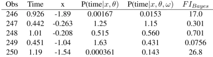
Table 2.1: FI for unperturbed and perturbed probability densities Obs Time x P(time|x, θ) P(time|x, θ, ω) F IBayes

246 0.926 -1.89 0.00167 0.0153 17.0

247 0.442 -0.263 1.25 1.15 0.301

248 1.01 -0.208 0.515 0.560 0.701

249 0.451 -1.04 1.63 0.431 0.0756

250 1.19 -1.54 0.000361 0.143 26.8

As Table (2.1) shows, there are two points that have a large FI. Given our perturbation scheme, we suspect that these two points may have a different hazard function that the rest of the data, as the Bayes factor has a large change for observations 246 and 250. As we can see from Table 2.1, observations 247-249 have very small influence measures. Since we know the hazard function that generated these points, we can look at the presumed probability density (p(time|x, θ)), and the true probability density (p(time|x, θ, ω)). For the observations with high FI values, we see that the observations are much more likely under the perturbed density than the unperturbed density. For the observations with small FI values, it can be seen that the observations do not have a large difference in densities.

(35)

2.3.2 PIECEWISE EXPONENTIAL

We applied the piecewise exponential model to data from the Eastern Cooperative Oncology Group, who carried out a phase III clinical trial for high dose interferon on multiple melanoma patients. Survival time was defined as the time between enrollment in the study and progression of the tumor or death, whichever came first. In this data set, we haven= 285subjects and either their time to relapse or time to censoring. There were 196 relapses and 89 censored observations. The 4 covariates of interest are treatment (binary), age (17-78 years), Breslow score (0.2-35), and size (0-476). Only the Breslow score which measures the thickness of the tumor and size (area) of the tumor have missing observations (30 and 55 respectively, and 11 with both covariates missing). Breslow and size were log transformed in order to use a normal distribution, and their log values were standardized. Observations with a fail-time of 0 were recorded as 0.01 since survival times are always positive.

The piecewise exponential model is constructed by partitioning the time axis at times0< s1 < s2 <

. . . < sJ, wheresJ is large enough to ensure that no survival times fall outside of it. Within each of the J intervals[0, s1),[s1, s2), . . . ,[sJ−1, sJ)we assume a constant hazard, i.e. an exponential survival function for the interval. We also chose to model three windows. They went from [0,0.378), [0.378, 1.16), [1.16, 10). There were approximately equal number of failures in each window.

The hazard for theith subject with covariatesxi over thejth time interval ish(t) = exp(φj +x0iβ) forsj−1 ≤t < sj. For the complete data distribution, we have two parameters of interest: β, andφ. Let

β represent the effect of the covariates of interest, which we assume remains the same for all windows andφa vector of the log of baseline hazards for theJ time windows. As the range for both parameters is (−∞,∞), we use multivariate normal (MVN) priors on both. We modelβ∼M V N4(µ0,Σ0)whereΣ0is a large multiple of the 4x4 identity matrix. Letφbe modeled asφ∼M V NJ=3(γ0, diag(a1, a2, a3)), where

diag(a1, a2, a3)is a diagonal matrix whose diagonal is formed by the enclosed vector.

In addition to the complete data distribution, we also need to define the missing variable distribution. This data set has two possible missing covariates. We divide the missing observations into 3 groups: (1) those with only Breslow score missing, (2) only size missing, and (3) both missing. We express the vector of missingness for theith observation asxi,m. When the ith observation is missing only Breslow score,

xi,m ∼N(η1, σ11). When theithobservation is missing only the size,xi,m ∼N(η2, σ22). When theith observation is missing both covariates,x ∼ M V N (η= (η , η )0,Σ), whereΣ = σ112 σ12

(36)

and variance of the observation missing only Breslow or only size is the respective marginal distribution of the observation missing both covariates. We can express all three situations asxi,m ∼M V Ndi(ηei,Σsi),

where in the case of only Breslow score missing,di = 1, ηei = η1,Σsi = σ11. In the case of only size

missing,di= 1, ηei =η2,Σsi =σ22. In the case of both covariates missing,di = 2, ηei =η,Σsi = Σ.

The missing variable distribution has two parameters of interest:ηandΣ.ηis a 2-dimensional vector of the mean of the missing Breslow scores and sizes whileΣis the covariance matrix of the bivariate distribution. We letη ∼M V N2(ζ0,Ψ0) and modelΣ ∼ W ishart2(c0, d0 ∗I2), wherec0 andd0 are scalars, andI2 is the 2-dimensional identity matrix, asΣis a semi-positive definite matrix. All multivariate normal prior distributions have means of 0 and variances of106. We letc0 = 2andd0 = 0.5which corresponds to an uninformative prior for the Wishart distribution.

The priors for the parameters may not reflect the true situation. If we have previous data on the covariates of interest, we may be interested in modeling a less flat prior onβ. The prior onφassumes that the baseline hazards are independent for each interval. We may also be interested in allowing the mean for each missing observation to vary, so that instead of all the missing breslow and size covariates having the same mean, they would depend on which observation was missing. These changes to our model can be represented as perturbations.

When performing model diagnostics, it is important to assess whether the model is sensitive to these perturbations. We could explore how reducing the variance would effect the model by perturbing the variance terms ofβ. Our perturbed prior would be

β|ω∼N4

µ0, diag(

σ2 1

ωβ1

, σ

2 2

ωβ2

, σ

2 3

ωβ3

, σ

2 4

ωβ4 )

. (2.14)

If we want to explore whether or not the baseline hazards are independent, we can perturb or change the prior onφ. We perturbφsuch that

φ|ω ∼M V N3(γ0, AR(ω)), AR(ω) =      

a1 ωφ1 0

ωφ1 a2 ωφ2

0 ωφ2 a3      

. (2.15)

(37)

If we were interested in modeling a separate mean for each missing observation, we could change the missing variable distribution forxi,m. Instead ofxi,m∼M V Ndi(ηei,Σsi)we can explore,

xi,m|ωimis ∼M V Ndi ωimis1

0

di +ηei,Σsi

(2.16)

whereωimishas the same dimension asxi,m. Written out for each of the three scenarios, we have

xi,m|ωimis∼N(ωimis+η1, σ11) if only Breslow missing (2.17)

xi,m|ωimis∼N(ωimis+η2, σ22) if only size missing (2.18)

xi,m|ωimis∼M V N2 (ωimis1, ωimis2)∗(1,1)0+η,Σ

if both missing. (2.19)

Letωimis = (ωimis,1, ωimis,2) ifxi is missing 2 variables and ωimisis scalar if xi is missing only 1 variable. As we have 72 observations with one or two covariates missing, and 83 values of either Breslow score or size missing. Therefore,ωmisis a vector with 83 elements, one for each missing value. All together,

ω= (ωβ, ωφ, ωmis)whereωβ corresponds to the scaling perturbations onβ,ωφto covariance between the log baseline hazards (φ), andωmisto the missing means ofxi,mandω0= (1,1,1,1,0,0,0, . . . ,0)89×1.

Using these perturbations, we calculate the complete log posterior to be

(2.20)

which we will use to calculateG(ω)andF IRI[v].

The geometric tensor is a block diagonal matrix composed of three block matrices along the diagonal. The first block matrix in the diagonal corresponds toG(ωβ)4×4 =diag(1₂,1₂,1₂,1₂). The second block matrix

corresponds toG(ωφ)2×2=   

1 a1a2 0

0 _a1

2a3

  +Eω

  

φ22

a1a22

+ φ21

a2 1a2

φ1φ3

a1a2a3

φ1φ3

a1a2a3

φ2 2

a2 2a3 +

φ2 3

a2a23

 

, whereaiis thei

th_diagonal

(38)

element ofg(Σ)is

gi(Σ) =                                Eω 1 σ11

if theithmissing observation only has the Breslow score missing

Eω

1 σ22

if theith_{missing observation only has the size missing}

Eω σ22 det(Σ) + σ11 det(Σ)− 2σ12 det(Σ)

if theithmissing observation has both missing

(2.21)

Since bothG(ωφ)andG(ωmis)contain parameters in the expression, we rewrite

gij(ω) =− Z

∂_ω2_i_ω_jlc(ω)p(Dc, θ)dΛ(Dcom, θ)

as

gij(ω) =− Z

∂_ω2_i_ω_jlc(ω)p(Dm, θ|Do)p(Do)dΛ(Dm, θ, Do).

By reformulating the geometric tensor as the expected value ofp(Dm, β, α|Do)we can calculate this distribution from ARMS, which is also used to calculateF IRI[v], andSIRI[v]. We also use the fact that

G(ωφ)andG(ωmis)do not contain any terms involving the observed data so the integral with respect to

p(Do)is trivial.

SinceG(ω)is not proportional to the identity matrix, we need to adjust our calculations forF IRI[v], andSIRI[v]so that measures are on the same scale for comparison reasons. We scale byG−1/2(ω0). We can easily calculate the diagonal matrices ofG(ωβ)andG(ωmis), and for non-diagonal matrixG(ωφ)we can use spectral decomposition. Details are provided in Appendix A1

(39)

Let vi be the elementary vector with 1 in the ith position. Therefore, v1 −v4 correspond to the perturbations toβ,v5−v6correspond to the perturbations toφ, andv7−v78correspond to the perturbations to the means of the missing observations. There are 72 elements since these are calculated by subject.

Fori∈ {1,2,3,4}which corresponds to scaling the variance of theithβparameter

F IRI[vi] =

Z √₂

2 −

√

2(βi−µ0i)2 2σ2_0i

!

∗p(β|Do)Λ(β) !2

. (2.22)

SinceG(ωφ) is not diagonal, calculating theF IRI[v]is more difficult. For ωφ, when i ∈ {1,2}which corresponds to exploring covariance betweenφ1,andφ2, andφ2andφ3, respectively

d(RI)[vi+4](ω(0)) =

Z ₋₍_φ

i−γ0i)(φi+1−γ0i+1)

ai∗ai+1

p(φ|Do)dΛ(φ) (2.23)

For further details regarding the calculation ofF IRI[v5], F IRI[v6], see Appendix A1.

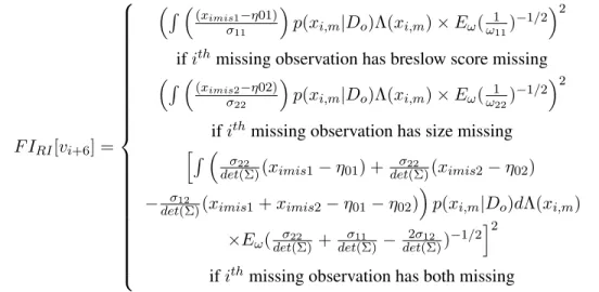
Forωmiss, wheni ∈ {1,2, . . . ,72}, which corresponds to the observations with one or two missing covariates, then

F IRI[vi+6] =                                             

R (ximis1−η01)

σ11

p(xi,m|Do)Λ(xi,m)×Eω(_ω1₁₁)−1/2 2

ifithmissing observation has breslow score missing

R (ximis2−η02)

σ22

p(xi,m|Do)Λ(xi,m)×Eω(_ω1₂₂)−1/2 2

ifithmissing observation has size missing h

R σ22

det(Σ)(ximis1−η01) + σ22

det(Σ)(ximis2−η02)

− σ12

det(Σ)(ximis1+ximis2−η01−η02)

p(xi,m|Do)dΛ(xi,m)

×Eω(_det(Σ)σ22 +_det(Σ)σ11 −_det(Σ)2σ12 )−1/2 i2

ifithmissing observation has both missing

(2.24)

Recall thatEω()is the expected value with respect top(Dc, ω), and the power is taken after the expected value. The FI forβand the missing observations have already been scaled in their expression.

Table 2.2: First order influence measures for E1684 data FI in direction of β1 β2 β3 β4 φ1 φ2

(40)

As we can see from the Table 2.2, there is only a small change in the curvature of the Bayes Factor as we scale the variance due to FI’s small value. Because we have put the theβ0son the same scale, the equivalent FI values show that there is noβthat is more influential than the others. This is mostly due to the fact that the hyperparameter for the variance of theβ0sis on the orders of magnitude larger than the mean of theβ0s.

Table 2.2 also suggests that there is only a minor change if we decided to take into account covariance between the log baseline hazards in the first and second window, however the covariance between the log baseline hazards in the second and third window has a large effect on the Bayes factor.

The missing data perturbation, as shown in Figure (2.2), shows a similar story. The FI values vary from 1.7e-4 to 85.1, which indicates not much influence over the Bayes factor. The 3 highest FI’s come from observations that are missing both covariates, but these values are not much higher than the other FI’s. The lack of high FI’s suggests that none of the observations is particuarly influential on the Bayes factor.

2.4 SIMULATIONS

To access the variability of the FI measures, we created 100 bootstrap iterations with sample size 285 (the original sample size) with replacement from the ECOG data and linked the FI measures back to the original observations. Figure 2.3 shows that the measure has a lot of variability and is dependent on the sample. An observation might have high FI in one bootstrap sample and low FI in another. Since this is the case, it is prudent to consider not only the original data’s FI, but also how high a percentage of the observations might be. To this end, we consider both the75th and90thpercentile.

We could consider an observation as having high influence if the observation had a large value in the original data set and the75thpercentile was above a certain cutoff. By forcing the75thpercentile to be above a certain cutoff implies that25%of the bootstrap sample is above the cutoff. The FI graph of the original values, Figure 2.2, suggests that 50 might be a reasonable cutoff. Figure 2.4, which shows the inter-quartile range versus the observation number overlayed with the original FI values, suggests that 30 might be a good cutoff for the75th _{percentile in this data set. Using this cutoff suggests that there 6 potential influential}

(41)

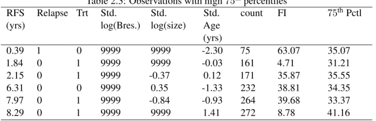
outliers (Table 2.4), all of which have both variables missing, while in the cutoff using the75thpercentile, there were some observations that only have Breslow missing. This suggests that the tails of the distribution of the FI measure could be related to the number of variables that are missing for a particularly observation. Using this cutoff, we see there are 5 observations whose original FI values are greater than 50 (observation numbers 75, 81, 156, 184, and 189) and whose90thpercentile is high.

Table 2.3: Observations with high75thpercentiles RFS

(yrs)

Relapse Trt Std. log(Bres.)

Std. log(size)

Std. Age (yrs)

count FI 75thPctl

0.39 1 0 9999 9999 -2.30 75 63.07 35.07

1.84 0 1 9999 9999 -0.03 161 4.71 31.21

2.15 0 1 9999 -0.37 0.12 171 35.87 35.55

6.31 0 0 9999 0.35 -1.33 232 38.81 34.35

7.97 0 1 9999 -0.84 -0.93 264 39.68 33.37

8.29 0 1 9999 9999 1.41 272 8.78 41.16

Table 2.4: Observations with high90thpercentile values RFS

(yrs)

Relapse Trt Std. log(Bres.)

Std. log(size)

Std. Age (yrs)

count FI 90th Pctl

0.26 1 1 9999 9999 -0.33 53 0.01 80.66

0.39 1 0 9999 9999 -2.30 75 63.07 68.07

0.44 1 1 9999 9999 1.10 81 63.17 63.58

1.70 1 1 9999 9999 -0.99 156 65.69 85.39

1.84 0 1 9999 9999 -0.03 161 4.71 95.77

3.02 1 1 9999 9999 0.32 184 4.93 97.37

3.28 1 0 9999 9999 -0.70 189 82.34 91.21

4.89 0 1 9999 9999 -0.52 210 85.13 71.85

8.29 0 1 9999 9999 1.41 272 8.78 151.09

1

The Tables 2.3 and 2.4 suggest that we have perhaps 1 observation whose75thand90thpercentile are different from the rest of the data, and whose original FI was high. However, this observation does not seem a cause for concern given the high variability of the FI measure.

1

RFS: Relapse Free Survival time Relapse is 1 if relapse occured

(42)

2.5 DISCUSSION

The purpose of performing model diagnostics is to ensure that the chosen model is not sensitive to small changes, and if the model is sensitive to small changes, we need to be forthwright with investigators about the model’s sensitivity. As investigators, we may be interested in changes that that are a result of our modeling or prior assumptions.

In this paper, we used both simulated data and a real data set to explore how our modeling and prior assumptions effected the Bayes factor. Our first simulation example explored perturbations to the model by perturbing the hazard function. By knowing the truth behind the simulations, we can verify that the diagnostics are accurately picking up perturbed observations. We see that the influence measures pick up big changes, and is not sensitive to smaller changes. For diagnostics, that is what we want as we are only interested in knowing about potential large changes to our model.

For our ECOG data set, we explored perturbations to the variances ofβ,φ, and the influence of individual observations. Our perturbation to the variances ofβand the covariances ofφrepresent perturbations to the prior assumptions. The FI measure forβ were largely dominated by the original hyperparameter variance forβ. In non-informative cases, the variance forβis chosen to be many orders of magnitude larger than the hyperparameter mean of β. Since the original hyperparameter for the variance of β appears in the denominator of the FI measure, it ends up dominating the term. No one variable is more influential in the model unless its estimate is large compared to the hyperparameter variance.

We see from our bootstrap sample of the ECOG data set, that the FI measure has much variability. It gives a sense that “large” FI should only be those whose order of magnitude are 2 to 3 times the majority of the data. Knowing this, we suspect that there are not any unduely influential observations in the ECOG data set.

(43)

(44)

Figure 2.2: First order influence measures for missing observations

(45)

(46)

(47)

CHAPTER 3: ROC ANALYSIS IN THE PRESENCE OF VERIFICATION BIAS

3.1 INTRODUCTION

Chronic obstructive pulmonary disease (COPD) is the fourth leading cause of death in the United States, affecting more than 5% of the adult population (Lin et al., 2008). Despite its high prevalence, COPD is not often diagnosed until it has reached advanced stages. According to the Global Initiative for Chronic Obstructive Lung Disease (GOLD), COPD is defined as air flow limitation that is not fully reversible, is gradually progressive, and is associated with an abnormal inflammatory lung response to noxious particles or gases (Rabe et al., 2007), making it hard to diagnose. Four out of five COPD patients have ever smoked or are current smokers, which puts smokers in a high risk population. Still there have been some attempts to screen the general population and not just high risk patients.

The main method of diagnosing a patient with COPD is office spirometry. When the subject blows into an office spirometer, it measures variables such as the forced expiratory volume in 1 second (FEV1) and forced volume capacity (FVC) and assigns a quality grade (A-F) that indicates the validity of the reading. A passing grade (A-C) is sometimes difficult to achieve for patients who have to blow into the device for as long as 10 seconds. Enright and Kaminsky (2003) suggest that instead of asking general practitioners to do spirometry, technicians should perform the test and then have general practitioners interpret the results.

(48)

lower limit of normal for FEV1/FVC for different populations. In the end, the significant covariates in the equations were gender, height, race, and age. With so many ways of defining a COPD case, estimates for population prevalence vary. Some reports calculate a COPD prevalence of 4.5% while others calculate a 21.1% prevalence (Wilt et al., 2005).

With all the difficulties of using spirometry to determine COPD, the U.S. Preventive Services Task Force (USPSTF) was formed in order to make a recommendation on whether using spirometry to screen for COPD is effective. The USPSTF reviewed COPD studies from 1966 to 2007. Lin et al. (2008) did a review of the studies and found no papers provided direct evidence on health outcomes associated with screening for COPD. They concluded that screening using spirometry would require testing hundreds of patients to identify a single exacerbation and would likely identify people with mild or moderate airflow obstruction who would not experience any adverse health benefits attributable to COPD, and was therefore not an effective screener for COPD in the general population.

Since the Agency for Healthcare Research and Quality (AHRQ) did not recommend spirometry for COPD screening (Qaseem et al., 2007; Lin et al., 2008) for healthy adults who do not report symptoms to a clinician, there has been a need to develop and evaluate alternatives to spirometry for detecting COPD. Nelson et al. (2012) staged a large COPD screening study in the general adult population to evaluate pocket spirometers. Ideally, screening tools should be affordable, simple, and accurate enough to avoid producing large numbers of false positives or false negatives (Marshall, 1996a,b). Pocket spirometers cost approximately $30 and require a short exhalation, making them ideal for large screening studies of the sort described in Nelson et al. (2012). These devices, however, have not been validated for accuracy as a population-wide screener. Both FEV1 and peak expiratory force (PEF), which is the maximum speed of exhalation, can be measured with a pocket spirometer. Nelson et al. (2012), selected PEF as the measurement to be used for screening in their general population study. The main question of interest is whether there is a significant difference between the performance of the pocket spirometer screener on PEF and FEV1 when used on the entire population of interest, and not just the study population.