A new approach for the automatic detection of shear-wave splitting

(1)

A New Approach for the Automatic Detection of

Shear-wave Splitting

by Yang Zhao

A thesis submitted to the faculty of the University of North Carolina at Chapel Hill in partial fulfillment of the requirements for the degree of Master of Science in the Department of Geological Sciences.

Chapel Hill

2008

Approved by

Advisor: Jose A. Rial

(2)

ii ©

2008 Yang Zhao

(3)

ABSTRACT

YANG ZHAO

A New Approach for the Automatic Detection of Shear-wave Splitting

(Under the direction of Professor Jose A. Rial)

This thesis introduces a new approach for the automatic detection of two crucially important shear wave splitting (SWS) parameters, fast wave polarization and delay time between split waves, from microearthquake seismograms. The method is based on the

analyses of multiple time windows that include the shear wave arrivals. An automated SWS algorithm is performed for each specified window. Over the estimates of the two parameters (polarization and time delay) obtained from all windows, an unsupervised

cluster analysis is applied to locate the region with the most stable estimate. The optimal region is that with the lowest variance. The mean value of the optimal cluster is regarded as the best estimate of polarization and time delay. The estimates are relatively easy to derive from large seismic datasets and show high reliability. We compare the results with

(4)

iv

ACKNOWLEDGEMENTS

I would like to thank my advisor Dr. Jose Rial. His supervision and advice is invaluable. Dr. Jonathan Lees and Dr. Kevin Stewart served as committee members and helped me with their comments and questions.

I would especially like to thank my Dad and Mom for their support.I would like to thank the faculty, staff, and graduate students in the Department of Geological Sciences as well for their support during my years at Carolina.

(5)

LIST OF TABLES

Table 1: Parameter table for the automatic detection code on

(7)

LIST OF FIGURES

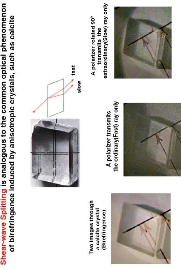
Figure 1.1: Illustration of shear wave splitting by the common optical

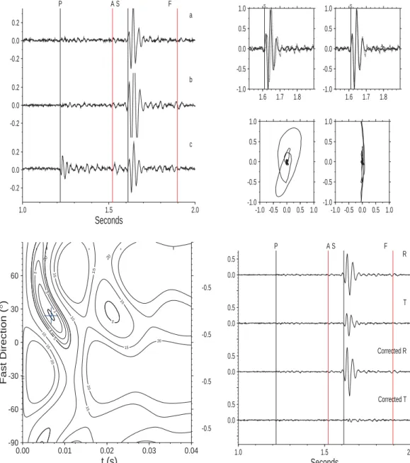
birefringence induced by anisotropic crystals………..………3 Figure 1.2: The standard correction measurement of polarization and

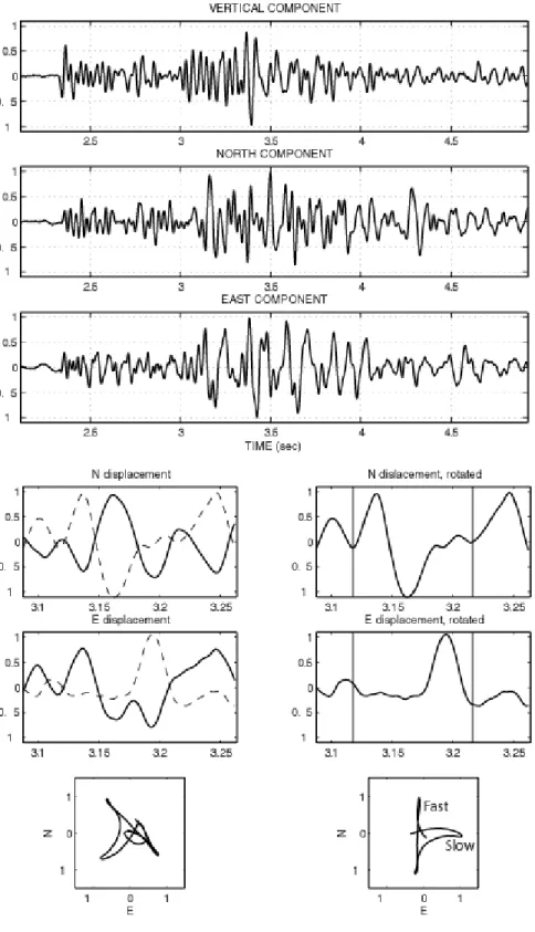
delay time from the recorded seismogram………..……..6 Figure 1.3: Cross-correlation measurement of polarization and delay

time from the recorded seismogram……….7 Figure 2.1: The window selection of shear wave splitting analysis,

seismogram samples for the NW Geysers……...………..11 Figure 2.2: The AIC function is calculated for both components

from a real seismogram in the original coordinate…...……….13

Figure 2.3: Seismogram from Figure 2.2 in a rotated coordinate

system………....….14 Figure 2.4: The calculated AIC functions for both components

of a sample seismogram from the NW Geyser……….….15 Figure 2.5: Estimates of delay time and polarization three hundreds

of different analysis windows………...…….17 Figure 2.6: The algorithm flow chart of the main flow of shear wave

splitting analysis procedure………...……….21 Figure 2.7: The algorithm flow chart of Auto_SWS program………...……..23 Figure 2.8: The algorithm flow chart of Revised AIC Picker program………...…….26

Figure 3.1: The locations of the seismic stations and recorded

microearthquake in NW and SE Geysers………...………29 Figure 3.2: Rose diagrams showing fast shear wave polarization

recorded in NW Geysers………30

Figure 3.3: Rose diagrams showing fast shear wave polarizations

recorded in SE Geysers, CA in 1999………...……….31 Figure 3.4: The Location of Hengill geothermal reservoir in active

(8)

viii

August 12th in Hengill, Iceland………...…………..35 Figure 3.6: Rose diagrams showing the fast shear-wave polarization

directions in Hengill, Iceland……….………36 Figure 3.7: The seismicity recorded by the Coso array from 2005

January to 2006 September………39 Figure 3.8: Rose diagrams showing the fast shear-wave polarization

directions observed 48A-19RD area………...………40 Figure 3.9: Comparison of the results from manual picks with those

(9)

INTRODUCTION

Shear-wave Splitting

Since the discovery of seismic anisotropy in the oceanic mantle (Hess, 1964), seismologists have been attempting to characterize it in crust and mantle. One of the most powerful and successful methods to study fracture-induced anisotropy is to investigate

split shear waves that travel through these layers (Crampin, 1993).

It is known that a shear-wave propagating through rocks with stress-aligned micro-cracks (also known as extensive dilatancy anisotropy or EDA-cracks) will split into two waves, a fast one polarized parallel to the predominant crack direction, and a slow one, polarized perpendicular to it (Crampin, 1981, 1984; Babuska and Cara, 1991).

The phenomenon is very similar to optical birefringence, whereby light transmitted through an anisotropic crystal undergoes analogous splitting and polarization parallel and perpendicular to the alignment of atoms in the crystal lattice, which is illustrated by Figure 1.1. In the seismic case, the polarization direction of the fast split shear wave parallels the strike of the predominant cracks regardless of its initial polarization at the

(10)

2

1991). Measuring the fast-shear wave polarization and time delay from local microearthquakes has thus become a valuable technique to detect the orientation and intensity of fracturing in the subsurface of fracture-controlled geothermal field (e.g. Lou

and Rial, 1997; Vlahovic et al., 2002a,b; Elkibbi and Rial, 2003, 2005; Elkibbi et al., 2004, 2005; Yang et al., 2003; Rial et al., 2005; Tang et al., 2005).

Applications of the shear-wave splitting technique to geothermal fields have been extensively documented (e.g. Lou and Rial, 1994, 1995, 1997; Rial and Lou, 1996; Lou et al., 1997; Erten and Rial, 1998, 1999; Vlahovic et al., 2001). Although in principle

straightforward, the analysis of shear- wave splitting for the purpose of crack detection is laborious, requiring careful processing of a large number of 3-component seismograms from all azimuths around every station. This is because a number of undesirable effects, such as the presence of multiple orientations of cracks between source and receiver,

complicated earthquake source time history, strong medium heterogeneity, thick weathered surface layer or rugged surface topography, among others, may strongly distort the signal, making the identification of crack-induced splits difficult to impossible. The correct measurement polarization and delay time often requires experience, diligence and

dedication for the task is very time consuming. It is therefore a seismologist’s dream to develop new skills to accomplish the measurement automatically, ultimately simplifying the monitoring of the field's subsurface crack system during exploration and into production

(11)

(12)

4

Measuring Polarization and Time Delay

Traditional techniques to extract polarization and delay time information from split seismograms are based on cross-correlation of two horizontal components and the standard correction method of Silver and Chan (1991).

In the standard correction method, first, a shear-wave analysis window is defined, which is normally picked manually. If anisotropy is present the particle-motion within this window will be elliptical. Second, a grid search over polarization and delay time is performed, where both components are rotated by polarization and one component is

lagged by delay time. The result which has the lowest second eigenvalue of the corrected particle-motion covariance matrix indicates linear particle motion after correction and is the solution which best corrects for the splitting. An F-test is used to calculate the 95%

confidence interval for the optimum values for polarization and delay time. After the splitting correction has been applied the method requires that the corrected waveforms in the analysis window match. The second eigenvalue of the particle motion covariance matrix provides a measure of this match. The smaller the second eigenvalue, the better the match (Teanby et al., 2003). (see sample in Figure 1.2) A good result will have a

unique solution. Criteria for reliable results are discussed in Savage (1999) and Silver and Chan (1991).

(13)

plot shows that fast and slow shear-waves are oriented along the instrument’s horizontal components. The angle of rotation from the original polarization direction determines polarization. At the same time, the two shear-wave arrivals, which are often coupled in

(14)

6 -1.0 -0.5 0.0 0.5 1.0

-1.0 -0.5 0.0 0.5 1.0 -1.0 -0.5 0.0 0.5 1.0

-1.0 -0.5 0.0 0.5 1.0 -1.0

-0.5 0.0 0.5 1.0

1.6 1.7 1.8

S -1.0 -0.5 0.0 0.5 1.0

1.6 1.7 1.8

S -0.5 0.0 0.5 -0.5 0.0 0.5 -0.5 0.0 0.5 -0.5 0.0 0.5

1.0 1.5 2.0

Seconds

P AS F

R T Corrected R Corrected T -0.2 0.0 0.2 -0.2 0.0 0.2 -0.2 0.0 0.2

1.0 1.5 2.0

Seconds

P AS F

a b c 5 5 10 10 10 15 15 15 15 15 15 20 20 20 20 20 -90 -60 -30 0 30 60

Fast Direction (

°

)

0.00 0.01 0.02 0.03 0.04

t (s) 2 3 3 4 5 5

(15)

(16)

8

Both methods require the manual selection of an appropriate time window by the operator, which is time consuming, introduces subjectivity, and usually influences the results. Automatic detection of shear wave splitting was attempted by Savage et al (1989).

The disadvantage of their methods is that they do not address the effect that different shear-wave analysis time windows can have on the results. Teanby et al. (2003) used cluster analysis to remove subjectivity of window selection. However, their method needs manual quality control with diagnostic plot, which can still be human biased and

laborious.

Current seismic deployments aim for multiple geophone arrays and longer recording times. Correspondingly, data volumes from microseismic and teleseismic are

growing quickly in recent years. These large datasets provide insights into lithological properties, making it possible to constrain fracturing and intrinsic anisotropy. But manual analysis of each event easily becomes an endless job, consequently plagued by operator errors.. This facts are forcing seismologists to engineer automated approaches without

human involvement.

Here I introduce a novel method of automatic detection of shear wave splitting parameters, which extends the idea of automated window selection by Teanby (2003),

(17)

providing a convenient approach to process such huge seismic datasets automatically and objectively. In Chapter 2 we discuss the shear wave analysis window selection and compare two different splitting techniques with the Automatic SWS algorithm proposed

by this paper, and then show the clustering algorithm and an optimized cluster choosing procedure as well as the best estimate selection process. In Chapter 3, the results of our Automatic SWS algorithm are shown using observational data collected from The Geysers and Coso, CA and Hengill, Iceland geothermal fields. We illustrated how the

(18)

METHODOLOGY & PROGRAM DESCRITPTION

WINDOW SELECTION

Finding the optimal shear wave time window for the detection of SWS parameters depends on critical factors such as adequate S/N ratio in the shear wave, and enough length to include several periods of the dominant frequency. It is however quite time consuming and subjective to find the optimal window manually, by visual inspection. On

the other hand, it is well known that the actual shear wave splitting process is stable with respect to the noise (Teanby et al., 2003). Therefore, it is very important to ensure that the splitting parameters are stable over a wide range of different window lengths and intervals. This steadiness guarantees the robustness of measurement and minimizes the

effects of noise. The method introduced here achieves this by considering a large number of analysis windows to look for stable regions in the space of solutions, that is, in polarization and time delay space.

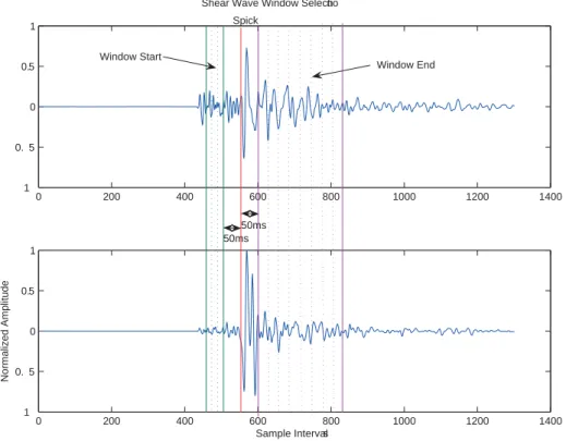
The method proceeds as follows: First, a set of shear wave analysis time windows

are constructed as illustrated in Figure 2.1. The Start window is selected at T_begin and will

vary from T_begin_{_ 0} to T_begin_{_1} with N_begin steps of dT_beginlength. Similarly, the End window

is selected at T_end varying from T_end_{_ 0} to T_end_{_1} with steps N_end of dT_end length. The total

(19)

N_total =N_begin×N_end (1)

where T_begin and T_end are all defined relative to the onset of the shear wave.

Refer to Table 1 in Chapter 3 for typical numerical values of the window parameters

applied on microseimic datasets.

0 200 400 600 800 1000 1200 1400

1 0. 5

0 0.5 1

0 200 400 600 800 1000 1200 1400

1 0. 5

0 0.5 1

Sample Intervals

Normalized Amplitude

Shear Wave Window Selection

Window Start

Window End Spick

50ms 50ms

Figure 2.1. The red line indicates the shear wave onset. The solid green line indicates the start of shear wave analysis window, while dashed green lines indicate a number of possible window starts. Similarly, the purple lines indicate the window ends. The distance between the closest window start/end and shear wave pick is 50 sample intervals for this example from The Geyseys.

SPLITTING ALGORITHM

(20)

12

Once the shear wave analysis windows are selected, the splitting algorithm used to determine polarization and time delay is applied to each window. We estimate the value of polarizations and delay times by making use of existing automatic wave arrival

picking techniques. The algorithm used is the AIC (Akaike Information Criteria) picker by Maeda (1985), which calculates the AIC function directly from the seismograms. The onset is the point having the minimum AIC value. For the seismogram x[k] (with k=1, 2…N) of length N, the AIC value is defined as

AIC k( )= ×k log{var( [1, ])} (x k + N− − ×k 1) log{var( [x k+1,N])} (2)

where k ranges through all the seismogram samples.

The idea of this algorithm is to use the well known automatic picking algorithm to detect significant arrival time difference (here “significant” means the difference between the arrival times of the fast and slow shear waves within 10 to 60 sampling intervals (see

Section 4 for details) between the two horizontal components in a rotated coordinate system. In order to search the entire coordinate span, the algorithm rotates the two horizontal components of the seismograms from 0 to 180 degrees by one-degree increments. During each incremental rotation of the coordinate axes, the variance of the

interval (between fast and slow arrival times in the window) in the slow component is calculated. The polarization will be the angle corresponding to the rotated coordinate in which the differential arrival time is significant and the variance in the slow component reaches its minimum (meaning the slow component in that interval is most quiescent).

(21)

0 50 100 150 −1

0 1

E

0 50 100 150

−300 −200 −100

AIC

0 50 100 150

−1 0 1

N

0 50 100 150

−300 −200 −100

AIC

9406051424 (Before Rotation)

global minimum=88

global minimum=84

Figure 2.2. The AIC function is calculated for both horizontal components from a real seismogram in the original coordinate. The vertical lines indicate the onset times of the waves. The differential arrival time is not significant (<10) in this coordinate.

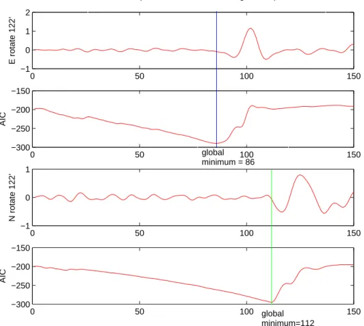
Illustrative results of the AIC picker algorithm are shown in Figure 2.3. As

(22)

14

0 50 100 150

−1 0 1 2

E rotate 122’

0 50 100 150

−300 −250 −200 −150

AIC

0 50 100 150

−1 0 1

N rotate 122’

0 50 100 150

−300 −250 −200 −150

AIC

9406051424(After Rotation, Rotated Angle=122’ )

global minimum = 86

global minimum=112

Figure 2.3.Seismogram from Figure 2.2 in a rotated coordinate system. The difference of two arrival times between the two components is 26 sampling intervals, and rotating angle is 122 degree.

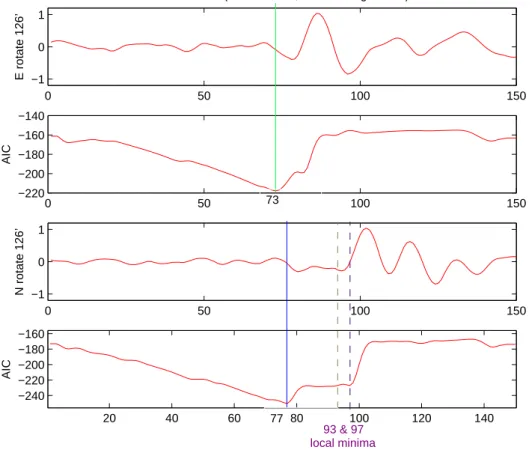
Revised AIC Picker

When there is more noise than signal or multiple seismic phases in a time window

(23)

using the simple AIC picker technique. Figure 2.4 shows that the method sometimes yields erroneous answers to the arrival times for low S/N ratio seismograms.

0 50 100 150

−1 0 1

9403062006 (After rotation, Rotated Angle=126’)

E rotate 126’

0 50 100 150

−220 −200 −180 −160 −140 AIC

0 50 100 150

−1 0 1

N rotate 126’

20 40 60 80 100 120 140

−240 −220 −200 −180 −160 AIC 73 77

93 & 97 local minima

Figure 2.4. The calculated AIC functions for both horizontal components from a seismogram. The green and blue vertical lines indicate the onset times of the waves defined by the global minima of the AIC functions, while the purple and yellow dash lines represent the possible onset times suggested by the local minima.

The problem in Figure 2.4 is that before the slow wave arrives, the north component is disturbed, probably by the arrival of a scattered wave, and the AIC picker

(24)

16

In order to avoid that scattered or noise disturbances be regarded as signals, we take the global minimum value and local minima into account simultaneously while rotating the components of the seismogram.

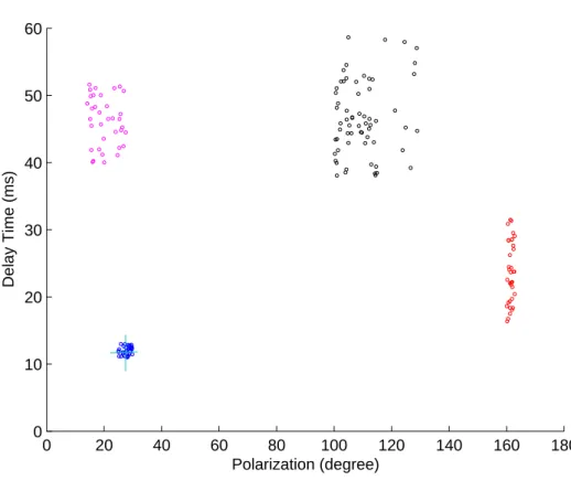
CLUSTERING ALGORITHM

Once the Automatic Splitting Algorithm is applied on each shear-wave analysis

window, it results in a set of N_total estimates of polarization and delay time. With the

purpose of varying the analysis window and looking for robust values in polarization and

delay time, we plot the Ntotal pairs of polarization and delay times in a 2D plane. These

(25)

0 20 40 60 80 100 120 140 160 180 0

10 20 30 40 50 60

Polarization (degree)

Delay Time (ms)

Figure 2.5. （synthetic） Estimates of delay time and polarization from three hundreds of different analysis windows. The estimates condense into tight clusters of points. Many points in the clusters lie on top of each other because delay time and polarization are found using a grid search. Different colors represent different cluster

Since the polarization and delay time are on different scaled units (degree and

sampling intervals), we need to normalize the data in order to eliminate different weight effects on the polarization and delay time caused by the clustering algorithm. According to our microearthquake datasets, we define the standardized range for polarization and delay time as 180 degree and 60 sampling intervals, respectively. Scaling by this variable

range has performed very well in many clustering applications (Teanby et al., 2003; Everitt et al., 2001; Milligan and Cooper, 1985 ,1988).

(26)

18

unsupervised technique is required to identify these clusters by reason of the automated requirements. Here we use Density-Based Scan Algorithm with Noise (DBSCAN) (Ester et al., 1996) to identify clusters and determine optimal cluster number. DBSCAN typically

regards clusters as dense regions of objects in the data space which are separated by low density regions. DBSCAN is a density-based clustering technique which starts from an arbitrary object, and if the neighborhood around it within a given radius (Eps) satisfies at least the minimum number of objects (MinPts), this object is a core object, and the search

recursively continues with its neighborhoods and stops at the border objects where all the points within the cluster must be in the neighborhood of one of its core objects. Another arbitrary ungrouped object is selected and the process is repeated until all data points in the dataset have been placed in the clusters. All the non-core objects which are not in the

neighborhood of any of the core objects are labeled as noise. DBSCAN doesn’t need the number of final clusters to be given in advance where it automatically detects dense regions and its output is the natural number of clusters. (Daszykowski et al., 2001). Four clusters are shown in Figure 2.5 represented with different colors.

Once the clusters are identified by the DBSCAN algorithm, we need to determine the optimal cluster, and then the best estimate from the optimal cluster. The criterion to determine the optimal cluster depends on the number of data points and the variance

within each cluster. To implement the criteria, we define N_cluster_{_ min} if one cluster with

less than N_cluster_{_ min} data points is being regarded as noise. N_cluster_{_ min} Correspond to

approximately a cycle’s worth of points, which is normally less than the total number of

(27)

The within cluster variance σ2j is calculated according to

( ) 2 ( ) 2

( ) ( )

2 1( ) 1( )

j j

N j N j

j j i i i i j j t t N δ φ σ − −

= − + = − Φ

=

∑

(3)

Where δti( )j and

( )j i

φ are the ith results of delay time and polarization, respectively,

which belong to cluster j. N_j is the number of points in cluster j.

The mean position of points within each cluster is defined as

( ) 1 ( ) ( ) 1 ( ) j j N _j i i j j N _j i i j j t t N N δ φ − = − = = Φ =

∑

(4)

Therefore, the optimal cluster is found in the cluster with the smallest variance ( 2

j

σ ). The

best estimate is the mean value of δt and φ of the optimal cluster. The best estimate

(28)

20

According to the suggestions from my master defense in May, 8th, 2008, here I attached 18 cluster plots from the real mircoseismic dataset(The first three from Coso, The second three from The Geysers , and the last three from Hengill)

(29)

(30)

22

(31)

Figure 3.0(b) Coso event –20060702024436, the same symbol & color plot as Figure

(32)

24

(33)

Figure 3.1(b) Coso event –20060712081726, the same symbol & color plot as Figure

(34)

26

(35)

Figure 3.2(b) The Geysers event – 9403032027, the same symbol & color plot as Figure

(36)

28

(37)

Figure 3.3(b) The Geysers event –9402030208, the same symbol & color plot as Figure

(38)

30

(39)

Figure 3.4(b) The Geysers event –9403240234, the same symbol & color plot as Figure

(40)

32

(41)

Figure 3.5(b) Hengill event –2005072206145, the same symbol & color plot as Figure

(42)

34

(43)

Figure 3.6(b) Hengill event –2005072807484 , the same symbol & color plot as Figure

(44)

36

(45)

Figure 3.7(b) Hengill event –2005080602591, the same symbol & color plot as Figure

(46)

38

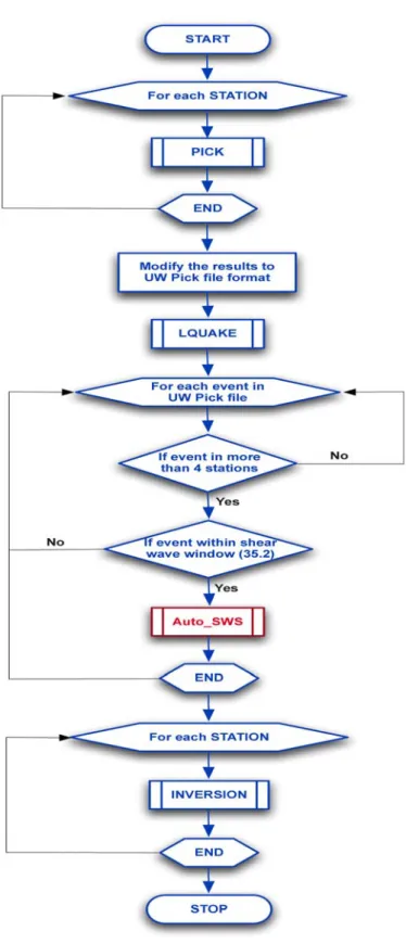
Algorithm Flow

Three flow charts depicted below aim to describe every single step of the

Auto_SWS program introduced in this chapter. First of all, it is necessary to discuss briefly about the main flow of the shear wave splitting analysis, as illustrated in Figure 2.6. We begin the analysis with picking P-wave arrival times and S-wave arrival times of each seismogram for each station. Seismic events are located by using a standard iterative

non-linear inverting algorithm (LQUAKE) based on Geiger’s method to determine origin time and hypocenter of an earthquake from P-wave arrival times. In most cases, as the iteration proceeds, the solution vector will converge till the error is within some preset tolerance. As for low S/N ratio case, hypocentral locations by only using P-wave readings

are not very reliable. Therefore, we used both P- and S-wave arrival times when necessary. (Rial et al., 2007).

One qualified event in UW pick file has to display large signal to noise ratio,

(47)

(48)

40

shear-wave window. The angle is defined by the critical angle Ic=

1

( s/ p)

Sin− V V , where

p

V and V_s are the P-wave and S-wave surface velocities, respectively. Crampin (1981)

shows that when incident angles (measured from the vertical) are greater than I_c

shear-waves tend to interact strongly with the free surface, which contaminates the incoming

waveform with converted phases. Normally, the calculated Ic for our geothermal datasets

is approximately35o, verified by our former papers. (e.g. Lou and Rial, 1997; Vlahovic et al., 2002a,b; Elkibbi and Rial, 2003, 2005; Elkibbi et al., 2004, 2005; Yang et al., 2003; Rial et al., 2005; Tang et al., 2005).

Once qualified seismic events are selected, they will proceed to Auto-SWS

program as shown in the red rectangle (see detail in Figure 2.7) in Figure 2.6. The methodology of this program is described previously in this Chapter, so we only discuss several key steps.

As mentioned before, slight changes in the analysis window can cause very different solutions due to the cycle skipping effect, accordingly the selection of shear wave analysis window turns out to be a specific step. (Teanby et al,. 2003) Important

parameters areN_begin,N_end , dT , T_begin_{_1} and T_end_{_ 0}. Large N_begin N_end, small dT afford

abundant space for the grid search by the splitting algorithm, however it also requires a

huge computational time. Since the splitting estimates are much more sensitive to

window start rather than window end, we typically choose N_end 20-30 times more than

begin

(49)

(50)

42

Minimum window – the distance between the closest window start/end and shear wave

pick is defined by T_begin_{_1} and T_end_{_ 0} . The splitting algorithm (Revised AIC Picker)

requires a clear, integrated shear wave arrival and separates S phases from other phases which have different amounts of splitting. To satisfy these requirements, we define 50

sample intervals to be the minimum window. dT is not a critical parameter in this study,

as long as there are large enough range analysis windows and include the duration of shear wave energy envelop, which guarantee the robustness of the final results.

Although our method is much less sensitive to the influence of the cycle skipping

rather than other automated methods, the cycle skipping/window dependence effect is still a severe problem for band limited data. It’s also affected the comparison of the first and the second best cluster, where the first two best clusters provide 95% correct estimate

during our application to the selected geothermal datasets. If the first is obviously better than (both in the point number and the variance within the cluster) the second then the result is reliable, otherwise results may be affected by cycle skipping.

Similar to other automated methods, the Auto_SWS method still can not entirely make a distinction between null and other measurements. However, several features of our programs help us to overcome this problem. The first one is setting the upper and low limits for the intervals of delay time, ranging from 10 to 60 sampling intervals. Another

(51)

It’s consequently rejected by the cluster identification and the interval length control

The Revised AIC Picker served as the splitting algorithm is performed for every

specific analysis window, as shown in red rectangle (see detail in Figure 2.8) in Figure 2.7. Please refer to section 2 for detail.

(52)

44

(53)

APPLICATIONS

Data Description

The raw data used in my research are seismograms of micro-earthquakes traveling through the crack-induced anisotropic upper crust in The Geysers and Coso, CA, and

Hengill, Iceland geothermal reservoir fields. The anisotropic parameters measured manually from these seismograms, namely fast directions and delay times, compose the shear-wave splitting data used in my study. Although the manual detection of the anisotropic parameters inescapably adds extra random errors into the dataset to some

extent, it still substantially increases the overall reliability of the shear-wave splitting data since current detection methods that are fully automatic are not as accurate as manual detection.

The Geysers reservoir is the world’s largest commercially exploited dry-steam vapor-dominated geothermal field. The Geysers reservoir is located northeast of the San Andreas Fault in the northern Coast Ranges of California about 150 km north of San Francisco. The seismic waveforms analyzed for shear-wave splitting were recorded by

two seismic arrays deployed in the NW and SE Geysers regions by the Lawrence Berkeley National Laboratory (LBNL).

(54)

micro-46

geophones recorded at 400 sample/sec and were buried about 30 meters below the ground surface (Figure 3.2).

The SE Geysers is also seismically active with an average of 20 micro-earthquakes per day. Events are generally shallower than 4 km. The data were recorded

by a 12-station, 3-component, high frequency (480 samples per sec) digital network (Figure 3.3). All 12 stations had geophones on the ground surface, which did not perceptibly affect the quality of the seismic data in comparison with the NW buried instruments, as noise levels contained in the data were generally relatively low. (Elkibbi

(55)

Figure 3.1 The locations of the seismic stations and recorded microearthquake in NW and SE Geysers. (Elkibbi and Rial 2003)

(56)

48

(57)

Iceland is situated on top of the Mid-Atlantic Ridge where the ridge interacts with the Iceland Hot Spot. Several volcanic centers, active and extinct, are located within the island. One of them is the Hengill volcanic center which lies on the plate boundary

between the North America and the European crustal plates in Southwestern Iceland. The Hengill central volcano and its transecting fissure swarm, extending 70—80 km long from the coast south of Hengill to north of Lake Thingvallavatn with an associated graben structure, form the Hengill volcanic system, as depicted in Figure 3.4

Between July 2nd and August 12th, a 21-station, 3-component seismic array was deployed to the south of the Hengill central volcano, covering an area approximately 5 km in N-S by 10 km in E-W. The array continuously recorded the seismic activity in the

study area for forty-two days. The data were collected continuously at a rate of 500 samples per second. During the forty-two days of operation the array detected an average of 3 to 4 well-recorded events per day (observed at 5 or more stations). These are very small earthquakes with magnitudes probably no greater than 2. Figure 3.5 shows the

epicenters of the earthquakes located within and in the vicinity of the array from July 5th to August 12th. Also depicted in Figure 3.5 is the distribution of these seismic stations.

The data from seven selected stations in the eastern part of the array (H70—H76)

(58)

shear-50

(59)

(60)

52

Figure 3.5 The seismicity recorded by the array from July 5th to August 12th is shown. Totally 146 events are detected and 130 events properly located. (Hengill, Iceland) .(Tang et al., 2006)

(61)

(62)

54

The Coso geothermal is located along the eastern front of the Sierra Nevada, south western Basin and Range Province, California. It is situated to the east of the Sierra Nevada Frontal Fault in southern Owens Valley. (Duffield et al., 1980). The tectonics of

the Coso range are the reflection motion of a stress field influenced by the right slip San Andreas Fault system and the extensional Basin and Range environment. Three major classes of faults extensively fracture the area. The west-northwest-trending faults with right-lateral strike-slip motion are common in the southern and northwestern parts of the

geothermal field. North-northeast-trending normal faults with a small component of strike slip are prevalent within the geothermal field, while northeast-trending strike-slip faults with left-lateral sense of motion are well developed in the northeast part of the field (Roquemore, 1980;).

The Coso area is one of the most active seismic regions of southern California. Most of the events below the field are less than 3 km deep and are surrounded by deeper regional seismicity (down to 12 km depth). During the months of January 2005 and

August 2006, we studied these microearthquakes before, during and after this fluid injection tests at Well 46A-19RD area .A large number of high-quality seismograms from local microearthquakes in Coso recorded by a permanent, station, downhole, 3-component seismic array running at 500 samples per second.

(63)

time delay. Similarly with Hengill and The Geysers geothermal research, the Coso stations are selected to ensure that most of the earthquakes fall into the shear-wave window, a right circular cone with vertex at the station and vertex angle equal to 35° of

(64)

56

Figure 3.7 The seismicity recorded by the Coso array from 2005 January to 2006

(65)

(66)

58

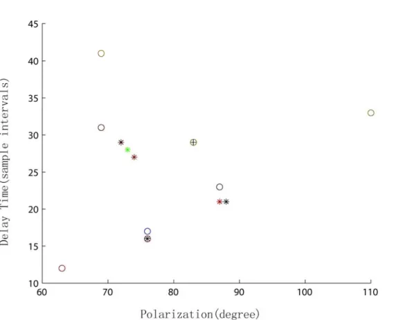
Comparison of Estimate Results

Availability of previous reliable splitting measurements, diverse subsurface structural settings, event depths and qualities of the seismic data make these datasets a

good test case opportunity for our Automatic SWS Algorithm.

Figure 3.9 summarizes the comparison between the manual results and the results from three different splitting algorithms (See Chapter 2) by using the automated window

selection method. Figure 3.9 (A) obtained from the traditional cross-correlation method. (See detail in Chapter 1). However, the solutions do not satisfy the requirements for reliable splitting estimates as illustrated in Figure 3.9 (A). The unreliable estimate results after implementing the AIC picker method are much reduced in Figure 3.9 (B), but still

about one third of these estimates are outside of error tolerance .To achieve better reliability, the AIC picker is revised to serve as our Automatic SWS algorithm works best among the manual results and automated estimates as shown in Figure 3.9 (C). About 76/80 of polarization estimates and 70/80 of delay time estimates are inside the tolerance

(67)

0 50 100 150 0 50 100 150 Manual

Revised AIC Picker

Polarizatio n 0 20 40 60 80

0 20 40 60 80

Manual

Revised AIC Picker

Delay Time(sample intervals)

0 50 100 150 0 50 100 150 Manual AIC Picker Polarizatio n 0 20 40 60 80

0 20 40 60 80

Manual

AIC Picker

0 50 100 150 0 50 100 150 Manual Cross Correlation Polarizatio n 0 20 40 60 80

0 20 40 60 80

Manual

Cross Correlation

(A)

(B)

(C)

(68)

CONCLUSION

This thesis illustrates a novel approach for the automatic, real-time detection of shear-wave splitting parameters. In contrast with previous methods, I have developed three major improvements: dramatically increasing data processing speed of shear wave

splitting, successfully avoiding the subjectivity of window selection by using an objective automated window selection, and removing the dependence of results on manual quality control.

The method requires travel time picks for the S phase as well as a set of windowing and clustering parameters. The parameters in our method are given in Table 1. Parameters were chosen based on the main influencing factors on the quality of estimates, such as seismic S/N ratio and sampling rate.

This approach can be used to improve the quality of shear wave splitting analysis and is especially suited to large datasets. For Coso and The Geysers geothermal datasets,

each event took half minute to process on a single 2GHz processor.

The approach has been successfully applied to the shear wave splitting data obtained from The Geysers and Coso, California and Hengill, Iceland geothermal fields,

(69)

Parameter Value

_1

begin

T 50 ms before shear wave pick

_ 0

end

T 50 ms after shear wave pick

begin

dT 25

end

dT 10

begin

N 3

end

N 20

Eps 0.8

MinPts 10

_ min

cluster

N 25

(70)

62

REFERENCES

Adams, M.C., Beall, J.J., Hirtz, P., Koenig, B.A., and Bill Smith, J.L., 1999. Tracing effluent injection into the SE Geysers-a progress report, Transactions, Geothermal Resources Council: 341-345.

Babuska, V. and Cara, M. (1991), Seismic Anisotropy in the Earth, Modern Approaches in Geophysics, Vol. 10, pp. 217, Kluwer Academic Publishers, The Netherlands.

Booth, D.C. and Crampin, S. (1985), “Shear-wave polarizations on a curved wavefront at an isotropic free-surface”, Geophys. J. Roy. Astr. Soc., 83, 31-45. Brandsdóttir, B., Menke, W., Einarsson, P., White, R.S., and Staples, R.K. (1997),

“Faroe-Iceland Ridge Experiment 2. Crustal structure of the Krafla central volcano”, J. Geophys. Res., 102, 7867-7886.

Crampin, S. (1981), “A review of wave motion in anisotropic and cracked elastic media”, Wave Motion, 3, 343-391.

Crampin, S. (1984), “An introduction to wave propagation in anisotropic media”,

Geophys. J. Roy. Astr. Soc., 76, 17-28.

Crampin, S., Booth, D.C., Krasnova, M.A., Chesnokov, E.M., Maximov, A.B., and Tarasov, N.T. (1986), “Shear-wave polarizations in the Peter the First range indicating crack-induced anisotropy in a thrust-fault regime”, Geophys. J. Roy. Astr. Soc., 84, 401-412.

Crampin, S. (1987), “Geological and industrial implications of extensive dilatancy anisotropy”, Nature, 328, 491-496.

Crampin, S. and Lovell, J.H. (1991), “A decade of shear-wave splitting in the Earth’s crust: What does it mean? What use can we make of it? And what should we do next?” Geophys. J. Int., 107, 387-407.

Crampin, S. (1993), “A review of the effects of crack geometry on wave propagation through aligned cracks”, Can. J. Expl. Geophys., 29, 3-17.

Daszykowski, M., Walczak, B. and Massart, D.L.(2001), Looking for natural patterns in data: Part 1. Density-based approach. Chemometrics and Intelligent Laboratory Systems. v56 i2. 83-92.

Elkibbi, M. and Rial, J.A. (2003), “Shear-wave splitting: an efficient tool to detect 3D fracture patterns at The Geysers, California”, Proc. Geothermal Reservoir Engineering, Stanford, 28, 143-149.

(71)

with shear-wave splitting”, Geothermal Resources Council (GRC) Transactions, 28, 789-800.

Elkibbi, M., Yang, M., and Rial, J.A. (2005). “Crack-induced anisotropy models in The Geysers geothermal field”, Geophys. J. Int., 162, 1036-1048.

Elkibbi, M. and Rial, J.A. (2005), “The Geysers geothermal field: Results from shear-wave splitting analysis in a fractured reservoir”, Geophys. J. Int., 162, 1024-1035. Everitt, B., Landau, S., Leese, M. (2001), Cluster Analysis, 4th ed., Edward Arnold,

London,

Ester M., Kriegel H.-P., Sander J., Xu X.(1996): “A Density-Based Algorithm for 17

Discovering Clusters in Large Spatial Databases with Noise”, Proc. 2nd int. Conf. on Knowledge Discovery and Data Mining (KDD ‘96), Portland, Oregon, AAAI Press.

Hudson, J.A., 1981. Wave speeds and attenuation of elastic waves in material containing cracks, Geophys, J. R. astr. Soc., 64: 133-150.

Hudson, J.A., 1986. A higher order approximation to the wave propagation constants for a cracked solid, Geophys. J. Roy Astr. Soc., 87: 265-274.

Hudson, J.A., 1988. Seismic wave propagation through material containing partially saturated cracks, Geophys. J. Roy, Astr. Soc., 87: 265-274.

Lou, M. and Rial, J.A., 1997. Characterization of geothermal reservoir crack patterns using shear-wave splitting. Geophysics, 62, 487-495.

Milligan, G.W., & Cooper, M.C. (1985). An examination of procedures for determining the number of clusters in a data set. Psychometrika, 50, 159-179. Milligan, G. W., & Cooper, M. C. (1988). A study of variable standardization. Journal

of Classification, 5, 181-204.

N. A. Teanby*, J.-M. Kendall and M. van der Baan (2004), “Automation of Shear-Wave Splitting Measurements using Cluster Analysis”, Bulletin of the Seismological Society of America. v. 94; p. 453-463

Rial, J.A., Elkibbi, M., and Yang, M. (2005), Shear-wave splitting as a tool for the characterization of geothermal fractured reservoirs: lessons learned, Geothermics, 34, 365-385.

(72)

64

Silver, P G, and Chan, W W (1991), Shear-wave Splitting and Subcontinental Mantle Deformation. J. Geophys. Res. 96. 16429-16454.

Tang, C., Rial, J.A. and Lees,J.(2005): Shear-wave splitting: A diagnostic tool to

monitor fluid pressure in geothermal fields, Geophys. Res. Lett., 32, L21317,

doi:10.1029/2005GL023551.

Tang, C., Zhao, Y. and Rial, J.A., 2007. “Towards an Automatic, Real-time Detection of Subsurface Cracks in Geothermal Fields Using Shear-wave Splitting”, AGU (American Geophysical Union) Fall Meeting, San Francisco, CA, December, 2007. Vlahovic, G.; ElKibbi, M.; Rial, J.A, "Shear-wave splitting and reservoir crack

characterization: the Coso geothermal field" J. Volcanol. Geotherm. Res. 2002 pp. 123-140

Vlahovic, G., Elkibbi, M., and Rial, J.A. (2002b), Temporal variations of fracture directions and fracture densities in the Coso geothermal field from analyses of shear-wave splitting, Proc. Geothermal Reservoir Engineering, Stanford, 27, 415-421. Yang, M., Elkibbi, M., and Rial, J.A. (2005), “An inversion scheme to model

subsurface fracture systems using shear wave splitting polarization and delay time observations simultaneously”, Geophys. J. Int., 160, 939-947.

Yang, M., Elkibbi, M., and Rial, J.A. (2003), Modeling of 3D crack attributes and crack densities in geothermal reservoirs, Proc. Geothermal Reservoir Engineering,Stanford,

28, 321-327.

Zhang, H., Thurber, C., and Rowe, C., (2003), Automatic p-wave arrival detection and picking with multiscale wavelet analysis for single-component recordings”,