DEVELOPING NEW AFM IMAGING TECHNIQUE AND SOFTWARE FOR DNA MISMATCH REPAIR
Zimeng Li
A dissertation submitted to the faulty at the University of North Carolina at Chapel Hill in partial fulfillment of the requirements for the degree of Doctor of Philosophy in the Department of
Physics and Astronomy.
Chapel Hill 2019
Approved by: Dorothy Erie Tom Clegg Richard Superfine Wu Yue
©2019 Zimeng Li
ABSTRACT
Zimeng Li: Developing New AFM Imaging Technique and Software for DNA Mismatch Repair (Under the direction of Dorothy Erie)
Atomic Force Microscopy (AFM) is a powerful technique to study the assembly and function of multiprotein-DNA complexes, such as the MutS-MutL-DNA complex in DNA mismatch repair. As a high-resolution, single-molecule imaging technique, AFM has the advantage of directly visualizing individual protein-DNA complexes in their native
conformations, but it has two severe limitations. First, it is unable to resolve the location of the DNA inside the protein. Second, it lacks a comprehensive software that is tailored for single-molecule studies and high-throughput analyses. To tackle these issues, we developed DREEM (Dual-Resonance-frequency-Enhanced Electrostatic Force Microscopy). DREEM is a new AFM imaging method that is capable of resolving DNA path inside the protein-DNA complex. With DREEM, we can reveal the path of the DNA wrapping around histones in nucleosomes and the path of DNA through multiprotein mismatch repair complexes. We also developed Image
Metrics, a full-featured AFM software package that excels in high-throughput shape analysis and molecule analysis. Built using MATLAB, Image Metrics is uniquely positioned in single-molecule studies with its specially designed single-single-molecule analysis and shape analysis
TABLE OF CONTENTS
LIST OF TABLES ... ix
LIST OF FIGURES ... x
LIST OF ABBREVIATIONS ... xiv
CHAPTER 1. OVERVIEW ... 1
CHAPTER 2. VISUALIZING THE PATH OF DNA THROUGH PROTEINS USING DREEM IMAGING ... 4
2.1. Introduction ... 5
2.2. Design... 8
2.3. Results and Discussion ... 13
CHAPTER 3. IMAGE METRICS, A NEXT-GEN AFM IMAGE ANALYSIS SOFTWARE ... 24
3.1. Introduction ... 25
3.2. Interface ... 29
3.3. Basic Operations ... 32
3.4. Image Processing... 36
3.4.1. Surface Correction ... 36
3.4.2. Cross-correlation ... 46
3.5. Image Analysis ... 52
3.5.1. Particle Detection ... 52
3.5.2. Shape Analysis ... 57
3.5.3. Single-Molecule Analysis ... 68
3.5.4. Compare Measurement to Other AFM Software ... 81
3.6. Macros and User Extensions ... 92
3.7. Author’s Remarks and Future Directions... 94
3.7.1. Motivations on Creating Image Metrics ... 94
3.7.2. Particle Detection ... 96
3.7.3. Shape Analysis ... 99
3.7.4. Single-Molecule Analysis ... 103
3.7.5. Open Development Model ... 106
3.8. License and Distribution ... 108
CHAPTER 4. STRUCTURAL AND FUNCTIONAL STUDY OF DNA MISMATCH REPAIR IN THE CONTEXT OF TRINUCLEOTIDES REPEATS EXPANSION... 109
4.1. Introduction ... 110
4.1.1. DNA Mismatch Repair (MMR) ... 113
4.1.2. Trinucleotides Repeat Expansion (TNR) ... 118
4.1.3. Molecular Mechanisms of TNR ... 120
4.2. Materials and Methods ... 128
4.2.1. Proteins and DNAs ... 128
4.2.2. AFM Sample Preparation ... 129
4.2.3. Deposition, Imaging, and Analysis ... 130
4.3. Results ... 134
4.3.1. (CTG)1... 135
4.3.2. (CTG)5... 139
4.3.3. (CTG)56/(CAG)54 ... 142
4.4. Discussion ... 155
APPENDIX A. SUPPLEMENTAL INFORMATION FOR DREEM ... 163
A.I. Supplemental Figures ... 163
A.II. Theoretical Basis of DREEM Measurements ... 166
A.III. Supplemental Experimental Procedures ... 169
APPENDIX B. AUTHOR’S CONTRIBUTION TO DREEM... 174
APPENDIX C. DREEM OPTIMIZATION ... 176
APPENDIX D. SUPPLEMENT FIGURES FOR IMAGE METRICS ... 184
APPENDIX E. SUPPLEMENT FIGURES FOR MMR AND TNR ... 195
APPENDIX F. IMAGE ARTIFACTS ... 197
APPENDIX G. PARTICLE CLASSIFICATION ALGORITHMS ... 201
G.II. Classification through Clustering Analysis ... 212
G.III. Verifications and Best Practices ... 214
APPENDIX H. IMAGE SIMULATION ... 230
LIST OF TABLES
Table 3.1 Overview of major AFM Software for Single-Molecule AFM Study ... 27
Table 3.2 Comparison of Image Flattening Results between Image Metrics and other AFM software. ... 40
Table 3.3 Selected List of Particle Metrics ... 58
Table 3.4 Comparison of Selected Metrics in Particle Analysis ... 84
Table 3.5 Software Comparisons on Fiber Measurement ... 88
Table 3.6 Software Comparisons on Fiber Measurement (cont’d) ... 89
Table 3.7 Comparison of Selected Metrics in Single-Molecule Analysis ... 91
Table 4.1 DNA substrates length and position of slip-out ... 129
Table 4.2 AFM sample preparation recipe for MutSβ-MutLα-DNA reactions ... 130
Table 4.3 Percent Population of DNA-bound Proteins that Form Clusters or Multi-protein Complexes ... 152
Table C.1 Terms in the minimum detectable force gradient ... 177
LIST OF FIGURES
Figure 2.1 Instrumental Design for Simultaneous AFM and DREEM Imaging ... 10
Figure 2.2 Representative Topographic AFM and DREEM Images of Nucleosomes ... 16
Figure 2.3 Topographic AFM and DREEM Images of Mismatch Repair Complexes on 2 kbp DNA Containing a GT Mismatch ... 19
Figure 3.1 Image Metrics Application Launcher ... 30
Figure 3.2 Image Metrics User Interface ... 31
Figure 3.3. Image Visualization ... 35
Figure 3.4 AFM Scan Line Image Artifact ... 38
Figure 3.5 Detrend Operation ... 40
Figure 3.6 Auto Threshold by Gaussian Method ... 41
Figure 3.7. Correcting Line-wise Image Artifact... 44
Figure 3.8 Line Removal Algorithms Compared ... 45
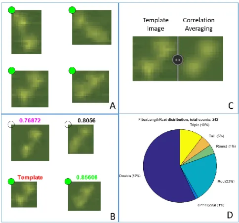
Figure 3.9 Feature Tracking and Enhancement through Cross-Correlation and Correlation Averaging ... 48
Figure 3.10 Processing Periodic Patterns using FFT and Correlation ... 50
Figure 3.11 Particle Detection – Connectivity and Bridging. ... 53
Figure 3.12 Masking Operation ... 56
Figure 3.13. Particle Analysis ... 59
Figure 3.14 The Insufficiencies of Particle Metrics in Describing Shapes ... 60
Figure 3.15. Shape Matching Analysis of Proteins UHRF1 ... 63
Figure 3.16 Particle Classification Module ... 67
Figure 3.17 DNA Tracing and Fiber Analysis ... 72
Figure 3.20 Perimeter Measurement of Contour by Pixel Center ... 83
Figure 3.21 Models for Volume Measurement ... 86
Figure 3.22 Fiber/Skeleton Segmentation... 105
Figure 4.1 Mechanism schematics of DNA Mismatch Repair through the MutSα pathway ... 114
Figure 4.2 Strand Discrimination Signal Searching Mechanism ... 116
Figure 4.3 Mechanism of Repeat Expansion ... 121
Figure 4.4 Experiment Design ... 131
Figure 4.5 A Typical AFM Image of a Protein-DNA Complex and Its Analysis ... 132
Figure 4.6 Selecting Particles for Stoichiometry and Position Analysis ... 132
Figure 4.7 Position Analysis ... 133
Figure 4.8 Volume Distribution of MutSβ Complexes ... 145
Figure 4.9 Stoichiometry of protein complex per DNA ... 147
Figure 4.10 Position Distribution of Protein Complex on DNA ... 148
Figure 4.11 Position Distribution of Protein Complex on (CTG)1 (Single Cut) ... 149
Figure 4.12 DNA Bending by MutSβ ... 150
Figure 4.13 Measuring Kinks on Free DNA ... 152
Figure 4.14 Native DNA Kinks and Their Locations ... 153
Figure 4.15 AFM Images of MutSβ-MutLα-DNA Complexes ... 154
Figure 4.16 Model of Repair Signaling ... 162
Figure A.1 Topographic and DREEM Images of a Polarized Batio3 (BTO) Thin Film ... 163
Figure A.2 Additional DREEM Images of Histone Alone and Nucleosomes ... 164
Figure C.1 Frequency shift on the first overtone with different DC bias ... 180
Figure C.2 DREEM imaging in attractive mode vs. repulsive mode ... 180
Figure C.3 Frequency shift on image contrast ... 182
Figure C.4 Operative Frequency on Image Contrast ... 182
Figure D.1 Welcome Screen of a Typical Module ... 184
Figure D.2 Image Filter Module ... 185
Figure D.3 Action History ... 186
Figure D.4 Macro Builder ... 187
Figure D.5 Batch Processing through Macros ... 188
Figure D.6 Script Editor ... 189
Figure D.7 Image Acquisition... 190
Figure D.8 Image Browser ... 191
Figure D.9 Command Console ... 192
Figure D.10 Shape Matching Analysis of MutSα-DNA Complexes ... 193
Figure D.11 App Manager ... 194
Figure E.1 Restriction map of DNA substrates ... 195
Figure E.2 Position Distribution of Homoduplex from the Double-cut DNA ... 195
Figure E.3 Stoichiometry of Protein Complexes per DNA on Homoduplex from the Double-cut DNA ... 196
Figure F.1 Other Image Artifacts ... 199
Figure G.1 Sub-grouping ... 210
Figure G.2 Super-grouping ... 211
Figure G.3 Hierarchical Ascendant Clustering (HAC) ... 213
Figure G.5 Particle Classification using Artificial Data Set ... 216
Figure G.6 Simulated AFM Image from Classified Particle Images ... 217
Figure G.7 K-means Clustering ... 218
Figure G.8 Cluster Silhouette Plot ... 220
Figure G.9 Comparisons of K-means Clustering using Different Seeds ... 221
Figure G.10 Hierarchical Ascendant Clustering – Flat Cutoff Scheme ... 223
Figure G.11 Hierarchical Ascendant Clustering – Inconsistency Scheme ... 223
Figure G.12 HAC Parameter Optimization ... 224
Figure G.13 Eigenanalysis Parameter Optimization ... 226
Figure G.14 Summary of Classes (w/ Highest Silhouette Means) ... 228
Figure G.15 Summary of Classes (w/ Local Silhouette Maxima) ... 229
Figure H.1 Image Simulator ... 231
Figure H.2 Tip Modeling ... 232
Figure H.3 Tip Geometry Parameterization ... 233
Figure H.4 Tip Apex Simulation ... 233
Figure H.5 Tip Dilation... 234
LIST OF ABBREVIATIONS
AFM Atomic Force Microscopy
CA Clustering Analysis; Correspondence Analysis
DM Dystrophy Myotonic
DREEM Dual Resonance Frequency Electrostatic Force Microscopy EFM Electrostatic Force Microscopy
EM Electron Microscopy
FRDA Friedreich’s Ataxia
FXTAS Fragile X Tremor and Ataxia Syndrome HAC Hierarchical Ascendant Clustering
HD Huntington’s Disease
IM Image Metrics
MMR Mismatch Repair
MRA Multiple Reference Alignment MSA Multivariate Statistical Analysis PCA Principal Component Analysis
ROI Region of Interest
SCA Spinocerebellar Ataxia SNR Signal to Noise Ratio
SL MutSβ-MutLα-DNA Complex
SPIP Scanning Probe Imaging Processor
SXM Scanning X (Force, Probe, etc.) Microscopy
CHAPTER 1. OVERVIEW
Our DNA is subjected to constant damage and metabolic activities during our lifetime. It can be damaged through various exogenous and endogenous factors, or through ‘programmed’ damage during maintenance. It can undergo various structural changes, such as folding into super condensed protein-DNA structures called chromosomes, or unwinding from its double helical structure while undergoing DNA replication, transcription, recombination, and repair [1]. Maintaining the high fidelity of DNA replication during these activities is the corner stone of the central dogma that governs the precise flow of genetic information from DNA to proteins, which is key to our survival.
There are many important cellular mechanisms that govern the high fidelity of DNA replication. DNA mismatch repair (MMR) is one of them [2]. DNA mismatch repair corrects post-replication errors left by DNA replication machinery during DNA replication. Mutations in key DNA mismatch repair genes, first identified in the 1980s, are associated with many cancers, including colon cancer, endometrial cancer, and ovary cancer, collectively called Lynch
Syndrome [3]. It is important to note that DNA mismatch repair proteins also participate in many other cellular processes – most often they assist in positive roles such as signaling for cell
apoptosis, double-strand break repair and homologous recombination [2], but they can also participate in undesirable activities such as promoting a number of trinucleotide repeat (TNR) expansion related neurologic disorders [4], such as Huntington’s Disease (HD).
Atomic Force Microscopy (AFM) is widely used. As a high-resolution, single-molecule imaging technique, AFM has the advantage of directly correlating the conformational structures of protein-DNA complexes to their functions in the context of a repair event [5, 6], while resolving conformational dynamic species that are not observed in crystal structures. However, a limitation of AFM is its inability to resolve the location of the DNA within the multiprotein complex. To tackle this limitation, we developed a new electrostatic force microscopy (EFM) method called DREEM (Dual-Resonance-frequency-Enhanced EFM) that is capable of resolving DNA within protein-DNA complexes (CHAPTER 2).
Another severe limitation to single-molecule AFM studies is the lack of a comprehensive software for high-throughput single-molecule protein-DNA analysis. To reach a statistically relevant conclusion in a single-molecule study, one has to collect and process a large quantity of data, and data analysis is often the bottleneck. To improve the quality and throughput of data analysis, I developed Image Metrics, a new generation image analysis software package (CHAPTER 3). Designed from the ground up, Image Metrics is a comprehensive MATLAB1 -based image analysis package that not only implements features comparable to those found in leading software packages in its category (AFM), but also is specifically designed for easy customization, automation, and streamlining of data analysis. Notably, it features a
single-molecule analysis module that is specifically tailored for high-throughput protein-DNA analysis, the first of its kind to my knowledge. With Image Metrics, users can not only perform all the image processing and analysis in a single package, they can also easily add custom functions, configure their own workflow, and automate laborious routines. I aim to develop Image Metrics as an indispensable tool for AFM image analysis and beyond.
Finally, as a case study, DNA mismatch repair is examined in the context of TNR expansion (CHAPTER 4). AFM is used to visualize directly how MMR proteins interact with heteroduplex DNAs at the initial stages of repair processing. Because a variety of DNA
substrates (both with and without the TNR context) and interaction conditions are involved, a large quantity of data had to be collected for all the conditions combined. The processing and analysis of the collected images of protein-DNA complexes were made possible by utilizing Image Metrics’ high-throughput processing capabilities. Our data analysis shows that when interacting with heteroduplex DNAs without the TNR context, MMR proteins adopt
conformations that are consistent with a repair signaling capable formation; when interacting with heteroduplex DNAs with the TNR context, MMR proteins adopt very different
CHAPTER 2. VISUALIZING THE PATH OF DNA THROUGH PROTEINS USING DREEM IMAGING2
Many cellular functions require the assembly of multiprotein-DNA complexes. A growing area of structural biology aims to characterize these dynamic structures by combining atomic-resolution crystal structures with lower resolution data from techniques that provide distributions of species, such as small angle x-ray scattering, electron microscopy, and atomic force microscopy (AFM). A significant limitation in these combinatorial methods is localization of the DNA within the multiprotein complex. Here, we combine AFM with a new electrostatic force microscopy (EFM) method to develop an exquisitely sensitive Dual-Resonance-frequency-Enhanced EFM (DREEM) capable of resolving DNA within protein-DNA complexes. Imaging of nucleosomes and DNA mismatch repair complexes demonstrates that DREEM can reveal both the path of the DNA wrapping around histones and the path of DNA as it passes through both single proteins and multiprotein complexes.
2 This chapter previously appeared as an article in Molecular Cell. The original citation is as follows - Wu, D., P.
2.1. Introduction
DNA transactions in the cell, such as replication, repair, and transcription, require the assembly of multiple proteins on DNA. Determining the structures of these complexes is essential to understanding their function; however, several factors make characterization of multiprotein-DNA complexes particularly difficult. First, many of the individual proteins are large and contain structured domains connected to one another by intrinsically disordered
regions, making them conformationally diverse. Second, the assembly of the different proteins is not necessarily an ordered process, which results in a heterogeneous population of complexes with different conformations and containing different protein stoichiometries [7]. Finally, the assembly process may occur over long DNA lengths and/or bring distal DNA regions together. An emerging area of structural biology, which is beginning to address this problem, is the combination of high resolution data from crystallography and NMR with lower resolution data from techniques such as small angle x-ray scattering, which provides estimates of the distribution of conformational states [8-11], and electron microscopy (EM) and atomic force microscopy (AFM), which provide images of individual complexes [12-26]. Although these hybrid methods are promising, a significant limitation to the existing lower resolution techniques is their limited capability for resolving the location of the nucleic acids within protein-DNA complexes.
Phosphorus mapping through electron spectroscopic imaging (ESI) has been used to characterize the nucleic acid distribution in transcriptionally active chromatin [27]. In addition, recent
Currently, no microscopy method allows visualization of DNA within flexible and/or large heterogeneous protein-DNA complexes. Because scanning force microscopy methods can provide images of individual complexes and because both proteins and DNA are significantly charged and interactions between proteins and DNA result in charge neutralization, we reasoned that it may be possible to visualize the path of DNA within individual protein-DNA complexes by high-resolution imaging of their electrostatic properties.
Electrostatic force microscopy (EFM) and Kelvin probe force microscopy (KPFM) have been used to image the electrostatic surface potential of a large variety of materials with high spatial resolution and sensitivity [33, 34]. There are several different modes of EFM and KPFM. In many applications, a modulated bias voltage (VDC + VACsin(t)) is applied between the tip and sample. This bias generates an attractive electrostatic force between the tip and the sample,
Fel= -1
2
¶C ¶z DV
2, where
D
V
=
(
V
DC
-D
f
TS)
+
V
ACsin(
w
t
)
and is expressed as the sum of three spectral components [34-36]:𝐹𝐷𝐶 = −
1 2
𝜕𝐶
𝜕𝑧[(Δ𝜙𝑇𝑆− 𝑉𝐷𝐶)
2+𝑉𝐴𝐶 2
2 ] (2. 1)
𝐹𝜔 = 𝜕𝐶
𝜕𝑧(Δ𝜙𝑇𝑆− 𝑉𝐷𝐶)𝑉𝐴𝐶sin(𝜔𝑡) (2. 2)
𝐹2𝜔= 1 4
𝜕𝐶 𝜕𝑧𝑉𝐴𝐶
2 cos(2𝜔𝑡) (2. 3)
where TS and ¶C
measure surface potential, images of the electrostatic properties of the surface are produced by monitoring the amplitude and/or phase of the induced vibration. Dual-frequency single-pass techniques, where the topography and the surface electrical potential are monitored
simultaneously have the highest sensitivity [33, 36-38]. In fact, dual-frequency KPFM has been used to obtain images of DNA [37] and transcription complexes [39]; however, no details about the DNA in the transcription complexes were revealed.
2.2. Design
We adapted and extended the dual frequency single-pass techniques that take advantage of the resonance properties of the cantilever [36-38, 40-42]. To obtain simultaneously both topographic and DREEM images, we mechanically vibrate the cantilever near the fundamental resonance (1), as is done in standard repulsive intermittent contact mode topographic imaging, while applying a static and a modulated bias voltage (VDC and VAC, respectively) to the tip at the first overtone (2) to monitor the surface electrical properties (Figure 2.1) [41]. Instead of using the DC bias to nullify Fw as is done in KPFM, we use an AC bias at 2 to generate a vibration at
2 and apply the DC bias after engaging in repulsive mode to optimize the amplitude at 2 for
electrostatic imaging. We then monitor the vibration amplitude (
A
w2) and phase (
j
w2) as afunction of sample position. Because there is no feedback at the first overtone, the DREEM amplitude and phase signals depend on both the strength of the electrostatic force and force gradient, including the static force gradient (FDC' ) (APPENDIX A) [38, 43-45]. In addition, other forces may contribute to the signal at 2 if they are not canceled by the feedback at the fundamental frequency [38, 43-47]. Generally, the phase image produces higher contrast due to the nonlinear dependence of the phase on the force gradient and energy dissipation (
j
w2
depends on the arcsine of the force gradient and the energy dissipation) [43-45]. For example, studies using dual frequency AFM (with mechanically driven vibration at both frequencies) to image antibodies found that the signal to noise ratio for the phase signal is ~50 times higher than that of the amplitude signal at 2 [47]. Because the force gradient depends on both the
Figure 2.1 Instrumental Design for Simultaneous AFM and DREEM Imaging
The AFM (MFP-3D, Asylum Research) is operated in repulsive oscillating (intermittent contact) mode with the cantilever mechanically vibrated near its resonance frequency (1 = 2𝜋f1) (f1 =~80 kHz, for the cantilever used in
this study) to collect the topographic information. To simultaneously collect the DREEM image, AC and DC biases are applied to a highly doped silicon cantilever (Nanosensors, PPP-FMR, force constant ~2.8 N/m), with the frequency of the AC bias centered on cantilever’s first overtone (2 = 2𝜋f2) (f2 ~500 kHz). An external lock-in
amplifier is used to separate the 2 component from the output signal and compare it with the reference input AC signal to generate the electrostatic amplitude and phase signals. The DC bias is maintained constant and is used to adjust the electrical vibration amplitude to produce optimal contrast in the DREEM images. In the current setup, the
AC and DC biases can be adjusted from 0 V to 20 V and -2.5 V to 2.5 V, respectively. The inset shows the thermal motion of a typical cantilever used in our experiments as a function of the frequency. The frequencies and Q factors
for the fundamental (f1, Q1) and first overtone (f2, Q2) frequencies are shown by each peak.
resonance peak, which is higher at 2 (Q(2) ~500) than at 1 (Q(1) ~170) [49]. Third, the contribution of the electrostatic interaction between the cantilever and the sample to the
electrostatic force is minimized at 2, thereby enhancing spatial resolution in the DREEM image [50]. Fourth, higher eigenmodes provide enhanced phase contrast compared to the fundamental mode of tip oscillation for both AFM and EFM imaging [38, 47, 51].
To determine the optimum voltage for obtaining the highest resolution DREEM
amplitude and phase images, we hold the AC bias constant (usually VAC = 10 to 20 V) and vary the DC bias between +2.5 V and -2.5 V. The optimum DC bias depends on the tip, because the tips can have different extents of oxidation on their surface, which affects TS [52]. Operating in repulsive mode using a cantilever with force constant of ~ 2.8 N/m, the amplitude of vibration at 2 (
A
w2) is ~ 1 nm, which is 30 to 50 times smaller than the mechanical vibration amplitude
(
A
w1) at the fundamental frequency. This
A
w2is sufficiently large to produce high qualityDREEM images and yet small enough compared to
A
w1that no crosstalk from the DREEM to
topographic signals is observed (see below).
A
w2depends not only on the force at 2, but also on
the force gradient,¶F
¶z (i.e., F), because F changes the effective spring constant of the cantilever and shifts its resonance frequency, which in turn, changes
A
w2 [53]. Upon engaging
in repulsive mode, the force gradient due to repulsive atomic interactions (
F
'a) causes the resonance peak to shift to a higher frequency, significantly reducingA
w2. In our experiments,
A
w2decreased by approximately a factor of two upon repulsive engage. During scanning,
F
'
a and Fa is kept constant via feedback on the topographic signal at 1, and therefore, changes in
A
w[
D
A
w2
(
x
,
y
)
] depend primarily on the electrostatic force and force gradient. For small changes inelectrostatic potential and/or capacitance, the frequency shift due to changes in force gradient will dominate
D
A
w2
(
x
,
y
)
, with the electrostatic force making only a small contribution2.3. Results and Discussion
We verified the capabilities of DREEM for detecting surface electrical potential by imaging a BaTiO3 thin film, which can maintain a stable polarization state after being polarized by external electrical field [58-60]. We generated a pattern of very weak negatively and
positively charged areas (~2 electrons/nm2) on a BaTiO3 film (Figure A.1A) [61] and then imaged the sample with AFM and DREEM with different DC and AC biases (e.g., Figure A.1). The topographic image reveals only a rough surface with a large contaminant particle, with no evidence of the charge pattern. In contrast, both the DREEM phase and amplitude signals clearly show the charge pattern, which corresponds accurately to the differently charged areas (Figure A.1B), but show no evidence of the contaminant particle seen in the topographic image. These results demonstrate the capability of DREEM for detecting weak surface charges (< 2
electrons/nm2), with no significant crosstalk between the topographic and DREEM signals. Furthermore, the observation that the contaminant particle does not produce any signal in either the DREEM phase or amplitude images suggests that the dominant force acting at 2 is the electrostatic force.
Visualizing the Path of DNA within Protein-DNA Complexes
amplitude, relative to the mica surface, with proteins producing greater contrast than DNA (Figure 2.2, Figure A.2, and Figure A.3A), as seen in previous EFM studies [37, 39]. The features seen in the DREEM images of free protein mimic those seen in the topographic images (Figure A.2A and Figure A.3A).
Figure 2.2 shows AFM topographic and DREEM images of nucleosomes. In the topographic images, the nucleosomes appear as smooth peaks protruding above the DNA, consistent with previous work [18, 71-77]. In contrast, in the DREEM images, the nucleosomes show regions of decreased intensity within the nucleosomal core particle, and these features are reproducible in multiple scans, scans at different angles, and in trace and retrace images (Figure A.2B). Furthermore, multiple nucleosomes in individual DREEM images display DNA paths at different orientations (Figure A.2). The decreased intensities indicate regions of weaker
the other half (n = 20 out of 41 nucleosomes), we can visualize two DNA stands wrapping around the histone core, where cross-section analysis reveals two distinct peaks corresponding to DNA (Figure 2.2C, and Figure A.2). The distance between the two peaks corresponding to two DNA double strands is 4.2 ± 0.8 nm, which is slightly larger than that seen in the crystal
Figure 2.2 Representative Topographic AFM and DREEM Images of Nucleosomes
(A & B): Topographic (A top, B left), DREEM phase (A middle, B center), and DREEM amplitude (A bottom, B
right) images of nucleosomes showing one DNA wrapping around histones one time. (C): Topographic (left) and DREEM phase (right) images of a nucleosome showing DNA wrapping around nucleosomes twice. Insets show graphs of the height cross-section for the line drawn across the nucleosome in topographic (left) and DREEM phase
(right) images. The two dots on the graph correspond to the positions of the two dots shown on the line across the image, which mark the position of the peaks corresponding to the DNA in the DREEM image. The distance between the two peaks corresponding to the two DNA double strands (dots on graph) is 3.4 nm, which is similar to that seen in the crystal structure (~3 nm) [62]}. Cartoon models of the DNA wrapping around histones are shown on each
DREEM phase image (models are not to scale). The crystal structure of a nucleosome [62]} overlaid on the DREEM phase image is shown in the inset of the phase image in C. The white scale bars are 50 nm. All topographic images are scaled to the same height, and the height scale bar is shown in A. Both the topographic and
DREEM phase images in C are sharper than those in A and B as a result of a sharper AFM tip. All features in the images are seen in both the trace and retrace scans (Figure A.2B). Nucleosomes were reconstituted on a 2743 bp
linear fragment containing 147 bp 601 nucleosome positioning sequence. Unlike the images of nucleosomes, DREEM images of free histones show only smooth “hemispherical shape”, similar to the topographic images
(Figure A.2A). See also Figure A.2.
form multimeric complexes with MutL homologs in the presence of ATP [2, 67-70, 78]. MutS homologs are dimers with DNA binding and ATPase domains, and the DNA binding domains encircle and bend the DNA (Figure 2.3A) [64-66]. In addition, two MutS dimers can associate to form DNA loops [6, 79, 80]. Furthermore, in the presence of ATP, MutS homologs form a mobile clamp after mismatch recognition that can move away from the mismatch which allows multiple proteins to load onto DNA containing a single mismatch [78, 81-83]. Topographic AFM images of T. aquaticus (Taq) MutS bound to a GT mismatch (Figure 2.3B) and two MutS
dimers forming a DNA loop between the mismatch and a DNA end (Figure 2.3C) show the typical smooth peaks on the DNA corresponding to Taq MutS [5, 6]. In contrast, in the DREEM images (Figure 2.3) the “peaks” corresponding to the position of MutS show regions of
other images (not shown) suggests that the contrast between the DNA and protein in the DREEM images depends on how close the protein-DNA interaction site is to the tip. If the DNA is
Figure 2.3 Topographic AFM and DREEM Images of Mismatch Repair Complexes on 2 kbp DNA Containing a GT Mismatch
(A) Space-filling model of the crystal structure of Taq MutS (generated from PDB 1EWQ). Subunits A and B and the
DNA are colored blue, gold, and cyan, respectively. MutS bends the DNA by ~ 60° as it passes through the DNA binding channel. (B) AFM topographic (left) and DREEM phase (center) and amplitude (right) images of a Taq MutS-DNA mismatch complex. Model of the complex is shown overlaid onto the AFM images and next to the phase
images. (C) AFM topographic (left) and DREEM phase (right) images of two MutS dimers forming a loop in the DNA between the location of the mismatch (375 bp from one end) and DNA end. Model of the complex is shown overlaid onto the AFM images and next to the phase images. The model is based on the volume of the complex in the
topographic image (consistent with two dimers), the location of the DNA in the DREEM image, as well as the crystal structure and the location of the tetramerization (two MutS dimers) interface [85, 86]}. A topographic surface plot of this image is shown in Figure 2.1. (D) AFM topographic (left: surface plot) and DREEM phase (middle: surface plot; right: top view) images of a large MutS-MutL-DNA complex containing ~10 proteins. The path of the DNA is identified as the regions with highest reduction of the magnitude of DREEM signals compared to protein alone and traced in the inset in blue. Interestingly, the DNA appears to be sharply bent after entering the
Limitations
Other than the requirement that the samples must be deposited on a surface to be imaged, which is common to all scanning probe microscopies, the primary limitation of DREEM relates to the use of highly-doped silicon cantilevers. Although doped diamond-coated cantilevers (tip radius ~100 nm) and metal-coated cantilevers (tip radius ~30 nm) are typical choices for EFM imaging [87], they are not sufficiently sharp to produce high-resolution images. Highly-doped silicon cantilevers are sharp (5-8 nm) and sufficiently conductive for high-resolution topographic and DREEM imaging; however, the quality of the DREEM image appears to depend on the oxidation layers on the surface. The oxidation layer on the silicon cantilevers requires that the DC and AC biases be optimized for each cantilever. These differences in oxidation layers prevent quantitative comparison of the magnitudes of the DREEM signals collected with different tips, or the same tip after collecting a series of images. In addition, ~30% of prepared conductive silicon cantilevers do not generate sufficient contrast between the protein and DNA to allow us discern paths of DNA in protein-DNA complexes in DREEM images. Argon plasma cleaning of the cantilevers prior to use appears to improve their quality for DREEM imaging. Finally, the quality of the DREEM images degrades during imaging faster than that of the topographic images. Typically, ~10 to 12 high-quality DREEM images can be obtained from a single AFM tip.
identified by the repetitive features in different molecules from the same image and by scanning at various angles.
A final limitation of DREEM is that it is currently limited to imaging in air. At present, we have not been able to identify operating parameters that allow contrast in aqueous
environment. A few studies demonstrate EFM imaging of solid materials at low ionic strength using lift mode [88, 89]; however, the resolution and detection limit in these images appears low. It is likely that the electrostatic double layer significantly damps the DREEM signals from proteins and DNA in electrolyte solutions.
Conclusions
In summary, while the paths of DNA are hidden in protein complexes in traditional microscopy imaging techniques, such as AFM and EM imaging, DREEM allows the
visualization of the conformation of DNA within individual protein-DNA complexes. In addition to the studies presented here, DREEM also has been utilized to visualize DNA conformations within telomere binding proteins (Benarroch-Popivker et al., 2016; unpublished results, Kaur, Wu, Lin, Countryman, Bradford, Erie, Riehn, Ospresko, Wang). Taken together, the capability of DREEM to detect very small changes in electrostatic force gradient with high resolution makes it a powerful tool for characterizing the structure of protein-DNA complexes at the single-molecule level. It will be especially useful for characterizing protein-DNA complexes with long length scales and those that result in heterogeneous populations of proteins on the DNA.
orientations of proteins in multiprotein assemblies on DNA, as demonstrated by our ability to dock the crystal structure of the nucleosome into a subset of the images. In addition, DREEM allows the path of DNA to be resolved in large heterogeneous multi-protein-DNA complexes. It also will be applicable for characterizing the electrostatic properties of other biological
specimens, such as viruses and membranes, as well as non-biological samples. With sharper tips and further refinement of the technique, it is highly likely that the resolution can be further increased in the future. Finally, with the addition of only two components (a function generator and a lock-in amplifier, Figure 2.1), DREEM can be implemented on many of the commercially available AFMs, making it readily available to many labs.
Experimental Procedures
Instrument design
Our experimental setup for simultaneous AFM and DREEM is described in Figure 2.1. In our setup, we apply an AC bias at the first overtone (2) and monitor the vibration amplitude (
A
w2) and phase (
j
w2) as a function of position, while simultaneously collecting thetopographic image at the fundamental frequency (1).
The detailed methods for conductive cantilever preparation, substrate grounding, selection of imaging conditions, sample preparation, deposition, and analysis are described in Appendix A.III.
Supplementary Information
Supplementary Information, which includes the theoretical basis of DREEM,
Author Contributions
D.W. and D.A.E. invented the DREEM method. KCB prepared human mismatch repair protein-DNA samples. D.W., P.K., Z.L., H.W., and D.A.E. designed and conducted
experiments, analyzed data, and wrote the manuscript.
Acknowledgements
CHAPTER 3. IMAGE METRICS, A NEXT-GEN AFM IMAGE ANALYSIS SOFTWARE One of the biggest hurdles in single-molecule AFM studies is the lack of comprehensive software package that allows for high-throughput analysis. In fact, data analysis is often the bottleneck in single-molecule studies. To tackle this issue, I developed Image Metrics, a full-featured MATLAB3-based AFM image analysis software package. Relying on MATLAB’s enormous scientific library, Image Metrics is able to blend powerful features and flexibility into a user-friendly interface, and enable users to perform high-throughput multi-faceted image analysis. In particular, Image Metrics features unique modules for single-molecule analysis and shape analysis such as particle classification that are not available in other AFM software. With Image Metrics, single-molecule AFM analysis is streamlined - image correction, measurement, and analysis are all processed in a single software package, and users can easily program user functions, customize workflows, and automate laborious routines. The software is designed to be the next generation research tool for AFM and other imaging fields.
3.1. Introduction
In single-molecule AFM studies, usually a large amount of data has to be collected and processed to reach a statistically relevant conclusion. Increasing the quantity of data should improve the quality of data analysis; however, the time required for image analysis is a major limiting factor in increasing the sample. Consequently, a software package capable of analyzing single-molecule data in high throughput is sorely needed.
Despite the many software packages available ([90], Ref. Appendix C), none of them are tailored for single-molecule AFM studies. Table 3.1 (white rows) gives an overview on major software in the market. While particle analysis exists as a stock feature for many programs (Table 3.1 Particle Analysis) [91, 92], the particle metrics (Table 3.3) analyzed are too generalized to describe complex conformations such as those of protein-DNA complexes. To analyze such conformations, users have to zoom manually in to the region of interest and
perform a variety of measurements, such as DNA profile and DNA bend angle, which is a highly repetitive and time-consuming task. On top of that, none of the software offers vertically
integrated capabilities to manage data recordings for such analysis4. While certain workflows can be automated with preset functions in some programs (Table 3.1 Macros), they are often basic or difficult to use. Few software is comprehensive enough to complete all the image processing and analyses required for single-molecule AFM studies in a single package, and the technicality of programming custom functions is too complicated for users without a computer science
4 The recording and management of measurement data on existing software is deferred to the users – often requiring
background5. Many software packages are also poorly maintained, documented, or interfaced6. Overall, none of the software is capable of performing single-molecule analysis in
high-throughput. Their shortcomings add significant time overhead and costs to users’ workflow, which typically involves three or more programs, and present a huge challenge to single-molecule AFM studies.
To tackle this problem, I developed Image Metrics (Table 3.1 grey row), a professional image processing and analysis software. Image Metrics is written in MATLAB from the ground up and incorporates innovative and comprehensive features into a user-friendly, well
documented interface. It is specifically designed to allow for high-throughput single-molecule analysis, and is compiled as a royalty free standalone application that runs across all major platforms. With the advent of Image Metrics, single-molecule AFM analysis is streamlined: image import, calibration, processing, analysis, and results output can be carried out all within the same program. Notably, Image Metrics features advanced fiber analysis and shape analysis that are unique to the field of single-molecule AFM studies such as the study of protein-DNA conformations and the classifications of molecular conformations. Image Metrics also provides unique flexibility that allows users to customize and automate workflows without advanced coding skills and to write custom functions through the built-in scripting interface. Collectively, these strengths provide researchers a cost-effective and incentive application platform to port
5 For example, writing extensions for these programs requires advanced knowledge of general purpose programming
language (C, C++, Python, Java, etc. Table 3.1Extensions), which requires a lot of heavy-lifting on the users’ end to take care of many general aspects of computing such as memory management, complicated syntax, and
integration of external libraries, etc.
6 For example, many software packages (Asylum Research, Nanoscope analysis, ImageJ, WSxM, etc.) are not
their own applications, which could open up Image Metrics to fields far beyond its original scope.
Software Image Formats Platforms Image Processing Particle Analysis Fiber Analysis Bend Angle 1 Asylum
Research
Asylum Research format
Windows,
macOS Yes Yes Yes No
2 Gwyddion Various Multiple Yes Yes No No
3 Image
Metrics Various Multiple Yes Yes Yes Yes
4 ImageJ Nanoscope format Multiple Yes Yes Yes No
5 ImageSXM Various macOS Yes Yes No No
6 Nanoscope
Analysis Nanoscope format Windows Yes Yes No No
7 SPIP Various Windows Yes Yes Yes Yes
8 WSxM Various Windows Yes No No No
Macros Extensions Source License Ref. URL
1 Yes Igor Pro Available7 Free http://support.asylumresearch.com
2 Yes C, Python Open GNU [92] http://gwyddion.net
3 Yes MATLAB Available8 Free http://im.zimengli.com
4 Yes Java Open BSD [93,
94] http://imagej.net
5 Yes No Closed Free [95] https://www.liverpool.ac.uk/~sdb/ImageSXM
6 Yes No Closed Free http://nanoscaleworld.bruker-axs.com/
7 Yes C++, C# Closed ~$10k [96] http://imagemet.com
8 Yes No Closed Free [97] http://www.wsxmsolutions.com
Table 3.1 Overview of major AFM Software for Single-Molecule AFM Study
Other AFM software includes SFMetrics [98], GXSM [99], DockAFM [100], OpenFovea [101], FRAME [102], DeStripe [103], DNA Trace [104], FiberApp [105], and various manufacture software from JPK instrument, Bruker, etc. Image Formats: ‘Various’ means support for images from multiple AFM vendors. Platform: ‘Multiple’
means support for Windows, macOS, and Linux. Image Processing: standard image corrections (Section 3.4).
Particle Analysis: batch analysis of particle metrics (Section 3.5.2A). Fiber Analysis: measuring profile and length
of fiber such as DNA (Section 3.5.3B). Bend Angle: measuring DNA bend angle and curvatures (Section 3.5.3D).
Macros: scripts that automate program functions (Section 3.6), also known as global analysis or batch analysis. Extensions: external programs that acts natively and implement additional functions (Section 3.6). Also known as
plugins or modules. Source: Open source licenses such as GNU and BSD allow for free modification, contribution, and distribution of code. Source available software limits the modification and distribution of code in some way. Closed source software is also referred as proprietary software. License: GNU and BSD are open and free licenses.
SPIP pricing is quoted as the full/premium-feature installation price per seat.
7 Users can modify, but not contribute to the code.
Due to the scope of this study, I will mostly discuss applications of Image Metrics that are relevant to single-molecule AFM studies, and briefly mention other applications where applicable. Details of all its functions and instructions can be seen on its website
3.2. Interface
Image Metrics is designed to maximize the accessibility, flexibility, and availability to users of all major desktop platforms. It runs on the latest Windows, macOS, and Linux
distributions. It consists of different modules (called ‘apps’) united under a single application launcher (Figure 3.1). The design language of a typical module consists of ribbons9, toolbars, search bar, workspace, and a status bar (Figure 3.2).
A welcome screen serves as both recent file lists and tutorials on most modules (Figure D.1). Tutorials are composed of step-by-step guides, demos (usually images), online videos, and online instructions. Functions are designed to be easily accessible throughout the program. Users can place their most often used functions in the mini toolbar or in the quick access bar, and keyboard shortcuts can be assigned to most functions. Accessibility-wise, the software is DPI10 aware and fits into most monitor resolutions, sizes, and dimensions. Font and window size can be adjusted without compromising software usability. Most functions will also remember their last known parameters, so user preference will be saved upon exiting and reloaded upon relaunching.
9 Also called Toolstrips in software such as MATLAB
10 Dots per inch or DPI is a measure of display scaling factor. Larger DPI means larger, more visible interface
Figure 3.1 Image Metrics Application Launcher
The Application Launcher is the central place to manage and launch Image Metrics apps. The apps are arranged by groups based on their categories. Apps can be added to favorite as shortcuts. Users have the ability to load custom
Figure 3.2 Image Metrics User Interface
Application modules are launched through the Application Launcher. Featured in the image is the Region Inspector module. Toolbar and Ribbon provides access to major application functions. The search bar allows users to find a
function by its description or name or used to search for help. Workspace is the main working area of an application module. Frequently accessed functions can be placed on the mini toolbar and/or the quick access bar. The mini toolbar is context sensitive, but can be pinned on top of the workspace. The status bar can display helpful
3.3. Basic Operations
A. Image I/O and Calibration
Similar to many programs (Table 3.1 Image Formats), Image Metrics supports multiple image formats. Currently, Image Metrics supports direct import of raw AFM data from several manufactures (Asylum Research, Veeco/Bruker, JPK Instrument, etc.)11 in addition to
conventional image and video formats12. Users can also set up custom imports if file I/O codes are provided, of which many can be found on MATLAB File Exchange or on third-party websites. Image Metrics also features an Image Acquisition module (Figure D.7) and Image Simulator module (Figure H.1) for acquiring images from external and synthetic sources. The Image Acquisition module relies on MATLAB’s Image Acquisition Toolbox, which supports many microscope hardware13. While not directly supporting AFM image acquisition, it is possible to communicate with external AFM hardware if a software interface is provided by the AFM manufacturer14. The Image Simulator module provides simulation of AFM images using 3D models that can either be parameterized shapes or 3D models from external files such as those from the protein data bank (PDB). The module also lets users perform tip modeling and apply tip dilation to images using methods described in previously published papers [106, 107]. Interested readers can find more details in APPENDIX H. To save processed or analyzed data,
11 Manufacture file I/O is achieved via several submissions in MATLAB File Exchange, see Section 3.8 for license and copyright information.
12 Formats that are natively supported by MATLAB.
13 Currently, most hardware packages are based on camera systems. AFM vendors traditionally use proprietary
software to control their system. However, the potential to open such access to users is there.
14 For example, in Asylum Research software, many AFM commands can be accessed at the command line and
users can save them into an Image Metrics specific file (.im) that also can be imported into MATLAB as a MAT file15 for further processing in MATLAB.
After images are imported, they can be automatically calibrated to proper units if
calibration data are contained in image files. Otherwise, images can be calibrated manually in the four dimensions (x, y, z, t) in user defined units. The wide range of image formats supported and the flexibility to use custom units allow Image Metrics to adapt to a wide range of imaging applications, ranging from microscopic (molecular and cellular biology, material sciences) to macroscopic (geography and astronomy), from still images (e.g. static AFM imaging) to dynamic images (e.g. high-speed or time-lapsed AFM imaging, fluorescence microscopy, etc.).
B. Image Navigation
In Image Metrics, images are treated as containers. Each image can contain one or more layers (named data channels in Image Metrics). For example, an AFM image can contain multiple channels (height, amplitude, phase, etc.); a color image contains three color channels (RGB); a dynamic image (video) uses its frames as channels. Similar to other AFM programs, an
Image Browser module (Figure D.8) is incorporated in Image Metrics to help navigate the images and different image layers more easily. From there, users can remove images, open new images, and duplicate images. Image Metrics also features an Image Viewer module (similar to SPIP’s inspection window) so that users can open the same image, or different images, in different windows for close-up inspections, cross comparisons, and/or synchronized views. Imported images can be edited (e.g. resized, cropped, corrected) and exported as individual images or videos for publication or processing in other programs.
C. Image Visualization
AFM images are intensity images. Similar to other AFM programs, they are visualized via pseudo-color or false colormap [92, 97, 108]. Image Metrics offers a variety of color maps to help image visualization. Users can change the contrast of a color map or customize the color map with easy slider-based adjustment tools. The color map can also be loaded from or saved to external files for easy sharing and backup, and many professional colormaps and colormap utilities16 from various fields of study can be downloaded from MATLAB file exchange. To change the data range to which the colormap applies, users can either manually enter the data range or use the program’s built-in function to determine the data range based on region of interest, which can be either the whole image or a custom drawn region (Figure 3.3A). Users can also make the intensity distribution plot, where they can place range markers to change the lower and upper end of the color map interactively (Figure 3.3B). Many AFM programs interpolate data when zoomed in (e.g. Asylum Research). Although Image Metrics does not interpolate data by default when zoomed in (Figure 3.3C), it can be done if the user chooses (Figure 3.3E). As with many AFM programs, 3D surface plots can be rendered to visualize the topographic
information. Apart from the conventional 3D operations, the program also features a very useful image overlay function that allows another image channel (usually represents another AFM signal channel such as force, phase, voltage etc.) to be overlaid on top of the topography as a color layer. Contour plots can also be overlaid to visualize easily the change of intensities in regions of interest (Figure 3.3F). The image and contour overlay function is only available in the commercial software SPIP besides Image Metrics.
Figure 3.3. Image Visualization
A. Image to be visualized (height channel). In Image Metrics, users can draw an area (blue box) that automatically
scales the colormap to the data range within that area. B. Intensity distribution plot. Users can place two marker bars to adjust the upper and lower limit of the current colormap and interactively affect the image appearance in A.
C. DREEM phase channel (see DREEM imaging on CHAPTER 3) of the same image as A. D. Zoomed-in view of
3.4. Image Processing
Similar to other types of imaging techniques, AFM imaging comes with image artifacts that usually require correction before the images can be analyzed. AFM image artifacts typically derive from factors that impact the probe-surface interaction, such as: (1) tip degradation and contamination; (2) excessive or lack of image force that leads to improper tracking of the surface; (3) factors that impact the performance of the AFM scanner and feedback system, such as environmental noise, piezo drifting, and improper gain settings on the feedback system. Although many artifacts can be corrected to various degrees, not all the corrections make for easier or better analysis. Some of them require complex calculations and calibrations and may introduce new artifacts due to over-correction, therefore, the decision to correct various artifacts must be determined at the level of individual studies. In Image Metrics, the Image Processor
module (Figure D.1) is specifically designed to process and correct images. Here, I discuss the most relevant features in Image Metrics to correct some of these image artifacts. For processing other typical image artifacts, see APPENDIX F.
3.4.1. Surface Correction
features, and in the worst scenario, transformation of surface features (Figure 3.7B red box). The amount of drifting is directly impacted by scan speed, with faster scanning resulting in lower drifting. (b) Non-linearity of piezo response along the scan line ([110], [90] Ref. Section 2.2.1): Piezo typically suffers from non-linear response17 with increasing scan size, especially when the scan size approaches the scanner limit, resulting in ‘scan bow’ effect (Figure 3.7C), and from hysteresis effect18 between tracing and retracing of the surface, resulting in differential heights between the trace and the retrace images. (c) Scanning over an uneven or tilted surface ([90] Ref. Section 5.1.1): Even for a flat even surface like freshly peeled mica, tilt could still occur if the mica is not glued evenly to its mounting substrate, the substrate is unevenly mounted, or the scanner is not leveled parallel to the platform upon imaging, resulting in an uneven image (Figure 3.4).
These changing heights along the line or from line to line, if not normalized, results in an uneven image (Figure 3.4, Figure 3.7C) that otherwise should be an even flat surface like the mica used in single-molecule protein-DNA AFM studies. Even if the surface is inherently uneven, it may still require normalization for analyzing some surface features, especially if height-based calculation (e.g. masking, volume calculation, etc., more on that later19) is needed. Without correction, the unevenness offsets surface features differentially by their local surface heights and presents a challenge to measure or process anything that is height related accurately.
17 Piezo linearity is indicated by a linear curve of applied voltage vs. piezo displacement.
18 Hysteresis is a common effect in ferromagnetic, ferroelectric, and piezoelectric materials. It’s indicated by the
non-linearity of the material response when upping and lowering the applied voltage within the range of two set voltages.
Figure 3.4 AFM Scan Line Image Artifact
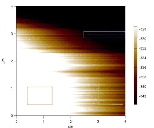
A typical, unprocessed AFM image is shown. Three types of scan line artifacts may arise. Green box: Uneven heights along the slow scan axis (y axis) originate from Z-piezo drifting. Orange box: Uneven heights compared to
green box along the same scan lines. This artifact could be originated from multiple causes: (a) non-linearity of piezo response along the scan line. (b) Z-piezo drift (thermal or mechanical). (c) uneven or tilted surface. Blue box:
line artifact along the scan line when tip stumbles upon a tall feature (resulting in spikes) or sucks in a low feature (resulting in dark stripes).
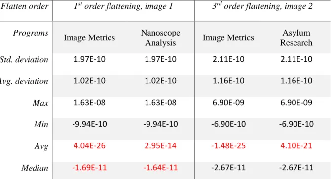
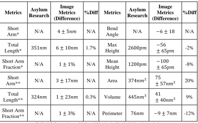
individual image are usually needed to normalize the surface accurately. To validate the
algorithm used in Image Metrics, a comparison between Image Metrics and other AFM software is shown in Table 3.2. The differences (Table 3.2, red highlights) are orders of magnitudes below the pixel variations of a flat mica surface (Table 3.2, std. deviation and avg. deviation), and are likely resulting from rounding errors in the underlying numerical packages used by the different programs. In addition, surface features, including high features such as protein-DNA complex or low features such as surface wells or pores, can be excluded or masked from the curve fitting using a height-based threshold ([90] Ref. Section 5.1.1) or clustering methods [108] (Figure 3.7D), thereby eliminating outliers that could derail the surface normalization. Such operation is often called masked flattening (Asylum Research software), or flattening with thresholding (Nanoscope Analysis). Image Metrics also provides a novel Gaussian-based algorithm that automatically calculates the optimal surface threshold used to mask the features without masking too much surface (Figure 3.6). It should be noted that the line-wise correction will not correct a real warped or slanted surface, but a flattened surface may still be desirable for easier measurement of relative heights. In those scenarios, a planefit (two-dimensional
Figure 3.5 Detrend Operation
A section profile along the scan line is shown on the left (blue), which can be fit into a polynomial curve (red curve, here the 3rd order polynomial fit is used). Subtracting the polynomial curve from the section profile results in a flat,
normalized base line in the profile (right). In this example, thresholding is used to exclude the outliers (spikes) from polynomial fitting.
Flatten order 1st order flattening, image 1 3rd order flattening, image 2
Programs
Image Metrics Nanoscope
Analysis Image Metrics
Asylum Research
Std. deviation 1.97E-10 1.97E-10 2.11E-10 2.11E-10
Avg. deviation 1.02E-10 1.02E-10 1.16E-10 1.16E-10
Max 1.63E-08 1.63E-08 6.90E-09 6.90E-09
Min -9.94E-10 -9.94E-10 -6.90E-10 -6.90E-10
Avg 4.04E-26 2.95E-14 -1.48E-25 4.10E-21
Median -1.69E-11 -1.64E-11 -2.67E-11 -2.67E-11
Table 3.2 Comparison of Image Flattening Results between Image Metrics and other AFM software.
Examples of two different orders of flattening (1st and 3rd) in Image Metrics compared to two different AFM
software. A different image is used for the two comparisons because the two AFM software do not open the same image format. The samples imaged are composed of mica surface with protein-DNA sample (e.g. image 1 can be seen in Figure 3.7A-B), and therefore are relatively flat (with surface standard deviation of around 200pm). The difference resulting from the flattening procedures used by different AFM programs are highlighted in red. As can be seen in the table, the difference is orders of magnitudes below the surface’s standard deviation, and because the surface is relatively flat, the difference can be seen as negligible, and likely results from rounding errors used by the
Figure 3.6 Auto Threshold by Gaussian Method
A. Usually when user chooses a height threshold, it is often subjective and not accurate, resulting in fluctuations in
the excess of how much surface is masked (with consequence of affecting the accuracy of the masks). B. The threshold is manually chosen by looking at the intensity distribution. C. Using the built-in Gaussian method, threshold is chosen accurately by the computer, resulting in less subjectively and enhanced reproducibility and accuracy. D. The way the Gaussian method works is to fit the intensity peak to a Gaussian curve, and an offset to the center of the Gaussian is used to determine the surface threshold. The offset is predefined as a percentage drop from the peak. Because the breadth of the peak is indicative of the intensity of the background noise, this method adjusts
the offset proportionally to the breath of the peak, and therefore is background noise independent and is able to achieve high accuracy in masking the features without masking the surface.
low or too high such that the feedback system fails to properly track the surface ([110], [90] Ref. Section 4.2.3). The abnormality in surface tracking could result in elongated feature along the scan line, or a sharp scan line (also called stripe, spike, or shot noise) that stands far above or below normal scanning height (Figure 3.8A red boxes, Figure 3.4 blue box, Figure 3.7B white box), or in the case of excessively high gain settings, periodic recurrence of up and down patterns known as ringing noise. Generally, the information is lost or distorted, and features affected by the artifacts should be discarded, but scan line noise can usually be partially negated by filling with neighboring pixels, in which case a threshold-gated median filter is often used (Figure 3.8D) [96, 108]. The median filter20 defines a pixel as an outlier if its value surpasses a certain threshold beyond the average value of it and its nearby neighbors (also called the kernel window or kernel size, which can be set by the users). In Image Metrics, the threshold is defined as a percentile of the standard deviation of the kernel window. It can also be defined as a
percentage of worst outliers to be modified (SPIP) [96]. The outlier pixel, once determined, is then replaced by the median value of the filter kernel. Locating and removing the stripe artifact can be manual (e.g. erase line function in Asylum Research, Figure 3.8F) or automatic (e.g.
remove thin bright line functionin SPIP, Figure 3.8E). The automatic procedure used by SPIP applies the median filter across the whole image, which could incorrectly filter information that is not shot noise (such as a tall protein) (Figure 3.8D). To prevent such situations, it is preferable to apply the filter only on the line or line segment where the shot noise is. In a previous
published algorithm [108], the line is located by comparing the average of each line to identify the outlier as the aberrant line with the stripe. In Image Metrics, in addition to filtering the whole
20 There are several kernel filters available in Image Metrics, including median, gaussian, wiener, standard deviation,
line by outlier, the line can further be segmented by filtering the line by area or by an outlier threshold21 (Figure 3.8E). For example, in the case of a stripe line segment, its area is always larger than isolated “noise” from misinterpreted tall proteins. The outlier threshold further singles out the true noise from randomly misinterpreted “noise” by filtering out data with only small variations. In Image Metrics, all the filter operations are handled in the Image Filters
module (Figure D.2), where filter parameters can be adjusted interactively to preview results in real time, and they be saved as custom filtering profiles for batch processing (Section 3.6).
Figure 3.7. Correcting Line-wise Image Artifact
A. Raw AFM trace image (i.e. scan direction is from left to right) of a protein-DNA sample deposited on mica.
Notice the variation in heights among different scan lines along the y axis. B. 1st order flattening of the raw image.
White box – scan line noise resulted from tip stumbling over a protein complex. Notice that a black line occurs along the same scan line due to overcorrection by the flattening procedure. Red box – features distortion (elongation diagonally) caused by piezo drifting and/or residual movement of the piezo. C. Image in B is masked by
a height-based threshold to reveal the shape of the measured surface. In this case, the surface is warped in the middle, resulting from a parabolic tracing pattern along the scan line. D. A new threshold is chosen to mask only the protein and DNA molecules, thereby excluding them from the surface normalization. E. A 2nd order flattening is
Figure 3.8 Line Removal Algorithms Compared
(A) Raw image. Shot noise is highlighted in red boxes. (B) Automatic line removal through Image Metrics. (C) Manual line removal through Asylum Research software. (D) The difference image in binary (black and white image) generated from Image Metrics’ or SPIP’s median filter procedure. The difference image is obtained by subtracting the raw image by the modified image, followed by a logical operation that converts modified pixels to 1
(bright color) and unmodified pixels to 0 (dark color). As seen in the image, the modified pixels include both the stripe noise and non-noise information. (E) The difference image in binary generated after applying an outlier threshold and/or an area threshold. The outlier threshold makes sure only data (after applying the initial median filter in D) that have big changes (i.e. above the threshold value) are modified. The area threshold makes sure the noise is line in nature and not random isolated noise (as a line stripe contains more pixels than isolated pixels). As seen in the image, only the line segments representing the stripe noise is removed. (F) The difference image in binary generated from Asylum Research software’s manual line removal procedure. The manual removal erases the whole line, and therefore pixels along the whole line are modified. This result could have undesirable consequences