DOI:10.1051/0004-6361/201630323
c
ESO 2018
Astronomy
&
Astrophysics
A method of immediate detection of objects with a near-zero
apparent motion in series of CCD-frames
V. E. Savanevych
1,2, S. V. Khlamov
2, I. B. Vavilova
3, A. B. Briukhovetskyi
1, A. V. Pohorelov
4, D. E. Mkrtichian
5,
V. I. Kudak
2,6, L. K. Pakuliak
3, E. N. Dikov
7, R. G. Melnik
1, V. P. Vlasenko
1, and D. E. Reichart
81 Western Radio Technical Surveillance Center, State Space Agency of Ukraine, Kosmonavtiv Street, 89600 Mukachevo, Ukraine e-mail:[email protected]
2 Uzhhorod National University, Laboratory of space research, 2a Daleka Street, 88000 Uzhhorod, Ukraine e-mail:[email protected]
3 Main Astronomical Observatory of the NAS of Ukraine, 27 Akademika Zabolotnogo Street, 03143 Kyiv, Ukraine 4 Kharkiv National University of Radio Electronics, 14 Nauki Avenue, 61166 Kharkiv, Ukraine
5 National Astronomical Research Institute of Thailand, 260 Moo 4, T. Donkaew, A. Maerim, 50180 Chiangmai, Thailand 6 Institute of Physics, Faculty of Natural Sciences, University of P. J. Safarik, Park Angelinum 9, 04001 Kosice, Slovakia
7 Scientific Research, Design and Technology Institute of Micrographs, 1/60 Akademika Pidgornogo Street, 61046 Kharkiv, Ukraine 8 Department of Physics and Astronomy, University of North Carolina at Chapel Hill, Chapel Hill NC-27599, North Carolina, USA Received 22 December 2016/Accepted 25 September 2017
ABSTRACT
The paper deals with a computational method for detection of the solar system minor bodies (SSOs), whose inter-frame shifts in series of CCD-frames during the observation are commensurate with the errors in measuring their positions. These objects have velocities of apparent motion between CCD-frames not exceeding three rms errors (3σ) of measurements of their positions. About 15% of objects have a near-zero apparent motion in CCD-frames, including the objects beyond the Jupiter’s orbit as well as the asteroids heading straight to the Earth. The proposed method for detection of the object’s near-zero apparent motion in series of CCD-frames is based on the Fisher f-criterion instead of using the traditional decision rules that are based on the maximum likelihood criterion. We analyzed the quality indicators of detection of the object’s near-zero apparent motion applying statistical and in situ modeling techniques in terms of the conditional probability of the true detection of objects with a near-zero apparent motion. The efficiency of method being implemented as a plugin for the Collection Light Technology (CoLiTec) software for automated asteroids and comets detection has been demonstrated. Among the objects discovered with this plugin, there was the sungrazing comet C/2012 S1 (ISON). Within 26 min of the observation, the comet’s image has been moved by three pixels in a series of four CCD-frames (the velocity of its apparent motion at the moment of discovery was equal to 0.8 pixels per CCD-frame; the image size on the frame was about five pixels). Next verification in observations of asteroids with a near-zero apparent motion conducted with small telescopes has confirmed an efficiency of the method even in bad conditions (strong backlight from the full Moon). So, we recommend applying the proposed method for series of observations with four or more frames.
Key words. methods: numerical – methods: data analysis – techniques: image processing – minor planets, asteroids: general – comets: general – comets: individual: ISON
1. Introduction
Different types of objects are detected in series of CCD-frames during observations: solar system minor bodies (SSOs); stars and large-scale diffuse sources (non-SSOs); charge transfer tails from bright stars, bright streaks from satellites, and noise sources amongst others. The difference between the detected SSOs and non-SSOs is that the non-SSOs have a zero velocity apparent motion on a set of frames, while the SSOs have a non-zero one. Wherein, a rapid detection of the objects with a near-zero veloc-ity apparent motion both from the main belt of asteroids and be-yond the Jupiter’s orbit is very important for the asteroid-comet hazard problem as well as for the earliest recording new SSOs.
Over the past few decades, several powerful software tools and methods had been developed, allowing discovery and cataloging of thousands of SSOs (asteroids, comets, trans-Neptunians, Centaurs, etc.). First of all, it was the Lincoln Near-Earth Asteroid Research (LINEAR) project (Stokes 1998), which outperformed all asteroid search programs acted
until 1998. This project brought the number of discovered SSOs to over 230 000, including 2423 near-Earth objects (NEOs) and 279 comets (Stokes 2000). The second biggest asteroid sur-vey, the Catalina Sky Survey (2016), started in 2005 as a search program for any potentially hazardous minor planets and al-lowed to discover more than 6500 NEOs. The same program in the southern hemisphere, the Siding Spring Survey (SSS), was closed in 2013.
(Shucker 2008). Another algorithm, the interacting multiple model (IMM), was introduced as a modification of matched fil-ter and provided a new structure for effective management of multiple filter models, while the selected parameters must be considered for the IMM optimizing (Genovese 2001).
The Panoramic Survey Telescope and Rapid Response System (Pan-STARRS) for surveying the sky for moving objects on a continual basis was designed as an array of four telescopes. The first telescope, PS1, is in a full operation since 2010 and is able to observe objects down to 22.5mapparent magnitude. With the help of PS1 more than 2860 NEOs and many comets have al-ready been discovered (seeHsieh et al. 2013). PS1 uses the Mov-ing Object Pipeline System, MOPS (Heasley et al. 2007), which includes some methods and techniques for searching for the ex-tremely faint and distant Sedna-like objects (Jedicke et al. 2009), such as for example the modified intra-nightly linking algorithm, which includes a partial Hough transform method for quickly identifying of the multiple detections and post-processing step for intra-nightly linking (see, Parker et al. 2009; Myers et al. 2008).
These methods were successfully tested for simulations of processing the moving objects with MOPS on the Pan-STARRS and the Large Synoptic Survey Telescope, LSST (Barnard et al. 2006), the latter will be provided by the same pipeline system as on the Pan-STARRS (Myers et al. 2008). It is important that PS1 is highly effective for discovering objects that could actually impact the Earth next 100 years (Jedicke et al. 2009) and was complemented with the infrared data of the former WISE orbital telescope (Dailey et al. 2010).
In 2009, the authors of this paper developed the CoLiTec (Collection Light Technology) software for the automated de-tection of the solar system minor bodies in CCD-frames se-ries1 (see, in detail,Savanevych 1999,2006;Savanevych et al. 2012, 2015a; Vavilova et al. 2012a,b, 2017; Vavilova 2016; Pohorelov et al. 2016). Since 2009 it has been installed at several observatories: Andrushivka Astronomical Observatory (A50, Ukraine; Ivashchenko et al. 2013), ISON-NM Observa-tory (H15, the US;Elenin et al. 2013), ISON-Kislovodsk Obser-vatory (D00, Russia;ISON-Kislovodsk 2016), ISON-Ussuriysk Observatory (C15, Russia; Elenin et al. 2014), Odessa-Mayaki (583, Ukraine; Troianskyi et al. 2014), Vihorlat Observatory (Slovakia;Dubovsky et al. 2017).
The preliminary object’s detection with CoLiTec software is based on the accumulation of the energy of signals along possible object tracks in a series of CCD-frames. Such accu-mulation is reached by the method of the multivalued trans-formation of the object coordinates that is equivalent to the Hough transformation (Savanevych 2006; Savanevych et al. 2012). In general, CoLiTec software allows detecting of the objects with different velocities of the apparent motion by in-dividual plugins for fast and slow objects, and objects with the near-zero apparent motion. CoLiTec software is widely used in a number of observatories. In total, four comets (C/2011 X1 (Elenin), P/2011 NO1 (Elenin), C/2012 S1 (ISON) and P/2013 V3 (Nevski)) and more than 1560 asteroids in-cluding 5 NEOs, 21 Trojan Jupiter asteroids and one Centaur were discovered using CoLiTec software as well as more than 700 000 positional CCD-measurements were sent to the Minor Planet Center (Ivashchenko et al. 2013;Elenin et al. 2013,2014; Savanevych et al. 2015a). Our comparison of statistical char-acteristics of positional CCD-measurements with CoLiTec and
1 http://www.neoastrosoft.com
Astrometrica2 (Miller et al. 2008; Raab 2012) software in the same set of test CCD-frames has demonstrated that the limits for reliable positional CCD-measurements with CoLiTec soft-ware are wider than those with Astrometrica one, in particu-lar, for the area of extremely low signal-to-noise ratio (S/N; Savanevych et al. 2015a).
Besides the requirement of large computational effort (see Shucker 2008), the main disadvantage of all the above men-tioned methods implemented into software is a neglecting of near-zero apparent motion of objects in CCD-frames that has yet to be described and tested. So, the aim of this paper is to introduce a new computational method for detection of SSOs with a near-zero velocity of apparent motion in a series of CCD-frames. We propose considering these SSOs as a separate subclass, which includes objects whose inter-frame shifts dur-ing the observational session are commensurate with the errors in measuring their positions. We call the maximum permissi-ble velocity of a near-zero apparent motion asε-velocity. Then, a subclass of SSOs with a near-zero apparent motion includes such SSOs, which have velocities of apparent motion between CCD-frames that are not exceed three rms errors, 3σ, of mea-surements of their positions (ε=3σ). We will also use the nota-tion of 3σ-velocity instead ofε-velocity to describe a near-zero apparent motion of SSOs.
The economy in the observational search resource leads to a reduction in the time between CCD-frames. This, in turn, leads to the fact that a significant part of SSOs will have anε-velocity apparent motion, in other words, have a shift, which is commen-surate with the errors in estimating of their position. In general, there are about 15% of SSOs withε-velocity motion. They are the objects beyond the Jupiter’s orbit as well as asteroids mov-ing to the observer along the view axis (headmov-ing straight to the Earth). Of course, when such an object is close enough, a par-allax from the Earth’s rotation will introduce a significant trans-verse motion that can be detectable. The proposed method allows us to locate objects with a near-zero apparent motion, including the potentially dangerous objects, at larger distances from the Earth than trivial methods. It gives more time to study such ob-jects and to warn about their approach to the Earth in case of their hazardous behavior.
The structure of our paper is as follows. We describe a prob-lem statement, a model of the apparent motion and hypothesis verification in Chapter 2. The task solution and new method are described in Chapter 3. Analysis of quality indicators of near-zero motion detection is provided in Chapter 4. Concluding re-marks and discussion are given in Chapter 5. A mathematical rationale of the method is described in Appendices A−C.
2. Problem statement
The apparent motion of any object may be represented as the projection of its trajectory on the focal plane of a telescope. It is described by the model of rectilinear and uniform motion of an object along each coordinate independently during the track-ing and formation of the series of its CCD-measurements (see Appendix A).
Objects with significant apparent motion are easily detected by any methods of the trajectory determination, for exam-ple, the methods for inter-frame processing (Garcia et al. 2008; Gong et al. 2004; Vavilova et al. 2012b). The problem arises when we would like to detect an object with a near-zero apparent
motion in CCD-frame series. Such an object can be falsely iden-tified as the object with a 3σ-velocity.
The first step for solving this problem is a formation of the set of measurementsΩset(A.5) (no more than one measurement per frame) for the object, which was preliminarily assigned to the objects with 3σ-velocities. In its turn, such objects should be registered in the internal catalog of objects that are motionless in the series of CCD-frames (Vavilova et al. 2012a). This cata-log is also helpful to reduce the number of false SSO detections in the software for automatic CCD-frame processing of asteroid surveys (Pohorelov et al. 2016).
In other words, the hypothesisH0that a certain setΩset(A.5) of measurements complies to the objects with a 3σ-velocity is as follows:
H0:
q
V2
x+Vy2=0, (1)
where Vx,Vy are the apparent velocities of object along each coordinate.
Then the more complicative alternative H1 that the object with the set of measurementsΩset(A.5) has a 3σ-velocity will be written as:
H1:
q
V2
x+Vy2>0. (2)
The false detection of the near-zero apparent motion of the ob-ject is an error of the first kind αassuming the validity of H0 hypothesis (1). The skipping of the object with a 3σ-velocity is an error of the second kindβunder condition that the alternative hypothesisH1(2) is true. It is accepted in the community that the conditional probabilities of errors of the firstαkind (conditional probability of the false detection, CPFD) and the secondβkind (skipping of the object) are the indicators of a good quality de-tection (Kuzmyn 2000). We also used the conditional probability of the true detection (CPTD) as a complement to the conditional probability of an error of the secondβkind to unity (1−β).
So, the task solution may be formulated as follows: 1) it is necessary to develop computational methods for detecting the near-zero apparent motion of the object based on the analysis of a setΩsetof measurements (A.5) obtained from a series of CCD-frames; 2) computational methods have to check the competing hypotheses of zeroH0(1) and near-zeroH1(2) apparent motion of the object.
Maximum likelihood criterion.Usually, hypotheses such as
H0 (6) and H1 (7) are tested according to a maximum likeli-hood criterion (Masson 2011;Myung 2003;Miura et al. 2005; Sanders-Reed 2005) or any other criterion of the Bayesian group (Lee et al. 2014). The sufficient statistic for all the criteria is the likelihood ratio (LR), which is compared with critical values that are selected according to the specific criteria (Morey et al. 2014). If there are no opportunities to justify the a priori prob-abilities of hypotheses and losses related to wrong decisions, the developer can use either a maximum likelihood criteria or Neyman-Pearson approach (Lee et al. 2014). The unknown pa-rameters of the likelihood function are evaluated by the same sample in which the hypotheses are tested. In mathematical statistics, such rules are called “substitutional rules for hypothe-sis testing” (Lehman et al. 2010;Morey et al. 2014). In the tech-nical literature, such rules are called “detection-measurement” (Morey et al. 2014).
The “detection” procedure precedes the “measurement” pro-cedure for the substitutional decision rule. And this is a general principle for solving the problem of mixed optimization with dis-crete and continuous parameters (Arora et al. 1994). The deci-sion statistics of hypotheses that correspond to different values of
discrete parameters are compared with each other after the opti-mization of conditional likelihood functions for the value of their continuous parameters. The software developers use the substi-tution rule of maximum likelihood despite the fact that the evi-dence is not proved mathematically. It should be compared with any new methods of hypothesis testing with a priori parametric uncertainty (Gunawan 2006). The quality indicators of hypoth-esis testing can be examined only by statistical modeling or on the training samples of large experimental datasets.
A likelihood function for detection of a near-zero apparent motion can be defined as the common density distribution of measurements of the object positions in a set of measurements (see Appendix B). Ordinary least square (OLS) evaluation of the parameters of the object’s apparent motion as well as the variance of the object’s positional estimates in a set of measure-ments are described in Appendix C. Using these parameters, one can obtain the maximum allowable (critical) value of the LR es-timate for the detection of a near-zero apparent motion for the substitutional methods (C.11−C.13).
3. Task solution
Conversion of testing the hypothesis H1 to the problem of
vali-dation of the statistical significance factor of the apparent
mo-tion.One of the disadvantages of substitutional methods based
on maximum likelihood criteria (Masson 2011;Myung 2003) is the insufficient justification of their application when some pa-rameters of likelihood function are unknown. The second one leads to the necessity of selecting the value of boundary decisive statistics (Miura et al. 2005;Sanders-Reed 2005). Moreover, in our case, the substitutional methods are inefficient when the ob-ject’s apparent motion is near-zero.
Models (A.1) and (A.2) of the independent apparent motion along each coordinate are the classical models of linear regres-sion with two parameters (start position and the velocity along each coordinate). Thus, in our case, the alternativeH1 hypothe-sis (2) about the object to be the SSO with a near-zero apparent motion is identical to the hypothesis about the statistical signifi-cance of the apparent motion. We propose to check the statistical significance of the entire velocity for detection of a 3σ-velocity, which is equivalent to check the hypothesisH1.
A method for detection of the near-zero apparent motion
us-ing Fisher f -criterion.We propose to check the statistical
signif-icance of the entire velocity of the apparent motion of the object using f-criterion. F-test should be applied, when variances of the positions in a set of measurements are unknown. It is based on the fact that the f-distribution does not depend on the dis-tribution of positional errors in a set of measurements (Phillips 1982;Johnson et al. 1995). Furthermore, there are also tabulated values of the Fisher distribution statistics (Burden et al. 2010; Melard 2014).
The f-criterion to check the statistical significance of the en-tire velocity of the apparent motion is represented as (Phillips 1982):
f(Ωset)= R
2 0−R
2 1
R21
Nmea−r
w , (3)
matrixFx(Burden et al. 2010, rang (Fx=r≤min(m,Nmea)));
Fx=
1 ∆τ1=(τ1−τ0)
... ...
1 ∆τk=(τk−τ0)
... ...
1 ∆τNmea=(τNmea−τ0)
. (4)
The rank of theFxmatrix defined by (4) is equal to two for the linear model of the motion along one coordinate because a num-bermof the estimated parameters of the motion is equal to two. As the apparent motion occurs along two coordinates, the num-bermof its estimated parameters is equal to four. Accordingly, the rankrof theFxmatrix is four becauser=m.
The statistic (3) has a Fisher probability distribution with (w,
Nmea−r) degrees of freedom (Phillips 1982). Its distribution cor-responds to the distribution of the ratio of two independent ran-dom variables with a chi-square distribution (Park et al. 2011), degrees of freedomw,andNmea−r. For example, let the number
Nfrof CCD-frames in a series of frames to beNfr =4, and each frame contains the measurement of the object’s position. Hence, for two coordinates the number of measurements is 2Nmea =8, w = 1, and the rankrof the matrixFx(4) isr = 4. Therefore, statistic (3) has a Fisher probability distribution with (1, 4) de-grees of freedom.
To determine the maximum allowable (critical) tabulated value of the Fisher distribution statistics, we have to use the pre-defined significance level α. Its value is the conditional prob-ability of the false detection, CPFD, of the near-zero apparent motion. For example, if α =10−3, the maximum allowable fcr value of the Fisher distribution statistics with (1, 4) degrees of freedom is fcr=74.13 (Melard 2014).
After transformation, the method for detection of the near-zero apparent motion using Fisher f-criterion is represented as:
R2
0−R 2 1
R21 ≥
wfcr
Nmea−r
· (5)
4. Indicators of quality of the near-zero apparent motion detection
Number of experiments for statistical modeling. Errors in
sta-tistical modeling are defined by estimates of conditional prob-abilities of the false detection γ0 (validity of the H0 hypothe-sis) and true detection γ1 (validity of the alternative H1 using the critical values of the decision statistics after modeling the
H0hypothesis).
In our research we assumed that the reasonable values of er-rors of experimental frequencies are equal to γ0accept = α/10, γ1accept=10−3. Their dependence on the number of experiments for the statistical modeling (under the condition of a validity of the hypothesisH0 and the alternativeH1) is determined by the empirical formulas:
N0 exp = 102/γ0accept; (6)
N1 exp = 102/γ1accept=10−6. (7)
Preconditions and constants for the methods of the statistical
and in situ modeling.To study the indicators of quality of the
near-zero apparent motion detection using substitutional meth-ods (see, Appendix C and formulas C.11−C.13) in maximum likelihood approach, the appropriate maximum allowable values λcrshould be applied. These values are determined in accordance
with the predefined level of significanceαin the modeling of the hypothesisH0(V =0).
For the statistical and in situ modeling, where the method (5) was used, we applied the tabulated value fcrof the Fisher distri-bution statistics with (w,Nmea−r) degrees of freedom (Phillips 1982). As an alternative, the critical value fcris determined ac-cording to the predefined level of significanceαin the modeling of the hypothesisH0(V =0). Normally distributed random vari-ables were modeled using the Ziggurat method (Marsaglia et al. 2000). All the methods for detection of the near-zero apparent motion were analyzed on the same data set.
The following values of constants were used: the significance level is taken as α = 10−3 andα = 10−4; the number N
fr of frames in a series is equal toNfr =(4,6,8,10,15). For model-ingH1(V >0) hypothesis the velocity moduleV of the appar-ent motion was defined in relative terms, namely, rms error of measurement deviations of the object’s position (V =kσ).
Here the coefficient is equal to k = (0,0.5,1,1.25,1.5, 1.75,2,3,4,5,10). Mathematical expectation of external estima-tion of posiestima-tional rms error ism( ˆσout) = 0 and its rms error is σ( ˆσout) = (0.15,0.25). If α = 10−3, the maximum allowable tabulated value of the Fisher distribution statistics with (1, 4) de-grees of freedom is equal to fcr = 74.13 and ifα =10−4, it is
fcr=241.62 (Melard 2014).
A method of statistical modeling for analysis of indicators of quality of the near-zero apparent motion detection in a
se-ries of CCD-frames.Conditional probability of the true detection
(CPTD) is calculated in terms of the frequency of LR estimates ˆ
λ(Ωset), or f(Ωset) exceeding the maximum allowable valuesλcr, or fcrfor all methods of near-zero apparent motion detection:
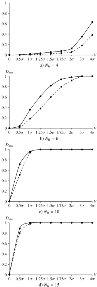
Dtrue=Nexc/N1 exp, (8) whereNexc is the number of exceedings of the critical valueλcr for the substitutional methods of maximum likelihood or fcrfor the method with f-criterion. CPTD estimation is determined for the various number of framesNfr and various values of the ap-parent motion velocity moduleV.
Figure 1 (α = 10−3) shows the curves of near-zero apparent motion detected by different methods: the Fisher
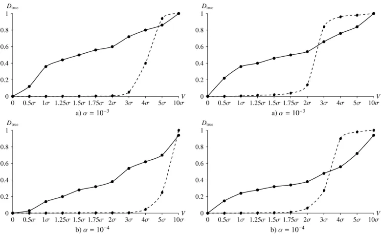
f-criterion (5) method (curve 1); substitutional method for max-imum likelihood detection using the known variance of the po-sition measurements (C.12) (curve 2); and substitutional method for maximum likelihood detection using external estimation of rms error (C.13) ˆσout=0.15 (curve 3) and ˆσout=0.25 (curve 4). Figure2(α=10−3) shows the curves of near-zero apparent motion detection obtained by the Fisher f-criterion method (5) with the critical tabulated value fcr of the Fisher distribution statistics with (w,Nmea−r) degrees of freedom (Phillips 1982) and the critical valuefcraccording to the predefined significance levelα.
A method of in situ modeling for analysis of indicators of quality of the near-zero apparent motion detection on a series
of CCD-frames.In this case, it is impossible to restore the real
law of the errors’ distribution completely. The method of in situ modeling is, therefore, more appropriate (Kuzmyn 2000).
We compiled the set of objects with practically zero apparent motion in the framework of the CoLiTec project (Savanevych et al. 2015a,b) and used it as the internal catalog (IC) of motionless objects in a series of frames (Vavilova et al. 2012a).
V Dtrue
0 0.5σ 1σ 1.25σ1.5σ1.75σ 2σ 3σ 4σ
0 0.2 0.4 0.6 0.8 1
1 2
3 4
a)Nfr=4
V Dtrue
0 0.5σ 1σ 1.25σ1.5σ1.75σ 2σ 3σ 4σ
0 0.2 0.4 0.6 0.8 1
1 2
3
4
b)Nfr=6
V Dtrue
0 0.5σ 1σ 1.25σ1.5σ1.75σ 2σ 3σ 4σ
0 0.2 0.4 0.6 0.8 1
1 2
3
4
c)Nfr=10
V Dtrue
0 0.5σ 1σ 1.25σ1.5σ1.75σ 2σ 3σ 4σ
0 0.2 0.4 0.6 0.8 1
1
2 3
4
d)Nfr=15
Fig. 1.Curves of the near-zero apparent motion detection obtained by the method using Fisherf-criterion (1), substitutional methods with the known variance (2), with external estimations of rms error 0.15 (3) and rms error 0.25 (4).
V Dtrue
0 0.5σ 1σ 1.25σ1.5σ1.75σ 2σ 3σ 4σ
0 0.2 0.4 0.6 0.8 1
a)Nfr=4
V Dtrue
0 0.5σ 1σ 1.25σ1.5σ1.75σ 2σ 3σ 4σ
0 0.2 0.4 0.6 0.8 1
b)Nfr=6
V Dtrue
0 0.5σ 1σ 1.25σ1.5σ1.75σ 2σ 3σ 4σ
0 0.2 0.4 0.6 0.8 1
c)Nfr=10
V Dtrue
0 0.5σ 1σ 1.25σ1.5σ1.75σ 2σ 3σ 4σ
0 0.2 0.4 0.6 0.8 1
d)Nfr=15
V Dtrue
0 0.5σ 1σ 1.25σ1.5σ1.75σ 2σ 3σ 4σ 5σ 10σ
0 0.2 0.4 0.6 0.8 1
a)α=10−3
V Dtrue
0 0.5σ 1σ 1.25σ1.5σ1.75σ 2σ 3σ 4σ 5σ 10σ
0 0.2 0.4 0.6 0.8 1
b)α=10−4
Fig. 3. Curves of the near-zero apparent motion detection with the SANTEL-400AN telescope obtained by the Fisher f-criterion method (solid line) and by the substitutional method with external estimation of rms error 0.15 (dashed line).
evaluations of their errors. These values can be used in the in situ modeling.
Further, these deviations should be added to the determined values of the object’s displacements according to their velocities of the apparent motion. Thereby, it is possible to use the real laws of the positional errors distribution in the study of their motion by the in situ modeling method.
In situ data. Series of CCD-frames from observatories
ISON-NM (MPC code – “H15”; Molotov et al. 2009) and ISON-Kislovodsk (MPC code – “D00”;ISON-Kislovodsk 2016) were selected as the in situ data. The ISON-NM observatory is equipped with a 40 cm telescope SANTEL-400AN with CCD-camera FLI ML09000-65 (3056×3056 pixels, the pixel size is 12 microns). Exposure time was 150 s.
The ISON-Kislovodsk observatory is equipped with a 19.2 cm wide-field telescope GENON (VT-78) with CCD-camera FLI ML09000-65 (4008 × 2672 pixels, the pixel size is 9 microns). Exposure time was 180 s. Figures 3 and 4 show the curves of the near-zero apparent motion detection obtained by the Fisher f-criterion (5) and by the substitutional method of maximum likelihood with an external estimation of rms error (C.13) for two sources of in situ data.
Analysis of indicators of quality of the near-zero apparent motion detection in a series of CCD-frames by the method of
sta-tistical modeling.Analyzing different approaches, we can note
that the substitutional methods of maximum likelihood detection with known variance of the object’s position (C.12) depicted by the curve 2 in Fig.1, and the methods with external estimation of rms errors ˆσout =0.15 (C.13) represented by the curve 3 in the
V Dtrue
0 0.5σ 1σ 1.25σ1.5σ1.75σ 2σ 3σ 4σ 5σ 10σ
0 0.2 0.4 0.6 0.8 1
a)α=10−3
V Dtrue
0 0.5σ 1σ 1.25σ1.5σ1.75σ 2σ 3σ 4σ 5σ 10σ
0 0.2 0.4 0.6 0.8 1
b)α=10−4
Fig. 4. Curves of the near-zero apparent motion detection with the GENON (VT-78) telescope obtained by the Fisher f-criterion method (solid line) and by the substitutional method with external estimation of rms error 0.15 (dashed line).
same figure are the most sensitive to the object velocity changes. For example, CPTD of the near-zero apparent motion for these methods increases in the series consisting of four frames and havingV = 0.5σ. Here,σis an rms error of the errors of esti-mated positions. For other methods the velocity module of the apparent motion is not less thanV =1.25σ, and ifNfr=6, not less thanV=σ.
The curve 1 in Fig. 1 demonstrates that the near-zero ap-parent motion detection method with Fisher f-criterion (5) is not effective enough with the data of statistical modeling, when the number of frames Nfr is small. But if Nfr is not less than eight, this method is not inferior to other ones by CPTD. In own turn, the substitutional method of maximum likelihood with the known variance of the object’s position (C.12) exists only in theory and can not be applied in practice.
Hereby, the substitutional method of maximum likelihood with external estimation of rms error (C.13) described by curve 3 in Fig.1is the most effective and flexible. We remember that the external estimation can be obtained from measurements of the other objects in CCD-frame.
On the other hand, the determination of critical values for all substitutional methods encounters formidable obstacles. First of all, it is not clear how to separate a set of stars (objects with a zero rate motion) from the objects with a near-zero apparent motion to determine them. Also, this process is very time- and resource-consuming and difficult to apply in rapidly changing conditions of observations in modern asteroid surveys.
In statistical modeling, the critical values fcr of the
Table 1.Information about observatories and telescopes at which the CoLiTec software is installed.
Observatory ISON-Uzhgorod Observatory
Cerro Tololo Inter-American Observatory
(CTIO)
ISON-Kislovodsk Observatory
MPC code K99 – – D00
Telescope ChV-400 BRC-250M Promt8 Santel-400AN Aperture, cm 40 25 61 40
CCD-camera FLI PL09000
Apogee
Alta U9 Apogee F42
FLI
ML09000-65 Resolution, pix 3056×3056 3072×2048 2048×2048 3056×3056 Pixel size,µm 12 9 13.5 12 Scale,00 1.42 1.46 0.66 2.06
levels are almost equal to the tabulated critical values of Fisher distribution statistics with (w, Nmea −r) degrees of freedom (Phillips 1982;Melard 2014) of the method (5). It is obviously seen in Fig.2. Moreover, these figures demonstrate that the simi-larity of these critical values of decisive statistic does not depend on the number of frames in the series.
Hence, it is not necessary to determine them for the different number of framesNfrand observation conditions. It is enough to use the maximum allowable tabulated value (Melard 2014).
Following from our statistical experiments, we can note that the method for the near-zero apparent motion detection with Fisher f-criterion (5) is more effective for the large number of CCD-frames and the velocity module of the apparent motion
V =0.5σas it’s seen in Fig.2.
Analysis of indicators of quality of the near-zero apparent motion detection in a series of CCD-frames by the method of
in situ modeling.It is found that the method for detection of the
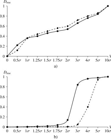
object’s near-zero apparent motion using Fisherf-criterion (5) is the most sensitive to changes in the object’s velocity (Figs.3,4). As shown earlier, CPTD for this method increases when series includes four frames or more and whenV = 0.5σ. For other methods the velocity module of the apparent motion should be not less thanV=1.25σ.
In addition, the method of the near-zero apparent motion de-tection using Fisher f-criterion (5) is stable and does not depend on the kind of telescope (Fig.5a). Therefore, there is no need to undertake additional steps for determining the critical value of the decisive statistic after the equipment replacement or obser-vational conditions change. Other methods of the apparent mo-tion detecmo-tion encounter problems when determining the critical values as it is obvious from Fig.5b.
Examples of objects discovered by the method of near-zero apparent motion detection in a series of CCD-frames using
sig-nificance criteria of the apparent motion. There are many of
objects with near-zero apparent motion that were detected by the CoLiTec software for automated asteroids and comets dis-coveries (Savanevych et al. 2015b). The plugin implements the method of detection using the Fisher f-criterion (5). Table 1 gives information about several observatories at which the Co-LiTec software is installed. The real-life examples of detec-tion of asteroids 1917, 6063, 242211, 3288 and 1980, 20460, 138846, 166 with a near-zero apparent motion are described in Tables2and3, respectively.
The observations were conducted in 2017 in the period from 3 to 19 July with different small telescopes and confirmed an efficiency of the method even in bad conditions (strong backlight from the full Moon).
V Dtrue
0 0.5σ 1σ 1.25σ1.5σ1.75σ 2σ 3σ 4σ 5σ 10σ
0 0.2 0.4 0.6 0.8 1
a)
V Dtrue
0 0.5σ 1σ 1.25σ1.5σ1.75σ 2σ 3σ 4σ 5σ 10σ
0 0.2 0.4 0.6 0.8 1
b)
Fig. 5. Curves of the near-zero apparent motion detection with the GENON (VT-78) (solid line) and SANTEL-400AN (dashed line) tele-scopes (α = 10−3) obtained by the Fisher f-criterion method (a), substitutional method for maximum likelihood detection with external estimation of rms error (b).
Tables 2 and3 contain the following apparent motion pa-rameters of the aforementioned asteroids: date of observations; name of telescope; exposure time during the observation; ap-parent velocities of object along each coordinate ˆVx and ˆVy in the rectangular coordinate system (CS; see, Appendix C, formu-las (C.1), (C.2)); apparent velocities of objects ˆVRAand ˆVDEin the equatorial CS determined from the observational data; ap-parent velocities of object ˆVRAcat and ˆVDEcat in the equatorial CS determined from the Horizons system (Giorgini et al. 2001) for the same times of observation; velocity module ˆV of the ap-parent motion of object determined from the observational data ( ˆV=
q
ˆ
V2
x+Vˆy2); velocity module ˆVcatof the apparent motion of object determined from the Horizons system; average FWHM of object in five frames; average S/N of object in five frames; rms error of stars positional estimates ˆσ0(C.7) from UCAC4 catalog (Zacharias et al. 2013) with S/N approximately equal to the ob-ject’s S/N; brightnessMagcatof the object determined from the Horizons system; angular distance between the observed aster-oid and the Moon; phase of the Moon, percentage illumination by the Sun; coefficient of the velocity module ˆVcatof the appar-ent motion of object determined in relative terms, in other words, rms error of measurement deviations of the object’s position (k=Vˆ/σˆ0).
Discovery of the sungrazing comet C/2012 S1 (ISON).On
Table 2.Examples of asteroids 1917, 6063, 242211, 3288 with a near-zero apparent motion that were detected by the proposed method using Fisherf-criterion (5).
Parametersobjects 1917 6063 242211 3288
Date of observation 2017-07-11
2017-07-11
2017-07-13
2017-07-19 Telescope Promt8 Promt8 Promt8 Promt8 Exposure, s 80 40 40 20
ˆ
Vx, pix/fr 0.47 0.94 –0.56 0.01
ˆ
Vy, pix/fr –0.47 0.73 0.36 –0.47 ˆ
VRA,00/fr –0.49 0.66 –0.30 –0.22
ˆ
VDE,00/fr –0.25 0.65 –0.39 –0.02
ˆ
VRAcat,00/fr –0.32 0.66 –0.22 –0.31
ˆ
VDEcat,00/fr –0.34 0.65 –0.37 –0.04
ˆ
V, pix/fr 0.66 1.19 0.67 0.50
ˆ
V,00/fr 0.55 0.93 0.49 0.22
Vcat,00/fr 0.47 0.93 0.43 0.31
Average FWHM, pix 3.48 3.68 4.62 5.70 Average S/N,00/fr 6.86 10.04 12.83 11.86
ˆ
σ0, pix (UCAC4) 0.40 0.45 0.41 0.30
ˆ
σ0,00 0.30 0.19 0.28 0.20
Magcat,m 18.2 17.38 17.17 18.24
Asteroid-Moon dist.,
deg 97 82.5 68 91.5
Moon phase % 91 91 76 14
k=Vˆ/σˆ0 1.65 2.64 1.63 1.67
Table 3.Examples of asteroids 1980, 20460, 138846, 166 with a near-zero apparent motion that were detected by the proposed method using Fisherf-criterion (5).
Parametersobjects 1980 20460 138846 166
Date of observation 2017-07-09
2017-07-03
2017-07-13
2017-07-19
Telescope
BRC-250M ChV-400 ChV-400 ChV-400 Exposure, s 30 30 60 60
ˆ
Vx, pix/fr 0.06 0.72 –0.06 –0.11
ˆ
Vy, pix/fr 0.37 0.51 0.58 –0.21 ˆ
VRA,00/fr –0.11 –1.09 0.07 0.19
ˆ
VDE,00/fr –0.61 0.76 1.34 –0.32
ˆ
VRAcat,00/fr 0.09 –1.06 0.13 0.14
ˆ
VDEcat,00/fr –0.52 0.88 0.83 –0.28
ˆ
V, pix/fr 0.37 0.88 0.59 0.24
ˆ
V,00/fr 0.62 1.33 1.35 0.31
Vcat,00/fr 0.53 1.38 0.84 0.38
Average FWHM, pix 3.35 4.59 5.12 4.92 Average S/N,00/fr 10.31 7.76 7.26 42.14
ˆ
σ0, pix (UCAC4) 0.38 0.39 0.39 0.26
ˆ
σ0,00 0.54 0.62 0.57 0.36
Magcat,m 15.32 15.91 16.56 13.71
Asteroid-Moon dist.,
deg 67.5 79.5 83.5 84
Moon phase % 99 79 76 14
k=Vˆ/σˆ0 0.97 2.26 1.51 0.92
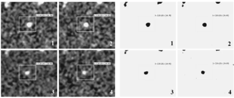
Network (ISON) project (Molotov et al. 2009; Minor Planet Center 2012). Information about observatory and telescope is available in Table1. At the moment of discovery, the magnitude of the comet was equal to 18.8m, and its coma had 10 arc sec-onds in diameter that correspsec-onds to 50 000 km at a heliocentric distance of 6.75 au. Its apparent motion velocity at the moment of discovery was equal to 0.8 pixels per frame. The size of the comet image in the frame was about five pixels. In Fig.7a the cell size corresponds to the size of the pixel and is equal to 2 arc sec-onds. Within 26 min of the observation, the image of the comet has been moved by three pixels in the series of 4 CCD-frames (Fig.7b).
C/2012 S1 (ISON) comet (Fig. 8) was detected using the CoLiTec software for automated asteroids and comets discov-eries (Savanevych et al. 2015b) with the implemented method of detection using Fisher f-criterion (5). C/2012 S1 (ISON) comet was disintegrated at an extremely small perihelion distance
a) b)
Fig. 6.Sungrazing comet C/2012 S1 (ISON) at the moment of discovery in the center of crop of CCD-frame with field of view 20×20 arcmin (panel a), 8×8 arcminutes (panel b).
a) b)
Fig. 7.Panel a: images of C/2012 S1 (ISON) comet on CCD-frames: the image size is five pixels (a), the shift of comet image between the first and the fourth CCD-frames of series is three pixels (panel b).
Fig. 8.Sungrazing comet C/2012 S1 (ISON) in a series of four CCD-frames.
of about 1 million km on the day of perihelion passage, on November 28, 2013. Its disintegration was caused by the Sun’s tidal forces and the significant mass loss due to the alterations in the moments of inertia of its nucleus. Despite having a short visible life time for our observations, this comet supplemented our knowledge of cometary astronomy.
5. Conclusions
We proposed a computational method for the detection of objects with the near-zero apparent motion on a series of CCD-frames, which is based on the Fisher f-criterion (Phillips 1982) instead of using the traditional decision rules that based on the maximum likelihood criterion (Myung 2003).
The statistical modeling showed that the most effective and adaptive method for the apparent motion detection is the substi-tutional method of maximum likelihood using the external es-timation of rms errors (C.13, Fig.1). But the process of deter-mining the critical values of decisive statistics is very time- and resource-consuming in the rapidly changing observational con-ditions. By this reason, we recommended to apply the method of the near-zero apparent motion detection for the subclass of ob-jects with 3σ-velocity using Fisher f-criterion (5) for series with the number of frames Nfr = 4 or more (Fig.1). The condition of a large number of frames in the series also makes the pro-posed method not inferior to other methods of apparent motion detection by CPTD.
When studying the indicators of quality of near-zero appar-ent motion detection by the in situ modeling method the objects from the internal catalog fixed on a series of CCD-frames were used as in situ data. It was found that in the case when the ve-locity does not exceed 3 rms errors in object position per frame, the most effective method for near-zero apparent motion detec-tion is the method which uses Fisher f-criterion (Figs. 3, 4). When compared with other methods, this method is stable at the equipment replacement (Fig.5).
The proposed method for detection of the objects with 3σ-velocity apparent motion using Fisher f-criterion was ver-ified by authors and implemented in the embedded plugin de-veloped in the CoLiTec software for automated discovery of asteroids and comets (Savanevych et al. 2015b).
Among the other objects detected and discovered with this plugin, there was the sungrazing comet C/2012 S1 (ISON; Minor Planet Center2012). The velocity of the comet apparent motion at the moment of discovery was equal to 0.8 pixels per CCD-frame. Image size of the comet on the frame was about five pix-els (Fig. 7a). Within 26 min of the observation, the image of the comet had moved by three pixels in the series of four CCD-frames (Fig.7b). So, it was considered to belong to the subclass of SSOs that have a velocity of apparent motion between CCD-frames not exceeding three rms errors σ of measurements of its position (ε = 3σ). In total, about 15% of SSO objects with ε-velocity apparent motion in the CCD-frames. These are the objects beyond the Jupiter’s orbit as well as asteroids heading straight to the Earth.
Acknowledgements. The authors thank observatories that have implemented CoLiTec software for observations. We especially thank Vitaly Nevski and Artyom Novichonok for their discovery of ISON comet and others SSOs. We are grateful to the reviewer for their helpful remarks that improved our paper and, in particular, for the suggestion “to add a few real-life examples, where the method provides a detection of motion for an object that would otherwise be difficult to detect”. We express our gratitude to Mr. W. Thuillot, coordinator of theGaia-FUN-SSO network (Thuillot et al. 2014), for the approval of CoLiTec as a well-adapted software to the Gaia-FUN-SSO conditions of observation (https://gaiafunsso.imcce.fr). Research is supported by the APVV-15-0458 grant and the VVGS-2016-72608 internal grant of the Faculty of Science, P. J. Safarik University in Kosice (Slovakia). The CoLiTec software is available
onhttp://neoastrosoft.com.
References
Arora, J. S., & Haug, M. W. 1994,Structural Optimization, 8, 69
Barnard, K., Connolly, A., Denneau, L., et al. 2006,Proc. SPIE, 6270, 627024 Burden, R. L., & Faires J. D. 2010, Numerical Analysis, Brook Cole, 9th edn.
(Academic Press), 888
Catalina Sky Survey 2016,http://www.lpl.arizona.edu/css Dailey, J., Bauer, J., Grav, T., et al. 2010,BAAS, 41, 817
Dubovsky, P. A., Briukhovetskyi, O. B., Khlamov, S. V., et al. 2017, OEJV, 180 Elenin, L., Savanevych, V., & Bryukhovetskiy, A. 2013,Minor Planet Circ.,
82692, 1
Elenin, L., et al. 2014, Asteroids, Comets, Meteors (University of Helsinki) Garcia, J., Besada, J. A., Molina, J. M., et al. 2008, TI-WDC/ESAV. IEEE, 1 Genovese, A. F. 2001,Johns Hopkins APL Technical Digest, 22, 614 Giorgini, J. D., Chodas, P. W., & Yeomans, D. K. 2001,BAAS, 33, 1562 Gong C., & McNally D. 2004, in AIAA Guidance, Navigation, and Control
Conference and Exhibit, 432
Gunawan, S., & Panos Y. 2006,J. Mech. Des., 129, 158 Heasley, J. N., Jedicke, R., & Magnier, E. 2007,BAAS, 39, 806 Hsieh, H., Kaluna, H. M., Novakovi´c, B., et al. 2013,AJ, 771, 1 ISON-Kislovodsk 2016, Astronomy and telescope making,
http://astronomer.ru
Ivashchenko, Yu., Kyrylenko, D., & Gerashchenko, O. 2013,Minor Planet Circ., 82554, 3
Jedicke, R., Denneau, L., Granvik, M., & Wainscoat, R. 2009, Proc. of the Advanced Maui Optical and Space Surveillance Technologies Conf., 43 Johnson, N. L., Kotz, S., & Balakrishnan, N. 1995, Continuous Univariate
Distributions, 2nd edn. (Wiley)
Kuzmyn, S. Z. 2000, Tsyfrovaia radyolokatsyia, Vvedenye v teoryiu (Kyiv), 428 Lee, M. D., & Wagenmakers, E.-J. 2014, Bayesian Cognitive Modeling: A
Practical Course (Cambridge University Press), 284
Lehman, E. L., & Romano, J. P. 2010, Testing Statistical Hypotheses, 3rd edn. (Springer), 768
Marsaglia, G., & Tsang, W. W. 2000,J. Stat. Software, 8, 1 Masson, M. E. J. 2011,Behavior Research Methods, 43, 679 Melard, G. 2014,Comput. Stat., 29, 1095
Miller, P. J., Jeffrey, D. W., Holmes, R. E., et al. 2008,Astron. Ed. Rev. 7, 57 Minor Planet Center 2012, COMET C/2012 S1 ISON
http://www.minorplanetcenter.org/mpec/K12/K12S63.html Miura N., Kazuyuki I., & Naoshi B. 2005,AJ, 130, 1278
Molotov, I., Agapov, V., Kouprianov, V., et al. 2009,Proc. of the 5th European Conf. on Space Debris, ESA SP-672, 7
Morey, R. D., & Wagenmakers, E.-J. 2014,Stat. Prob. Lett., 92, 121
Myers, A. J., Pierfederici, F., Axelrod, T., et al. 2008,AAS/DPS meeting, 40, 52.06
Myung, I. J. 2003,J. Math. Psych., 47, 90 Park, S. Y., & Bera, A. K. 2011, J. Econ., 219
Parker, A., & Kavelaars, J. 2009, AAS/DPS meeting, 41, 47.10 Phillips, P. C. B. 1982,Biometrika, 69, 261
Pohorelov, A. V., Khlamov, S. V., Savanevych, V. E., et al. 2016,Odessa Astron. Publ., 29, 136
Raab, H. 2012, Astrophysics Source Code Library [record ascl:1203.012] Sanders-Reed J. N. 2005,AJ, 130, 1278
Savanevych, V. E. 1999,Radio Electronics and Informatics, 1, 4
Savanevych, V. E. 2006, Models and the data processing techniques for detection and estimation of parameters of the trajectories of a compact group of space small objects, Manuscript for Dr. Sc. (KhNURE, Kharkiv), 446
Savanevych, V. E., Briukhovetskyi, O. B., Sokovikova, N. S., et al. 2012,Space Sci. Technol., 18, 39
Savanevych, V. E., Briukhovetskyi, O. B., Sokovikova, N. S., et al. 2015a, MNRAS, 451, 3287
Savanevych, V. E., Briukhovetskyi, O. B., Sokovikova, N. S., et al. 2015b, Kinematics and Physics of Celestial Bodies, 31, 302
Shucker, B. D., & Stuart, J. S. 2008,Asteroids, Comets, Meteors, 1405, 8388 Stokes, G. H., von Braun, C., Sridharan, R., et al. 1998,Lincoln Lab. J., 11, 27 Stokes, G. H., Evans, J. B., Viggh, H. E. M., et al. 2000,Icarus, 148, 21 Thuillot, W., Carry, B., Berthier, J., et al. 2014, Proc. of the Annual meeting of
the French Society of Astronomy and Astrophysics, SF2A-2014, 445 Troianskyi, V. V., Bazyey, A. A., Kashuba, V. I., et al. 2014,Odessa Astron.
Publ., 27, 154
Vavilova, I. B. 2016,Odessa Astron. Publ., 29, 109
Vavilova, I. B., Pakulyak, L. K., Shlyapnikov, A. A., et al. 2012a,Kinematics and Physics of Celestial Bodies, 28, 85
Vavilova, I. B., Pakuliak, L. K., Protsyuk, Yu. I., et al. 2012b,Balt. Astron., 21, 356
Appendix A: Model of the motion parameters
The model of rectilinear and uniform motion of an object along each coordinate independently can be represented with the set of equations:
xk(θx) = x0+Vx(τk−τ0); (A.1) yk(θy) = y0+Vy(τk−τ0), (A.2) wherek(i,n)=kis the index number of measurement in the set, namely,ith measurement ofnfrth CCD-frame with the observed object;x0,y0are the coordinates of object from the set of mea-surements at the timeτ0of the base frame timing;Vx,Vyare the apparent velocities of object along each coordinate:
θx = (x0,Vx)T; (A.3)
θy = (y0,Vy)T; (A.4)
are the vectors of the parameters of the apparent motion of the object along each coordinate, respectively.
The measured coordinatesxk,ykat the timeτkare also de-termined by the parameters of the apparent motion of object in CCD-frame and can be calculated according to Eqs. (A.1) and (A.2).
So, the set ofNfrmeasurements ofnfrth frame timing at the timeτn is generated from observations of a certain area of the celestial sphere. One frame of the series is a base CCD-frame, and time of its anchoring is the base frame timingτ0. The aster-oid image onnfrth frame has no differences from the images of stars on the same frame. Results of intra-frame processing (one object per CCD-frame) can be presented as theYinmeasurement (ith measurement on the nfrth frame). In general, the ith mea-surement on the nfrth frame contains estimates of coordinates
YKin={xin;yin}and brightnessAinof the object:Yin={YKin;Ain}. We used a rectangular coordinate system (CS) with the center lo-cated in the upper left corner of CCD-frame. It is assumed that all the positional measurements of the object are previously trans-formed into coordinate system of the base CCD-frame.
A set of measurements (no more than one in the frame), be-longing to the object, has the form as follows:
Ωset = (YK1(i,1), ...,YKk(i,n), ...,YKNmea(i,N f r))
= ((x1, y1), ...,(xk, yk), ...,(xNmea, yNmea)), (A.5) whereNmea is the number of the position measurements of the object in Nfr frames. MeasurementsYk from the setΩset (A.5) of measurements are selected by the rule of no more than one measurement per frame. Measurements of the object positions can not be obtained in all CCD-frames. Therefore, the number of measurements which belong to the object in certain set of measurements will generally be equal toNmea(Nmea≤Nfr).
It is supposed that the observational conditions are practi-cally unchanged during observations of object with near-zero ap-parent motion. So, the rms errors of estimates of its coordinates in the different CCD-frames are almost identical. Deviations of estimates of coordinates of this object, which belong to the same setΩsetof measurements, are independent of each other both in-side the one measurement and between measurements obtained in different frames. Deviations of coordinates are normally dis-tributed (Kuzmyn 2000), have a zero mathematical expectation and unknown variances (standard deviations)σ2
x,σ2y.
Appendix B: Likelihood function for detection of a near-zero apparent motion
This common density distribution forH0hypothesis (1), assum-ing that the object is a star with zero rate apparent motion, is
defined as follows:
f0( ¯x,y, σ¯ )= Nmea
Y
k=1
[Nxk( ¯x, σ2)Nyk( ¯y, σ2)], (B.1)
where ¯x, ¯y are the coordinates of the object; Nz(mz, σ2) = 1
√
2πσexp(− 1
2σ2(z−mz)2) is the density of normal distribution with mathematical expectationmzand varianceσ2inzpoint.
The common density distribution for H1 hypothesis (2) is defined otherwise. Namely, the coordinates xk(θx),yk(θy) at the timeτk, calculated from Eqs. (A.1) and (A.2), must be used in-stead of the object’s position parameters ¯x, ¯y:
f1(θ, σ)=
Nmea
Y
k=1
[Nxk(xk(θx), σ2)Nyk(yk(θy), σ2)]. (B.2)
Absence of information on the position of the object, its appar-ent motion and variance of estimates of object position in a set of measurements leads to the necessity of using the substitu-tional decision rule (Lehman et al. 2010;Morey et al. 2014). In this case, the statistics for distinguishing these hypotheses is the LR estimate ˆλ(Ωset) (Morey et al. 2014).
Appendix C: Evaluation of parameters for substitutional methods of maximum likelihood detection of a near-zero apparent motion
OLS-evaluation of the parameters of the object’s apparent mo-tion may be represented in the scalar form (Kuzmyn 2000):
ˆ
x0 =
DAx−CBx
NmeaD−C2
; ˆVx=
NmeaBx−CAx
NmeaD−C2
; (C.1)
ˆ y0 =
DAy−CBy
NmeaD−C2
; ˆVy=
NmeaBy−CAy
NmeaD−C2
, (C.2)
whereAx= Nmea
P
k=1
xk;Ay=
Nmea
P
k=1
yk;Bx= Nmea
P
k=1∆
τkxk;By= Nmea
P
k=1∆
τkyk;
C =
Nmea
P
k=1∆
τk; D = Nmea
P
k=1∆ 2
τk; ∆τk = (τk−τ0) is the difference between the timeτ0of the base frame and timeτkof the frame, in which thekth measurement is obtained.
The interpolated coordinates of the object in thekth frame are represented as
ˆ
xk = xˆk(ˆθx)=xˆ0(ˆθx)+Vˆx(ˆθx)(τk−τ0); (C.3) ˆ
yk = ykˆ (ˆθy)=yˆ0(ˆθy)+Vˆy(ˆθy)(τk−τ0). (C.4)
Thus, for each (kth) measurement from Nmea measurements of the setΩset(A.5), we have:
– the unknown real position of the objectxk(θx),yk(θy);
– the measured object coordinates xk,ykat the timeτkin the coordinate system of the base frame;
– the interpolated coordinates ( ˆxk,yˆk)= xˆk(ˆθx), ˆyk(ˆθy) defined by Eqs. (C.3) and (C.4).
The variance of the object’s positional estimates in a set of
mea-surements.Using the measuredxk,yk(A.1), (A.2) and the
ˆ σ2
xand ˆσ2y(hereinafter – variances) of the object’s positions can be represented as:
ˆ σ2
x =
Nmea
X
k=1
(xk−xˆk(ˆθx))2/(Nmea−m); (C.5)
ˆ σ2
y =
Nmea
X
k=1
(yk−yˆk(ˆθy))2/(Nmea−m), (C.6)
wherem=2 is the number of parameters of the apparent motion along each coordinate in a set of measurements.
Assuming the validity of the hypothesis about zero (H0) and near-zero (H1) apparent motions, the conditional variances ˆσ2
0, ˆ
σ2
1of the object’s position can be represented as: ˆ
σ2 0 =
R20
2(Nmea−m)
; (C.7)
ˆ σ2
1=
R21
2(Nmea−m)
, (C.8)
where
R20 =
Nmea
X
k=1
((xk−xˆ¯)2+(yk−yˆ¯)2); (C.9)
R21 =
Nmea
X
k=1
((xk−xˆk(ˆθx))2+(yk−yˆk(ˆθy))2), (C.10)
are the residual sums of the squared deviations of object’s positions (Burden et al. 2010).
We note also that the variance of the positions in a set of measurements can be obtained by the external data, for exam-ple, from measurements of another objects on a series of CCD-frames. Hence, the required estimate is a variance estimation of all position measurements of objects detected in CCD-frame and identified in any astrometric catalog.
Substitutional methods for maximum likelihood detection of
a near-zero apparent motionmay operate with unknown real
po-sitionxk(θx),yk(θy) of the object at a timeτkand unknown
vari-ancesσ2
x,σ2yof the object’s position in CCD-frames.
It is easy to show that in the latter case the substitutional method can be represented as
R2
0−R 2 1
R20R21 ≥
ln(λcr)
ANmea
, (C.11)
whereλcr is the maximum allowable (critical) value of the LR estimate for the detection of a near-zero apparent motion;A =
2(Nmea−m).
If the varianceσ2of the object’s position is known, the sub-stitutional method can be represented as
R20−R21≥2σ2ln(λcr). (C.12)
In that case, if the external variance estimation ˆσ2
out of the posi-tion is used, the substituposi-tional method takes the form:
R2
0−R 2 1 ˆ σ2
out