The Blum medial linking structure for multi-region analysis

(1)

The Blum Medial Linking Structure for Multi–Region Analysis

Ellen Gasparovic

A dissertation submitted to the faculty of the University of North Carolina at Chapel Hill in partial fulfillment of the requirements for the degree of Doctor of Philosophy in the Department of Mathematics.

Chapel Hill 2012

Approved by

(2)

Abstract

ELLEN GASPAROVIC: The Blum Medial Linking Structure for Multi–Region Analysis (Under the direction of James Damon)

The Blum medial axis of a region with smooth boundary in _Rn+1 _{is a skeleton-like}

(3)

Acknowledgements

First and foremost, I owe my deepest gratitude to my advisor, Jim Damon, for his enthusiasm and guidance throughout the years. I truly appreciate his great patience and thorough feedback. Many thanks to my committee members — Pat Eberlein, Jane Hawkins, Steve Pizer, and Richard Rimanyi — for their insights and numerous helpful conversations.

I am very grateful for the generous support of Carol and Ed Smithwick, who funded my dissertation completion fellowship through the Royster Society of Fellows.

I must thank the members of the UNC and the College of the Holy Cross mathematics departments, especially my undergraduate advisor, Tom Cecil, who encouraged me to pursue a doctorate in mathematics.

Thank you, too, to my office mates and friends in graduate school for all of the laughter and fun times we have had together.

(4)

List of Tables

Table 3.1. Generic linking for medial axes in _R2_{. . . 54}

Table 3.2. Generic linking for medial axes in _R3_{. . . 54}

Table 5.1. Generic linking type of codimension 4 in _R4_{. . . 112}

Table 5.2. Generic linking type of codimension 5 in _R5. . . 113

Table 5.3. Generic linking type of codimension 6 in _R6. . . 114

(8)

List of Figures

1.1. Generic medial axis strata in _R3_. _{. . . 22}

2.1. Example of an abstract neighborhood. . . 29

2.2. Computing integrals over regions Γ⊂Ω as medial integrals. . . 33

2.3. 2D discrete m–rep used for segmentation of the brainstem [42]. . . 36

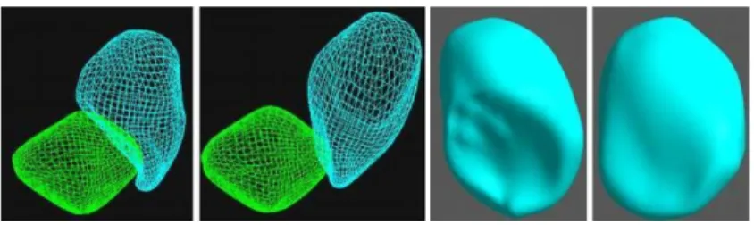
2.4. Discrete m–rep of the kidney and 3D rendering (courtesy of Medical Image Display and Analysis Group at UNC). . . 36

2.5. Example of discrete m–reps of a complex of organs. . . 37

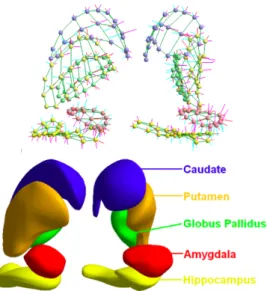
2.6. A second example of a multi–object complex. . . 38

3.1. Non–linked portions of regions. . . 46

3.2. Example demonstrating the dual roles of boundary points in _R3_. _{. . . 47}

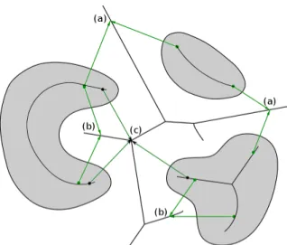
3.3. Illustration of (a) linking between distinct regions, (b) self-linking, and (c) partial linking. . . 48

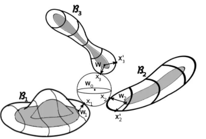
3.4. Linking between three regions in _R3. . . 48

3.5. Example illustrating generic linking possibilities, including self-linking, in R2. . . 55

3.6. Stratification refinement example. . . 57

3.7. More on the refinement example. . . 57

3.8. Example of generic linking between three distinct regions in _R3_. _{. . . 60}

3.9. A portion of the refined stratification for Figure 3.8. . . 60

3.10. A collection of linking vector fields in _R2. . . 62

6.1. Example of a region Γ over which one may integrate. . . 126

6.2. Illustration for measuring closeness. . . 130

6.3. Illustration of relative significance of regions. . . 131

(9)

Introduction

We consider a collection of objects in _Rn+1 _{modeled by disjoint regions with smooth}

boundaries. For example, such a collection of regions in_R2 or_R3 can be used to model a collection of objects in a 2D or 3D medical image, which may consist of organs, glands, arteries, bones, etc. The analysis of one object in the image can be improved using knowledge of its geometrical relation to neighboring objects (see, e.g., [24] [30] [41]). Our objective is to introduce a structure which will capture both the geometric and shape properties of the individual objects as well as their “positional geometry,” which captures the geometry of the regions relative to one another.

In the case of a single region Ω ⊂ _Rn+1 _{with smooth boundary} _{B, there have been}

a number of approaches to capturing the shape of Ω. These include the chordal locus of Brady and Asada [5], the arc–segment medial axis of Leyton [28], the symmetry set of Bruce, Giblin, and Gibson [8], and the Blum medial axis [2] [3]. Each of these is a skeletal–like structure in Ω which captures shape properties. However, the Blum medial axis has proven to be the most useful, and it is the structure we will be extending to a configuration of regions. The concept of the medial axis was introduced by Blum, an engineer, in 1967 [2] [3], and was later independently introduced by Milman as thecentral set [38]. TheBlum medial axis M of Ω is the locus of centers of spheres in Ω which are tangent to B at two or more points (or have a degenerate tangency). On M is defined a multivalued vector field U from points of M to the points of tangency.

(10)

“medial geometry” of the radial vector field on M completely captures the local and global geometry of the boundary and the region [13] [14] [15]. Third, a discrete version of the Blum medial axis and radial vector field, known as a discrete “m–rep” (see [42] and the many references in [43]), has been an especially effective tool for problems in medical imaging.

Our goal in introducing the Blum medial linking structure is to extend these advan-tages to configurations of multiple regions. The linking structure provides a means of relating the individual medial axes to one another and to the medial axis of the comple-mentary region. First, we use singularity theory to classify the local normal forms of the medial linking structure for generic configurations of regions in dimensions n ≤ 6. The genericity results in the multi–region setting require proving a transversality theorem for families of “multi–distance functions” defined on a collection of hypersurfaces, which extends that of Looijenga [29] for a single distance function used in Mather’s proof. This will require that multiple transversality statements for different distance functions be satisfied at the same points. It is this simultaneity that brings in additional subtleties not present in the case of a single distance function.

Second, we extend the medial geometry of a single region to the entire configuration of regions including their complement. This leads into the third goal of applying the linking structure to address questions from mathematics and medical imaging for multi– region shape analysis; these questions are enumerated in Section 2.6 of Chapter 2. We identify invariants of the positional geometry of a configuration of regions, which may be computed directly from the linking structure, and construct a “tiered graph” structure involving the invariants that measures order of importance among regions.

(11)

(12)

CHAPTER 1

Determining the Generic Structure of the Blum Medial Axis

Using Singularity Theory

1.1. Introduction

The objective of this chapter is to present the details of the classification of the generic structure of the Blum medial axis of a single region. The first half of the chapter focuses on many of the fundamental definitions and theorems from singularity theory as developed by Thom [44] and Mather [32] (see also [10], [31], [36]). In Section 1.2, we recall the notion of right–equivalence of function germs, as well as the notion of a versal unfolding of such a germ and the infinitesimal criterion for versality. Then, in Section 1.3, we examine the relationship between versality and transversality.

In the second half of the chapter, we introduce the Blum medial axis as the Maxwell set of the family of distance squared functions associated to a given hypersurface in_Rn+1_.

In Section 1.4, we present a transversality theorem due to Looijenga [29], which Mather [32] applied to completely classify for dimensions n ≤ 6 the generic structure of the Maxwell set. (Yomdin [47] gave a classification for n ≤ 3 using a different method.) We define Whitney stratified sets in Section 1.5 and give a specific description of the stratification we obtain in_R3. In Section 1.6, we finish with some remarks on the various notions of codimension that we shall use in this thesis.

1.2. R+₋_{equivalence and versal unfoldings}

(13)

Let X be a smooth n–dimensional manifold and let x ∈ X. Consider the smooth functions f : U1 → R and g : U2 → R where U1 and U2 are open neighborhoods of

x in X. We say that f, g are locally equivalent at x if there exists a neighborhood x ∈ U ⊂ U1 ∩U2 such that f|U = g|U. This defines an equivalence relation. A local

equivalence class at x is called a germ of a smooth function at (X, x). We denote the germ determined by the function f by f : (X, x)→(_R, y) with f(x) =y.

We can extend this notation to a finite setS ={x1, . . . , xr}ofr distinct points inX. Two smooth functions f :U1 →Rand g :U2 →RwithU1, U2 open and S ⊂U1∩U2 are

locally equivalent at S if there is an open U,S ⊂U ⊂U1∩U2, so that f|U =g|U. This

again forms an equivalence relation, and an equivalence class, denotedf : (X, S)→(_R, y) with f(xi) = y for i= 1, . . . , r, is called a multigerm of a smooth function at S.

By choosing local coordinates at x ∈ X, we may now reduce to the case X = _Rn_. The set of germs atxof smooth functions (_Rn_{, x)}_→

Rform a local ring which we denote

by Ex, with maximal ideal mx consisting of germs (_Rn, x) → (_R,0). In the special case that x = 0, we let En denote the ring of germs at the origin and mn its unique maximal ideal. Ifx= (x(1)_{, . . . , x}(n)_{) denote coordinates on}

Rn, Hadamard’s Lemma implies that

x(1), . . . , x(n) (viewed as function germs) generate the maximal ideal mn [7]. Similarly, let ES denote the ring of multigerms of smooth functions at S ={x1, . . . , xr}, so that if Exi denotes the ring of germs of smooth functions at xi ∈R

n _for _i_{= 1, . . . , r,}

ES =Ex1 ⊕. . .⊕ Exr.

Also, letmS =mx1⊕. . .⊕mxr. Thus, the multigermf : (R

n_{, S)}_→₍

R, y) may be viewed

as the r-tuple (f1, . . . , fr), where for each i, fi : (Rn, xi)→(R, y) is a germ of a smooth function at xi ∈Rn.

(14)

Definition 1.2.1. (a) Letf, g ∈ Ex. We say f isright–equivalent, or R–equivalent, to g if there exists a germ of a diffeomorphism φ : (_Rn_{, x)}_→₍

Rn, x) satisfying

f =g◦φ.

We say f isR+_{–equivalent} _to _g _{if, for some constant} _c_∈

R and φ as above,

f =g◦φ+c.

(b) Two smooth multigerms f, g ∈ ES are said to be R–equivalent if there exists a multigerm of a smooth diffeomorphism φ : (_Rn_{, S)} _→ ₍

Rn, S), with φ(xi) = xi for 1 ≤ i≤r, such that

f =g◦φ.

With such a φ, f and g are said to be R+_{–equivalent} _if

f =g◦φ+c

for some c∈ _R. That is, letting f = (f1, . . . , fr), g = (g1, . . . , gr), and φ = (φ1, . . . , φr), the statement that f is R+_{-equivalent to} _g _{translates to}

(f1, . . . , fr) = (g1◦φ1+c, . . . , gr◦φr+c).

Observe that R–equivalence for multigerms requires that the value of f and g at the points ofS be the same, whileR+_{−equivalence allows}_f _and_g _{to each take on a different}

value at S.

Next, we introduce the notion of an unfolding family of functions of an initial multi-germ f.

Definition 1.2.2. For f ∈ ES, the smooth map germ

F : (_Rn×_Rs_,_(S,₀₎₎_→

R,

(15)

with F0(x) = f(x) is said to be an s–parameter unfolding of f.

Following [10], let R+

un(s) denote the group of s–parameter unfoldings, which acts on s–parameter unfoldings of germs f ∈ ES.

Definition 1.2.3. LetF, G: (_Rn_×

Rs,(S,0)) →Rbe unfoldings of f ∈ ES. The families F, G are said to be R+

un−equivalent if there exists a multigerm of a diffeomorphism

Φ : (_Rn×_Rs_,_(S,₀₎₎ _→₍

Rn×Rs,(S,0)),

(x, w)7→(φ1(x, w),Ψ(w)),

and a smooth function germ C : (_Rs_,₀₎_→

R such that

F(x, w) =G(φ1(x, w),Ψ(w)) +C(w).

Definition 1.2.4. Suppose F is an s–parameter unfolding of f ∈ ES, while G is a p–parameter unfolding of f. A mapping from G to F consists of a smooth germ ψ : (_Rp_,₀₎_→₍

Rs,0) such that the unfolding

ψ∗F : (_Rn×_Rp,(S,0))→_R,

(x, w)7→F(x, ψ(w))

is R+

un−equivalent to G. The unfolding ψ∗F is called the pullback of F by ψ.

We arrive at the definition of aversal unfolding.

Definition 1.2.5. LetF : (_Rn×_Rs_,_(S,₀₎₎_→

Rbe an unfolding of the smooth multigerm

f ∈ ES. ThenF is said to be versalif, for any other unfoldingG: (Rn×Rp,(S,0))→R of f, there exists ψ : (_Rp_,₀₎_→₍

Rs,0) such that G and ψ∗F are R+un–equivalent.

(16)

Define in En the Jacobian ideal

(1.1) J(f) = h∂fi=En·

∂f ∂x1

, . . . , ∂f ∂xn

and the_R–vector subspace

(1.2) h∂Fi=_R·

∂F ∂u1 _u₌₀

, . . . , ∂F ∂us

_u₌₀

.

The extended tangent space to the R+_{−orbit of} _f _is

(1.3) TR+

ef =h∂fi+h1i

and theextended normal space to the R+_{−orbit of} _f _{is the space}

(1.4) NR+

e ·f =En/TR+e ·f.

(The usual tangent space is given by TR+_f ₌ _m

n ·

∂f ∂x1

, . . . , ∂f ∂xn

+h1i, but the extended tangent space removes the restriction that 0 must map to 0.)

Definition 1.2.6. Let f ∈ En. The R+e–codimension of f is

R+

e–codim(f) =dimR NR +

e ·f.

Definition 1.2.7. Let F be an unfolding of the germ f at x ∈ _Rn_{. We say} _F _{is an} infinitesimally R+_{−versal unfolding} _of _f _if

En=TR+e ·f +h∂Fi.

Next, we give the analogous definitions in the multigerm setting. Let F be an s– parameter unfolding of f = (f1, . . . , fr) ∈ ES, so that F = (F1, . . . , Fr) where Fi is an unfolding of fi for every i= 1, . . . , r. Define in ES the ideal

(17)

and the vector subspace

h∂Fi=h∂1F, . . . , ∂sFi,

where ∂jF = (∂jF1, . . . , ∂jFr) forj = 1, . . . , sand ∂jFi = ∂Fi ∂uj

u=0

for every i= 1, . . . , r. As in the single germ setting, the extended tangent space to the R+_{−orbit of} _f _is

(1.5) TR+

ef =h∂fi+h1i,

the extended normal space to the R+_{−orbit of} _f _{is the space}

(1.6) NR+

e ·f =ES/TR+e ·f,

and theextended R+_{−codimension of} _f _{is defined as in Definition 1.2.6.}

Definition 1.2.8. Let F be an unfolding of f ∈ ES. Then F is an infinitesimally R+_{−versal unfolding} _of _f _if

ES =TR+e ·f+h∂Fi.

For both single and multigerms, we have the following fundamental theorem which was stated for germs by Thom [44] and proven by Mather ([33]). The version for multigerms was stated by Mather in [32] and a proof follows from the general unfolding theorem in [16].

Theorem 1.2.9. An unfolding is versal if and only if it is infinitesimally versal.

Thus, the infinitesimal criterion for versality implies that the R+

e−codimension of f gives the minimum number of parameters that are needed for f to be versally unfolded. A versal unfolding F is said to be miniversal if F has the least possible number of parameters.

(18)

Corollary 1.2.10. Letf ∈ En. Suppose theRe+−codimension off iss, and letw1, . . . , ws be a basis for NR+

e ·f. Then

F(x, u) =f(x) +u1w1(x) +. . .+usws(x)

is a miniversal unfolding of f.

Mather proved the following essential theorem on the uniqueness of versal unfoldings, which follows from Theorem 1.2.9.

Theorem 1.2.11 (Mather [33]). Any two s–parameter R+_{−miniversal unfoldings are}

isomorphic.

Therefore, any miniversal unfolding has an algebraic normal form. Moreover, any p– parameter versal unfolding G with p > s is isomorphic to the unfolding F ×idp−s with F as in Corollary 1.2.10, soG will also have a polynomial normal form.

In addition to the uniqueness theorem, there is another important theorem regarding versality which establishes its openness property.

Theorem 1.2.12. Let F : (_Rn × _Rs_,_(S,₀₎₎ _→

R be an R+−versal unfolding of the

multigerm f ∈ ES, and let

Σ(F) =

(x, w)∈_Rn_×

Rs: ∂F

∂x(i)(x, w) = 0, i= 1, . . . , n

be the critical set of the unfolding. Then there exist neighborhoods W of 0in _Rs andU of S in _Rn _{so that, for all} _w_∈_W _and _S0 _⊂_Σ(F₎_∩_(U _{× {w}),} _F _{: (}

Rn×Rs,(S0, w))→R

is an R+_{−versal unfolding.}

Finally, we introduce the notion of finite determinacy of germs [36], which requires the notion of a k–jet of a smooth function. If f : (_Rn_{, x)} _→

R is a smooth germ, the

k–jet off atx, denoted jkf(x), is the list of derivatives

(19)

which is equivalent to giving the k–th order Taylor expansion of f at x.

Definition 1.2.13. Let f ∈ En and suppose that, for some positive integer k, any g ∈ En with jkf(0) = jkg(0) is R+−equivalent to f. Then f is said to be finitely k– determined for R+_{−equivalence.}

Finite determinacy of f implies that it is sufficient to study the k–jet of a finitely de-termined germ to determine its singularity theoretic properties. If f, g ∈ En (or ES) are R+_{−equivalent germs, then}_f _is_{k–determined if and only if} _g _{is [}₃₆_{]. We conclude with}

a final theorem involving finite determinacy.

Theorem 1.2.14 (Mather [36]). A germ f ∈ En (or ES) is finitely determined if and only if f is of finite R+_{−codimension.}

Consequently, by the infinitesimal criterion for versality, a germ f has an _R+–versal unfolding if and only iff is finitely determined.

In Section 1.3, we shall examine more consequences and fundamental theorems of versality.

1.3. Versality and transversality

There is a fundamental relationship between versality of unfoldings and transversality to certain submanifolds of jet space. Before delving into this relationship, we briefly recall some notation related to jet spaces (see, e.g., [23]).

For smooth manifolds Xn _and _Yp_{, let} _Jk_{(X, Y}_{) denote the} _{k–jet bundle of maps} X → Y with base X and fiber Jk(_Rn,_R)x, the space of jets of functions _Rn → _R at the point x∈_Rn_{. Alternatively,} _Jk_{(X, Y}_{) may be viewed as a bundle over} _X _×_Y _with fiber consisting of k–jets of mappings (_Rn,0)→(_Rp,0), which we denote by Jk(n, p). If f :X →Y is smooth,

(20)

denotes the k–jet extension mapping, which is also smooth. Let α : Jk_{(X, Y}₎ _→ _X and β : Jk_{(X, Y}₎ _→ _Y _{denote the source and target mappings, respectively. Next, let} X(r) =X×. . .×X

| {z }

rtimes

\∆X, where ∆X is the generalized diagonal in Xr, i.e.,

∆X ={(x1, . . . , xr)∈Xr : xi =xj for some i6=j}.

The r–multi k–jet bundle is rJk(X, Y) with fiber rJk(X, Y)S for S = {x1, . . . , xr} and base X(r)_{, and the} _r–multi _{k–jet extension of} _f _:_X _→_Y _is

rjkf :X(r)→rJk(X, Y)

(x1, . . . , xr)7→rjkf(x1, . . . , xr) = (jkf(x1), . . . , jkf(xr).

The groupR(k) _of _{k-jets of diffeomorphism germs}

Rn →Rn acts algebraically on the

jet space fiber Jk(_Rn,_R)x. Namely, if jkφ ∈ R(k), z ∈ Jk(Rn,R) with f ∈ En such that jk_f _{is a representative of} _{z, and} _c_∈

R, then the action is given by

(1.7) jkφ·z =jk(f ◦φ) +c.

We obtain a natural action on the multijet space fiber rJk(Rn,R)S in the analogous way, i.e., if φ = (φ1, . . . , φr) is a multigerm of a diffeomorphism atS, z = (z1, . . . , zr)∈ rJk(Rn,R)S with jkfi a representative of zi for i= 1, . . . , r, and c∈R, we have

(1.8) jkφ·z = (jk(f1◦φ1) +c, . . . , jk(fr◦φr) +c).

(21)

Definition 1.3.1. (a) The smooth germ f : (_Rn_,₀₎ _→ ₍

R,0) is said to have an Ak singularity at 0 for some positive integer k if f isR+_{−equivalent to the smooth germ}

g = n−1 X

i=1

±x2

i ±x k+1

n .

(b) The smooth multigerm f : (_Rn, S)→(_R,0) with S ={x1, . . . , xr} is said to have an

Aβ singularity at S for an r−tuple β ={k1, . . . , kr} if f is R+−equivalent to

g = n−1 X

i=1

(x₁(i))2+ (x₁(n))k1+1_{, . . . ,}

n−1 X

i=1

(x(_ri))2+ (x(_rn))kr+1 !

,

where (x(1)_i , . . . , x_i(n)) are coordinates on the i-th copy of _Rn _for _i_{= 1, . . . , r.}

These are the only simple multigerms with each germ having a local minimum at 0. In part (b) above, source coordinates may be chosen independently around each xi ∈S so thatxi is locally the origin in each copy ofRn. As we shall see in the next section, theAk and Aβ singularities are the relevant orbits for the classification of the generic structure of the medial axis.

Remark 1.3.2. Other examples of submanifolds of jet space include theThom-Boardman singularity submanifolds. For a smooth map f : X → Y with Xn and Yp smooth manifolds, we may decompose the source spaceX by singularity type off in the following way. Let corank(f) = min(n, p)−(rank(f) at x), and define

Si(f) ={x∈X :corank(f) =i}.

If f has corank 0, the k-jet of f is said to be regular. Thom proved that the sets Si_(f) are submanifolds of X [27]. Similarly, we may define the sets

(22)

for some nonnegative integer j; continuing the process inductively, we define, for the sequence I ={i1, ..., ij}with integers i1 ≥. . .≥ij ≥0, the sets

SI(f) =Sj(f|Si1,...,ij−1_(f)).

In [4], Boardman proved that a set of the form SI_{(f) is a manifold by finding a} subman-ifold ΣI_{(X, Y}_{) of} _Jk_{(X, Y}_{) such that the jet extension mapping}

jkf :X →Jk(X, Y)

satisfies jk_f

t ΣI_{(X, Y}_{) and} _jk_f−1_(ΣI_{(X, Y}_{)) =} _SI_(f_{). We refer to the submanifold} ΣI_{(X, Y}_{) as the}_{Boardman manifold with symbol} _{I. Let Σ}I _{denote the fiber of Σ}I_{(X, Y}_), and let Σ1j = Σ1,...,1 with 1 appearing j times.

Now, let F be an s–parameter unfolding of f ∈ En. The k–jet extension of F is the mapping

j₁kF :_Rn×_Rs_→_Jk₍

Rn,R),

(x, u)7→j₁kF(x, u) =jkF(·, u)(x),

so that the subscript “1” indicates the jet is taken with respect to the coordinates on_Rn_. There is a natural algebraic identification of this jet space as

(1.9) Jk(_Rn,_R)x ∼=En/mkn+1

(see, e.g., [37]), and the fiber Jk_(n,_{1) is identified with}

(23)

Likewise, suppose F denotes an s–parameter unfolding of the multigerm f ∈ ES. The r–multi k–jet extension of F is the mapping

rj1kF : (Rn)(r)×Rs→rJk(Rn,R), (x1, . . . , xr, u)7→rj1kF(x, u) = (j

k_F_{(·, u)(x}

1), . . . , jkF(·, u)(xr)).

We come now to the important theorem that enables one to express the condition that F be a versal unfolding of f ∈ ES as a transversality statement.

Theorem 1.3.3 ([32]). Let F be an s-parameter unfolding of f ∈ ES. Then F is an R+_{−versal unfolding of} _f _{if and only if}

rj1kF is transverse to the orbit of rj1kF(S,0) in

rJk(Rn,R) under the action of rR+ for sufficiently large k.

1.4. The generic structure of Blum medial axis for n≤6

In this section, we present a variant of Thom’s transversality theorem due to Looi-jenga, as well as an extension of it due to Wall, which apply to families of distance squared functions. Looijenga’s theorem yields a complete classification of the generic structure of the Blum medial axis in dimensions n ≤6. The genericity results hold for a residual set of embeddings, and are proven by demonstrating transversality of a jet extension of a mapping to certain submanifolds of a jet space, then applying the transversality theorem.

1.4.1. Looijenga’s transversality theorem and distance–genericity. Suppose X is a smooth, compact, connected, n-dimensional manifold, and φ :X ,→_Rn+1 _{a smooth}

embedding. Let

σφ:X×Rn+1 →R, (1.11)

(24)

be the family of squared distance functions, and let

rj1kσφ:X(r)×Rn+1×V →rJk(X,R)

(x1, . . . , xr, w, v)7→(j1k(||Φ(·, v)−w|| 2_(x

1), . . . , j1k(||Φ(·, v)−w|| 2_(x

r))

denote the r–multi k–jet extension of σφ. Looijenga’s transversality theorem applies to a certain class of submanifolds W of the multijet space rJk(X,R): those W which are invariant under addition of constants. This means that, for anyc∈_R,z = (z1, . . . , zr)∈ W implies that (z1+c, . . . , zr+c)∈W.

Theorem 1.4.1 (Looijenga [29], [45]). Let W be a smooth submanifold of rJk(X,R) that is invariant under addition of constants. Then

H={φ∈Emb(X,_Rn+1) :rj1kσφ is transverse to W}

is a residual set in the C∞ topology. If X is compact, the set is open and dense.

We refer to the elements of H as distance-generic embeddings. In [45], Wall proved an extension of Looijenga’s theorem. Let Sn⊂_Rn+1 _{denote the unit} _{n–sphere, let}_X _and _φ

be as in the statement of Theorem 1.4.1, and define the family of height functions

hφ :X×Sn →R, (1.12)

(x, w)7→w·φ(x).

Theorem 1.4.2. Let W be a smooth submanifold of rJk(X,R) that is invariant under addition of constants. Then

H={φ∈Emb(X,_Rn+1) :rj1khφ is transverse to W}

is a residual set in the C∞ topology. If X is compact, the set is open and dense.

(25)

Then, we explain how Looijenga’s transversality theorem allows its generic structure to be determined.

Definition 1.4.3. Given a smooth manifold N and a smooth family F : N ×_Rs _→

R,

the Maxwell set of F is the set of parameters w ∈ _Rs _{such that} _F_{(·, w)} _{attains an} absolute minimum value at more than one distinct point in N or at a degenerate critical point.

Let φ : X ,→ _Rn+1 _{be a smooth embedding of a smooth compact, connected,}

n-dimensional manifold X, where φ(X) =B is the boundary of a smooth, compact, con-nected region Ω⊂ _Rn+1 _{by the Jordan–Brouwer Separation Theorem. Then the medial}

axis of Ω is the part of the Maxwell set of σφ (defined in (1.11)) that lies in Ω.

Mather and Yomdin classified the generic local normal forms of the medial axis, Yomdin for dimension n ≤3 [47] and Mather for n ≤6 [32]. Moduli appear in dimen-sion 7 and higher, preventing further smooth classification (although a classification by topological equivalence becomes possible). Of the simple singularities, only the A2k+1

singularities as defined in Definition 1.3.1 are relevant to the classification as they are the only simple singularities that have local minima.

Theorem 1.4.4 (Mather [32], Yomdin [47]). For n ≤ 6, let X be a smooth, compact, connected, n-dimensional manifold, and let φ : X ,→ _Rn+1 _{be a smooth embedding with}

φ(X) = B, where B=∂Ω. Locally, the Maxwell set ofσφis diffeomorphic to the Maxwell set of the R+_{−versal unfolding of one of the following germs:}

• (1≤n ≤6) A2

1, A31, A3,

• (2≤n ≤6) A4₁, A1A3,

• (3≤n ≤6) A5

1, A5, A21A3,

• (4≤n ≤6) A6₁, A1A5, A23, A31A3,

• (n = 5,6) A7

1, A21A5, A1A23, A41A3, A7,

• (n = 6) A8

(26)

Remark 1.4.5. Mather actually classified the generic normal forms for the family of distance functions, rather than distance squared. However, the normal forms are the same if one replaces the family of distance functions with the family of distance squared functions, which is smooth, due to the fact that these families are R+_{−equivalent as}

unfoldings and therefore have the same types of critical points.

1.5. Stratifications of the medial axis M and boundary B

In this section, we explain how to obtain stratifications of the boundary B and Blum medial axis M of a region Ω ⊂ _Rn+1 _{arising from the singular behavior related to the}

Maxwell set of the family of distance squared functions. We first recall the notion of a Whitney stratification, then give the specific details of the boundary and medial axis stratifications in _R3_.

1.5.1. Whitney stratifications. In this section, we recall the notation of a stratified space and, in particular, a Whitney stratified space.

Definition 1.5.1. A closed set M ⊂ _Rn+1 _{is a} _{stratified set} _if _M _{may be written}

as the union of a locally finite collection of smooth, locally closed, disjoint submanifolds

Sα ⊂ Rn+1, α ∈ I, where I is a partially ordered index set. The submanifolds, called strata, must satisfy the axiom of the frontier: Sα∩Sβ 6=∅ if and only if Sα ⊂ Sβ and α≤β, where Sβ denotes the closure of Sβ in Rn+1.

Definition 1.5.2. A closed setM ⊂_Rn+1 _{is a} _{Whitney stratified set}_{with a Whitney}

stratification S = {Sα}α∈I if M is a stratified set with all pairs of strata satisfying the Whitney regularity conditions (a) and (b), defined as follows. Given a pair of

strata Sα and Sβ with Sα ⊂Sβ, suppose {xi} is a sequence of points in Sβ converging to y ∈Sα, and {yi} a sequence of points in Sα also converging to y. Denote by τ the limit of the sequence of tangent spaces TxiSβ, and let r denote the limiting secant line of the

(27)

Mather proved that Whitney’s condition (b) implies condition (a) [34]. The sequences in Definition 1.5.2 may not have limits; however, by choosing subsequences, we may assume they converge.

In Chapter 5, we shall obtain refinements in the following sense of the stratifications of a collection of boundaries of regions and their medial axes.

Definition 1.5.3. A refinement T = {Tγ}γ∈J of a stratification S = {Sα}α∈I is a stratification such that every stratum Sα is a union of some collection of strata from T.

1.5.2. Stratification of the critical set of family of distance squared functions.

In this section, under the hypotheses of Theorem 1.4.4, we describe the stratification C of the singular set of the family of distance squared functions σφ.

For values of n ≤ 6, there is a canonical rR+-invariant stratification of the multijet space rJk(X,R) consisting of strata which are orbits under the action of rR+ on r– multi k-jets of germs with simple singularities (see [33], [37]). Orbits under an algebraic group action form a Whitney stratification where they are locally finite, so the canonical stratification of jet space is Whitney. For a distance–generic embeddingφ, Theorem 1.4.1 implies that the multijet extension mapping

rj1kσφ:X(r)×Rn+1 →rJk(X,R)

is transverse to this stratification for sufficiently high k. This implies that the pull-back of the stratification toX(r)_×

Rn+1 underrj1kσφ is also Whitney stratified with strata of the form rj1kσ

−1

φ (Wi), where Wi is a stratum in rJk(X,R) [34]. Since the stratification of rJk(X,R) satisfies the boundary condition, so does the pull-back of the stratification;

that is, if Wj belongs to the closure of the stratum Wi in rJk(X,R), then rj1kσ

−1

φ (Wj) belongs to the closure of rj1kσ

−1

φ (Wi).

(28)

one to determine the explicit relationship between the stratification on the medial axis M and the stratification on B to which it corresponds. Let Si ={x1, . . . , xr} with each xi ∈Rn, and suppose

(1.13) F : (_Rn×_Rp_,_(S,₀₎₎_→₍

R,0), Fw(x) =F(x, w)

is a versal unfolding of the multigerm F0 =f of singularity typeAβ. By the openness of versality (Theorem 1.2.12), since F is versal in a neighborhood of (S,0), nearby germs of f are also versally unfolded. Consider the real algebraic set

(1.14) {(x1, . . . , xk, w) :Fw has a critical point at xj, F(xj, w) = y∀j}

for different values ofk. It is a real algebraic set sinceF is versal and it is defined by the following algebraic conditions on polynomials:

∂Fw ∂x (x)

x=xj

= 0, F(xj, w)−y= 0 for j = 1, . . . , k.

Therefore, it is Whitney stratified with the stratification inherited from the pull-back of the canonical stratification of jet space.

For each set of the form in (1.14), its projections onto both _Rn and _Rp yield semi-algebraic sets by the Tarski-Seidenberg Theorem [27]; therefore, they are also Whitney stratified by singularity type of Fw. Moreover, the combined images of these projections will provide the local models for the stratifications of B and M, respectively, since the singular sets of σφ and F0 :=F ×idn+1−p are locally diffeomorphic.

The versality theorem ensures that the projection of the stratum of the singular set of σφcorresponding toAβ singularity type to the parameter spaceRn+1will be smooth. Let

χAβ ⊂ M denote this projection. In addition, we can project the stratum to X, which

is diffeomorphic to B under the diffeomorphism φ provides. So, let ΣAβ ⊂ B denote the

(29)

stratum on M under a radial flow that is smooth on the strata of the medial axis; see Section 2.3 in Chapter 2.

1.5.3. Explicit stratifications of M and B in _R3_. _{In this section, we determine the}

local structure of the stratifications of M and B in _R3 _{using the generic local normal}

forms ofσφ given in Theorem 1.4.4.

First, we determine the local models of the χ_Ak

1 strata on M and the ΣAk1 strata on

B for k = 2,3,4. LetF = (F1, . . . , Fk) be the standard R+−miniversal unfolding of the Ak₁ multigerm, i.e.,

F1 = (x (1) 1 )

2_{+ (x}(2) 1 )

2₊_u 1,

.. .

Fk−1 = (x(1)_k−1) 2

+ (x(2)_k₋₁)2+uk−1,

Fk = (x

(1)

k )

2_{+ (x}(2)

k )

2_.

Forj = 1, . . . , k, Fj has a critical point at x

(1)

j =x

(2)

j = 0 with critical value uj forj < k and critical value 0 forFk. Thek functions have equal minima whenu1 =. . .=uk−1 = 0,

and graphing this gives the Ak₁ stratum. To obtain the entire local model, we equate 2≤j < k of the critical values and set them less than or equal to the remaining critical values. By Theorem 1.2.11, σφis isomorphic to F0 :=F ×id3−k. The codimension in R3 of the χ_Ak

1 stratum is k−1, the extendedR

+_{−codimension of the multigerm.}

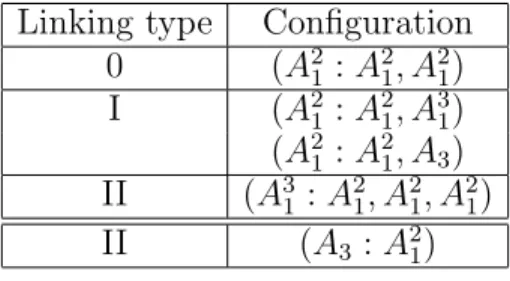
For k = 2, the local models of the χ_A2

1 and ΣA21 strata are smooth sheets. When

k = 3, the local model of the χ_A3

1 stratum on M consists of three half-planes meeting

along a curve, called a Y-branch curve. See Figure 1.1. The corresponding Σ_A3

1 stratum

onBconsists of three smooth curves associated to the same branch curve onM. Finally, the local model of the χ_A4

1 stratum on M is a single point, called a 6-junction point,

occurring at the intersection of four branch curves and six half-planes. See Figure 1.1. Using the radial flow, we conclude that the Σ_A4

(30)

which has three mutually transverse curves passing through it that correspond to three distinct branch curves on M.

Next, we determine the local models of the χA3 stratum on M and the ΣA3 stratum

onB. Let

F =x4₁+u1x12+u2x1+x22

be the standard 2–parameter R+_{−miniversal unfolding of an} _A

3 singularity. This

func-tion has a critical point provided that 4x3

1 + 2u1x1 +u2 = 0 and x2 = 0. A direct

computation shows that, in order to obtain minima, we must have u2 = 0 and u1 ≤ 0

(specifically, it turns out that u1 = −2x21 to have a minimum). The versal unfolding σ

is isomorphic to F0 = F ×id1. Since u3 is a free parameter in R3, the local model is

a half-plane that is bounded by a curve, known as an edge curve on the medial axis. See Figure 1.1. An edge curve on the medial axis corresponds to the ΣA3 stratum on

the boundary, which is a crest curve consisting of points such that the larger principal curvature in absolute value at each point is a maximum along the associated principal direction (see, e.g., [9]).

The local models of the χA1A3 stratum on M and the corresponding ΣA1A3 stratum

on B are similarly established. See Figure 1.1 for the local model of the χA1A3 stratum

on M, called a fin point, which is a point at which a branch curve and an edge curve intersect and end.

(31)

1.6. A note on the notions of codimension

In this dissertation, we shall refer to several types of codimension: theR+

e−codimension of a (germ or) multigerm of singularity type Aβ as defined in Definition 1.2.6; the codi-mension as a submanifold of jet space of the orbit of the multigerm under therR+–action; the codimension in _Rn+1 _{of the medial axis stratum} _χ

Aβ; and the codimension in B of

the corresponding boundary stratum ΣAβ. In this section, we explain the relationships

that exist among these various notions of codimension.

Suppose the family of distance squared functions σφ : (X ×Rn+1,(S, w0)) → (R, z)

is a versal unfolding of the multigerm σφ(·, w0) : (X, S) → (R, z) of singularity type

Aβ with |S| = r. First, recall that the R+

e−codimension of a multigerm of singularity typeAβ, which we denote byR+e–codim(Aβ), equals the number of unfolding parameters in its miniversal unfolding. If codim_Rn+1(χ_A

β) denotes the codimension in R

n+1 _{of the}

corresponding medial axis stratumχAβ, we know from Section 1.5 that

codim_Rn+1(χ_A

β) =R +

e–codim(Aβ). (1.15)

Second, as mentioned in Section 1.5.2, there is a radial flow on the medial axis that provides a diffeomorphism betweenχAβ and the corresponding stratum on the boundary

ΣAβ. Therefore, since ΣAβ and χAβ have the same dimension, and since the codimension

in B of the ΣAβ stratum, denoted codimB(ΣAβ), equals n−dim(ΣAβ), it follows from

(1.15) that

codimB(ΣAβ) = codimRn+1(χAβ)−1

(1.16)

=R+

e–codim(Aβ)−1.

Third, by the equivalence of versality and transversality, the mappingrj1kσ at (S, w0)

is necessarily transverse to the orbit of rj₁kσ(S, w0) under the rR+ group action on jet

space. We let Wβ _{denote this orbit, and let codim}

JS(Wβ) denote the codimension of

(32)

codimension and the jet space codimension (see, e.g., [8]):

(1.17) codimJS(Wβ) =R+e–codim(Aβ) +nr.

We first explain briefly why this relation holds in the r = 1 case. For f ∈ En, we know that R+

e–codim(f) = dimREn/J(f)−1, and

mnJ(f)/mkn+1

represents the orbit of the k–jet of f in the jet space fiber mn/mkn+1 [10]. Then the codimension of this orbit in mn/mk+1

n is given by

dim_R mn/mkn+1

mnJ(f)/mkn+1

= dim_R(mn/mnJ(f))

= dim_R(mn/J(f)) +n = dim_R(En/J(f))−1 +n =R+

e–codim(f) +n. (1.18)

The fact that dim_R(mn/mnJ(f)) = dim_R(mn/J(f)) is due to the fact that f has an isolated singularity and therefore the ideal J(f)/mnJ(f) is of finite codimension, i.e., dim_R(J(f)/mnJ(f)) =n.

For a multigermf = (f1, . . . , fr) with anAβ singularity, we consider the codimension of its orbit Wβ _{as a submanifold in} _E

n/mkn+1

r

, the multijet space fiber. Using (1.18) and the fact that the values of each of the fi’s are necessarily equal, we have that the codimension of Wβ _in _E

n/mkn+1

r

is

(r−1) + r

X

i=1

(R+_e–codim(fi) +n).

Then, since R+

e–codim(f) = r

X

i=1

R+

(33)

CHAPTER 2

Medial Geometry for a Single Region

2.1. Introduction

In this chapter, we present a survey of the results for the medial geometry of a single region as they apply to the Blum medial axis, with the goal in Chapter 6 of extending these results to configurations of multiple regions. The Blum medial axis is viewed as a Whitney stratified set M on which is defined a (multivalued) radial vector field U, defined from points on M to the points of tangency on the boundary. This is a special case of a skeletal structure. Earlier work focused on relating the differential geometry of the boundary of a region with the differential geometry of the medial axis involving derivatives of the radius function. Damon [14] [15] offered a more direct approach to studying the geometric properties of a region and its boundary via the medial geometry of the radial vector field on the medial axis. This involves two variations on the ordinary differential geometric shape operator and is related to the geometry of the region and its boundary via a radial flow, as we shall see in Sections 2.2 — 2.4.

(34)

2.2. The radial vector field

In this section, we recall the definition and properties of the radial vector field U defined on the Blum medial axisM of a compact, connected, orientable region Ω⊂_Rn+1

with smooth boundary B.

Let Mreg denote the set of regular points of M that belong to the top–dimensional

strata of M, and let Msing denote the union of all remaining strata. These singular

points consist of (1) the set of non–edge points, (2) the set of edge points belonging to the boundary ofM, denoted∂M, and (3) the set of edge closure points belonging to the closure of the boundary of M, denoted ∂M).

The radial vector field U on M is a multivalued vector field with one value at each pointx0 ∈M for each of the associated tangency points on the boundaryB. LetU =r·u,

where u is a multivalued unit vector field on M and the radial function r is a positive multivalued function on M, or a function which takes one value at each point for each of the values of U. A smooth value of the vector field U at a smooth point x0 ∈ M is

a neighborhood V of x0 together with a choice of values of the vector field on V that

constitute a smooth vector field on V.

The radial vector field satisfies the following properties (see [40] and [14]):

(1) (Behavior at smooth points) For any smooth pointx0 ∈M, there are two values

ofU that have the same length and make the same angle with the tangent space Tx0M. The values of U corresponding to one side of a neighborhood V of x0

form a smooth vector field.

(2) (Behavior at edge points) For any point x0 ∈ ∂M, there is a single value of U

that points away from M and is tangent to the smooth stratum containing x0

in the closure.

(3) (Behavior at singular, non-edge points) LetB(x0) denote a closed ball of radius

centered at x0 ∈Msing with x0 ∈/ ∂M, and let Mα be alocal component of x0,

(35)

corresponds to each value of U at x0 a connected component Ci of B(x0)\M,

called a local complementary component of M at x0, into which U(x0) locally

points in the sense defined in [14].

We end this section by recalling two shape operators on the medial axis that capture the medial geometry of the radial vector field.

Definition 2.2.1. For a non-edge point x0 ∈ M, v ∈ Tx0M, and a choice of smooth

value of the radial vector field U =ru, define the radial shape operator Srad to be

(2.1) Srad(v) =−projU

∂u

∂v

,

where proj_U denotes projection along U onto the tangent space to the medial axis, Tx0M.

For an edge point x0 ∈ M, v ∈ Tx0M, and a smooth value of U chosen on one side of

M, define the edge shape operator SE to be

(2.2) SE(v) = −proj 0

∂u

∂v

,

where proj 0 denotes projection along U onto Tx0∂M ⊕ hni, for n a unit normal vector

field to M.

Let Sv be the matrix representation of Srad with respect to the basis v = {v1, . . . , vn} (resp., SEv is the matrix representation of SE with respect to the basis {v1, . . . , vn} in

the source, where v1, . . . , vn−1 is a basis for Tx0∂M and vn is a positive multiple of u,

and the basis {v1, . . . , vn−1,n} in the target). Unlike the case of differential geometry,

Srad is not self–adjoint; however, it can be diagonalized and the eigenvalues κr i of Srad

are the principal radial curvatures. Likewise, there are n−1 principal edge curvatures, which are the generalized eigenvalues κE i of (SEv, In−1,1).

2.3. The local and global radial flows

(36)

multivalued and only defined on M, it is not possible to define a global radial flow from M in the usual way. We first introduce the local version of the flow before explaining how to obtain a global version.

Definition 2.3.1. The local radial flow ψ in a neighborhood V of a point x0 ∈M for

a smooth choice of the radial vector field U is given by

ψ :V ×[0,1]→_Rn+1_,

(2.3)

(x, t)7→ψt(x) = ψ(x, t) =x+tU(x).

We refer to ψ1, which maps from a region on M to the corresponding region on the

boundary B, as the radial map.

In order to consider both sides of the medial axis simultaneously, we introduce the notion of the double of the medial axisM, on which a global version of the radial flow is defined.

Definition 2.3.2. The double of the Blum medial axis M, denoted Mf, is the set

f

M ={(x, U0)∈M ×_Rn+1 |U0 is a value of U atx}.

As explained in [14],Mfmay be given a topology in the following way. First, forx₀ ∈M_reg

with a valueU(x0) of the radial vector field and a neighborhoodV of x0, a neighborhood

of (x0, U(x0)) ∈ Mf is given by (V × {U0})∩Mf, where {U0} denotes the values of a

continuous extensionU0 ofU(x0) toV. Next, for a neighborhoodV of a pointx0 ∈Msing

and a choice of radial vectorU(x0) that points into some complementary componentCi, a neighborhood of (x0, U(x0))∈Mfis the intersection of a set (V0∩∂Ci)× {U0}withMf.

Here, V0 ⊂V is a neighborhood ofx0 inRn+1 and {U0}consists of values of a continuous

extension of U(x0) to V0∩∂Ci. Damon referred to the neighborhoods in Mfas abstract

neighborhoods; see Figure 2.1 for an example.

There is a canonical line bundle N on Mfwhich is spanned at a point (x₀, U₀)∈ Mf

(37)

Figure 2.1. Example of an abstract neighborhood.

For (a), the local structure of a 3D medial axis near a fin point. For (b) and (c), the abstract neighborhoods of the two points in Mfcorresponding to the fin point.

{tU0 ∈N : 0≤t≤}. Then the global radial flow is the map

e

ψ :N →_Rn+1, (2.4)

(x0, tU0)7→x0+tU0.

First, it is proven in [14] that there is an > 0 so that the radial flow N → Rn+1 is a diffeomorphism onto a “tubular neighborhood” of M. In order to establish the global nonsingularity of the radial flow, we recall three conditions from [14] that the Blum medial axis satisfies. First, if dr denotes the gradient of the radius function, the compatibility condition at a point x0 ∈M states that the compatibility 1-form

(2.5) ηU(v) =v ·U+dr(v)

vanishes at x0 for any v ∈ Tx0M. The compatibility condition ensures that the radial

vector field is orthogonal to the boundary of the region [14]. Second, at any point x0 ∈ M with x0 ∈/ ∂M, the radial shape operator Srad satisfies the following radial

curvature condition:

(2.6) r <min

1 κri

for all positive principal radial curvaturesκri of Srad.

Third, at anyx0 ∈∂M, the edge shape operatorSE satisfies the followingedge condition:

(2.7) r <min

1 κE i

(38)

In [14], Damon showed that, given the three conditions listed above, the global radial flow is a homeomorphismN1 →Ω (fibering Ω\M with the level sets of the flow) which is

a local diffeomorphism from points (x0, U) withx0 ∈Mreg and a local piecewise smooth

homeomorphism on a neighborhood of a point (x0, U) with x0 ∈Msing [14].

In Chapter 6, we will introduce an extension of the radial flow called thelinking flow. The integrability of the radial flow will apply to the integrability of the linking flow.

2.4. Medial geometry via the radial and edge shape operators

In this section, we recall how the radial and edge shape operators evolve under the radial flow. This enables one to find a matrix representation for the radial shape operator for Bt, the level hypersurface of the radial flow at time t, in terms of the shape operator onM. In Chapter 6, we extend this notion to determine the behavior of the radial shape operator under the linking flow.

Damon proved the following two propositions in [15] (Propositions 2.1 and 2.3, re-spectively).

Proposition 2.4.1. Letx0 ∈Mreg with a smooth value of U and a basis v={v1, . . . , vn} of Tx0M. Suppose

1

tr is not an eigenvalue of the radial shape operator Sv at x0. Then, if ψt(x0) =x00 and v

0 _{denotes the image of} _v _under _dψ

t(x0), the radial shape operator Sv0_t

for Bt at x00 is given by

(2.8) Sv0_t= (I−tr·S_v)−1S_v.

Proposition 2.4.2. Let x0 ∈∂M with a smooth value of U (corresponding to one side of

M), and let v={v1, . . . , vn−1, vn}, where vn =u, be a basis of Tx0M. Suppose

1

tr is not a generalized eigenvalue of (SEv, In−1,1). Then, if ψt(x0) =x00 and v0 ={v1, . . . , vn−1,n}

denotes the image of v under dψt(x0), the radial shape operator Sv0_t forB_t at x0

0 is given

by

(39)

Remark 2.4.3. When t = 1 in the above propositions, one obtains a matrix represen-tation for the regular differential geometric shape operator on the boundary B in terms of the radial and edge shape operators on M. This makes it possible to explicitly relate the principal radial and edge curvatures with the ordinary principal curvatures on the boundary (see Theorem 3.2 and Corollary 3.9 in [15]).

2.5. Blum medial axis as a measure space

Global invariants of a region Ω or its boundaryBare expressed by integrals over these spaces. We explain how such invariants can be computed from the medial geometry as integrals overMfas defined in Definition 2.3.2. In Chapter 6, we shall extend these results

to integrals over the complements of multiple regions.

2.5.1. Introduction to integration over the medial axis. We first explain how to integrate a multivalued function g over the medial axis M, as introduced by Damon in [13]. Such a multivalued functiong lifts to a well-defined functiong_e=g◦π onMf, where

πdenotes the natural projectionπ :Mf→M. Amultivalued measurable (resp.,integrable

orcontinuous)functiongonM is a multivalued function such that_eg is measurable (resp., integrable or continuous) on Mf.

Damon used the Riesz Representation Theorem to prove the existence of a unique regular positive Borel measuredM onMf(Proposition 2.2 in [13]). Then, for a

multival-ued continuous function g on M, the medial integral of _eg on Mf is given by integration

with respect to dM. In the Blum case, this measure

(2.10) dM =ρ dV =u·ndV

is defined on the medial axis itself and is referred to as the medial measure. As above,

(40)

more to the value of the integral than places where the radial vectors are nearly tangent to the medial axis (e.g., near the edge or regions with small protrusions).

2.5.2. Computing boundary integrals as medial integrals. The next three results demonstrate how to compute integrals of functions over a boundary B or over a region Γ⊂Ω as integrals over the medial axis (see [13], Theorem 1, Corollary 2, and Theorem 3, respectively).

Theorem 2.5.1. Suppose (M, U) is the Blum medial axis and radial vector field U for a region Ω with smooth boundary B. Let f :B → _R be a Borel measurable function that is integrable with respect to dV, the Riemannian volume measure. Then

(2.11)

Z

B

f dV =

Z

f M

f(x+U(x))·det(I−rSrad)dM.

Note that f(x+U(x)) =f(ψe₁(x)), which is a function on Mf, descends to a multivalued

function on M.

Corollary 2.5.2. If R denotes a Borel measurable subset of B and f : R → _R is as in Theorem 2.5.1, then letting Re=ψ−₁1(R), we have

(2.12)

Z

R

f dV =

Z

e R

f(x+U(x))·det(I−rSrad)dM.

Replacing the function f in Theorem 2.5.1 with the function that is identically equal to 1, we obtain the formula for the volume of B written as a medial integral.

Corollary 2.5.3. Let Ω⊂_Rn+1 _{be a compact region with smooth boundary} _B _{and Blum}

medial axis M. The n-dimensional volume of B is given by

(2.13) vol(B) =

Z

f M

det(I−rSrad)dM.

2.5.3. Computing integrals on regions as medial integrals. Let g : Ω → _R be a Borel measurable and Lebesgue integrable function. Using the notation of [13], let

(41)

and _eg is the multivalued function on M given by

e

g(x) =

Z 1

0

g1(x, t)·det(I−trSrad)dt.

The next result (Theorem 6 in [13]) establishes how to integrate g over the region Ω as a medial integral.

Theorem 2.5.4. Suppose (M, U) is the Blum medial axis and radial vector field of a region Ω ⊂ _Rn+1_{. Let} _g _{: Ω} _→

R be Borel measurable and integrable with respect to

Lebesgue measure. Then, _eg is defined for almost every x∈Mf, integrable on M, andf

(2.14)

Z

Ω

g dV =

Z

f M

e

g·r dM.

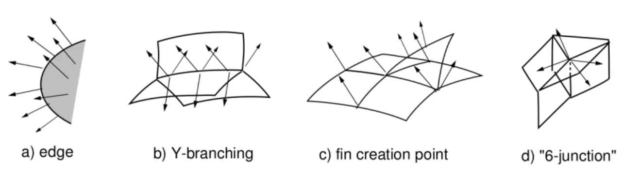
Figure 2.2. Computing integrals over regions Γ⊂Ω as medial integrals.

Given a Borel measurable function g : Ω → _R, it is possible to integrate g over a smaller region Γ ⊂ Ω, as in Figure 2.2. One must first compose g with the radial flow, compute a line integral over the portion of the radial line within Γ, then integrate the resulting function over the medial axis, as M parametrizes such lines [13]. This Crofton-type formula (Corollary 7 in [13]) is given in the next theorem.

Theorem 2.5.5. Suppose (M, U) is the Blum medial axis and radial vector field of a region Ω⊂_Rn+1_{. Let} _Γ_⊂_Ω _{be a Borel measurable region, and let} _g _{: Γ}_→

(42)

measurable and Lebesgue integrable function. If

e

gΓ(x) = Z 1

0

χΓ·g(x+tU(x))·det(I−trSrad)dt,

then _egΓ is defined for almost all x∈Mf, integrable on Mf, and

(2.15)

Z

Γ

g dV =

Z

f M

e

gΓ·r dM.

2.5.4. Examples of integration. In this section, we explicitly compute the formulas for area and volume of a region Ω in _R2 _or

R3 as integrals over M. These formulas

generalize the classical formulas of Weyl for volumes of tubes and Steiner’s formula.

Example 2.5.6 (n = 2). Suppose Ω ⊂ _R2 _{is a smooth compact region with smooth}

boundary B and Blum medial axis M. In_R2_{, the radial shape operator is simply}

multi-plication by κr, the radial curvature of M. Then the following integral is defined:

(2.16) α=

Z 1

0

det(I−trSrad)dt=

Z 1

0

(1−trκr) dt= 1− 1 2rκr. Using the above formula, we determine the area of Ω to be

area(Ω) =

Z

f M

α·r dM

=

Z

f M

r dM− 1 2

Z

f M

r2·κrdM. (2.17)

Example 2.5.7 (n = 3). As above, suppose Ω ⊂ _R3 _{is a smooth compact region with}

smooth boundary B and Blum medial axis M. Since

det(I−trSrad) = 1−tr·trace(Srad) +t2r2 ·det(Srad),

we have

α=

Z 1

0

det(I−trSrad)dt = 1−r Hrad+ 1 3r

2_K

(43)

where Hrad =

1

2trace(Srad) and Krad = det(Srad). Hence, we determine that the volume of Ω is given by the following formula:

volume(Ω) =

Z

f M

α·r dM

=

Z

f M

r dM −

Z

f M

r2·HraddM + 1 3

Z

f M

r3·KraddM. (2.18)

Remark 2.5.8. Although the medial axis is stable under sufficiently small C∞ pertur-bations of the boundary, it fails to be stable under small C1 perturbations — namely, a small change on the boundary may produce a large set-theoretic change on the medial axis. Nevertheless, area/volume undergoes only small changes under sufficiently small perturbations. In Chapter 6, we shall introduce several measures of comparison for a collection of regions which involve computing the area and volume of regions extending into the complement as medial integrals.

2.6. Medial representations in medical imaging

In this section, we describe how medial representations of a single object or region are utilized by computer scientists in the field of medical imaging. We also describe work involving multiple regions and identify a number of issues relating to multi–region analysis, both medical and mathematical in nature, that motivated the work in this dissertation.

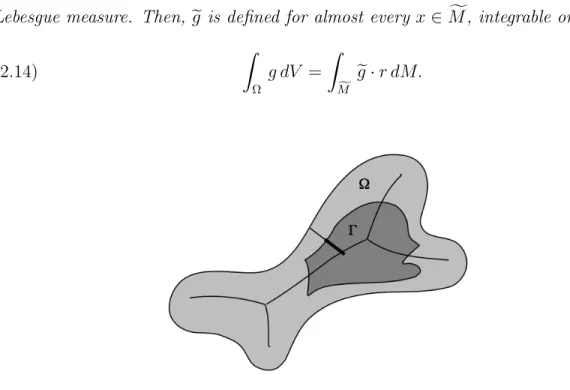
A discretized version of the Blum medial axis was introduced in [42] by Pizer, et al., who referred to it as a discrete “m-rep” or medial representation of an object. It is composed of a finite collection of medial atoms consisting of a center point and two “spokes” or radial vectors. Examples of discrete m–reps in 2 and 3 dimensions appear in Figures 2.3 and 2.4, respectively.

(44)

Figure 2.3. 2D discrete m–rep used for segmentation of the brainstem [42].

Figure 2.4. Discrete m–rep of the kidney and 3D rendering (courtesy of

Medical Image Display and Analysis Group at UNC).

(45)

Figure 2.5. Example of discrete m–reps of a complex of organs.

On the left, discrete m–reps of the prostate and bladder. On the right, bladder images produced from the m–reps demonstrating the influence of the prostate on the bladder

[26].

Pizer and other members of the Medical Image Display and Analysis Group at the University of North Carolina have begun to apply the techniques of single region medial analysis to multiple objects or regions, such as complexes of organs in the body. We now describe a number of medical and mathematical issues that arise in the context of multiple region shape analysis.

First, fundamental questions from the single region setting carry over to multi–region shape analysis, such as:

(1) How may one perform statistical analysis on images of organ complexes in order to effectively analyze the images and aid in treatment planning?

Moreover, moving from shape analysis of one object to a collection of objects involves the examination of the following:

(2) What relationships exist within a collection of objects, including any influences that objects may exert over other objects?

For example, when the bladder fills, the nearby prostate presses on it and changes its shape as illustrated in Figure 2.5.

(46)

Figure 2.6. A second example of a multi–object complex.

Image of subcortical brain structures constructed from multiple m-reps used in a study of differences in brain structures between autistic and typically developing children [24].

predict the location of the prostate. This issue brings up the following mathematical question:

(3) How may one obtain a correspondence between regions on nearby objects that should to some degree be statistically correlated based on their proximity to one another, as well as examine variations in this correspondence across populations? Presently, Pizer, et al. employ user-based identification of object or region closeness (see, e.g., [41], [30], [26]), so one objective in extending medial analysis to multiple regions is to aid in rigorizing the choice of correspondence between neighboring regions.

Another issue relates to the fact mentioned earlier that organs or portions of objects in the body may undergo shape or position changes based on the influences of other nearby organs:

(47)

scale levels, including global deformations applied to every discrete m–rep in an image to deformations within a portion of a single m–rep. This raises the question of how can one make the following notion mathematically precise:

(5) How may one study relations among objects or sections of objects at the same scale level?

(48)

CHAPTER 3

Blum Medial Linking Structure as Extension of Medial

Analysis to Multiple Regions

3.1. Introduction

In this chapter, we extend the analysis of the Blum medial axis of a single region to multiple disjoint regions by introducing theBlum medial linking structure. This structure is designed to enable us to study the geometry of a collection of regions relative to one another by capturing the relationships between their medial axes and their interactions with the exterior medial axis of the complementary region.

We begin Section 3.2 by stating our genericity assumptions and their consequences, then introduce the notion of medial linking in Section 3.3. In Section 3.4, we expand upon the classification of Mather and Yomdin described in Chapter 1 by classifying the generic forms of medial linking in 2 and 3 dimensions, deferring the proofs of the transversality theorem and transversality conditions that yield these results to Chapters 4 and 5, respectively. As a consequence of the classification theorems, we develop in Section 3.5 a fundamental component of the linking structure: labeled refinements of the Whitney stratifications of the boundaries and the medial axes to reflect interactions between regions. In Section 3.6, we define the final major piece of the linking structure, a collection of multivalued vector fields defined on the individual regions’ medial axes that satisfy certain properties in relation to other regions’ medial axes and the medial axis of the complementary region.

(49)

shall apply the linking structure to address questions of interest from the perspectives of both mathematics and medical imaging.

3.2. Genericity assumptions

We begin with some initial genericity assumptions from the single region case which we shall further supplement for the multi-region setting. Let X =

q

a

i=1

Xi, where eachXi

is a smooth,n-dimensional, compact, connected, orientable manifold. Letφ :X ,→_Rn+1

be a smooth embedding, and let φ|Xi = φi : Xi ,→ Rn+1 for i = 1, . . . , q. For each

i, let Bi = φi(Xi); by the Jordan-Brouwer Separation Theorem, Bi bounds a compact connected region in _Rn+1, which we denote by Ωi. We shall restrict our attention to the subset DEmb(X,_Rn+1₎_⊂_Emb(X,

Rn+1) of smooth embeddings satisfying the condition

that Ωi∩Ωj =∅for i6=j. We begin with a simple lemma.

Lemma 3.2.1. The set DEmb(X,_Rn+1₎ _{is an open subset of} _Emb(X,

Rn+1) in the C∞

topology.

Proof. Let φ ∈ DEmb(X,Rn+1), where φ(Xi) = Bi bounds a region Ωi for every i = 1, . . . , q, and let δ = min

i6=j d(Ωi,Ωj), where d denotes the minimum distance from Ωi to Ωj. Now, δ >0 since the Ωi are compact, pairwise disjoint, and finite in number. For any >0 and for any i= 1, . . . , q, let

Ω_i ={x∈_Rn+1 :d(x,Ωi)< }.

Assume < δ/4. Observe that, by the triangle inequality and the definition ofδ, Ω

i∩Ωj = ∅ for i 6=j. If necessary, shrink to ensure that ∂Ω

i is smooth for every i. That this is possible follows from the fact that

∂Ω_i ={x∈_Rn+1_:_d(x,_Ω

i) =}