STOCHASTIC AND SEMI-CLASSICAL APPROACHES TO THE QUANTUM VIRIAL EXPANSION
C. R. Shill
A dissertation submitted to the faculty at the University of North Carolina at Chapel Hill in partial fulfillment of the requirements for the degree of Doctor of Philosophy in the Department of Physics.
Chapel Hill 2019
c 2019 C. R. Shill
ABSTRACT
C. R. Shill: Stochastic and Semi-Classical Approaches to the Quantum Virial Expansion (Under the direction of Joaquin Drut)
TABLE OF CONTENTS
LIST OF FIGURES . . . vii
LIST OF ABBREVIATIONS AND SYMBOLS . . . ix
1 Introduction . . . 1
1.1 Background Experiment and Motivation . . . 1
1.1.1 Ultracold Atomic Gases . . . 2
2 Statistical Mechanics and Thermodynamics . . . 5
2.1 Thermodynamics . . . 5
2.2 Classical Statistical Mechanics . . . 6
2.2.1 The Ideal Gas . . . 8
2.3 The Canonical Ensemble andZ as a Path Integral . . . 12
2.3.1 An alternative expression for the partition function . . . 14
2.4 The Grand Canonical Ensemble . . . 15
2.4.1 Quantum Statistics Derivation of the Grand Canonical Ensemble . . . 16
2.4.2 The Quantum Ideal Gas . . . 22
2.4.3 Path Integral Representation ofZ . . . 24
3 Lattice Monte Carlo Methods . . . 26
3.1 Lattice Monte Carlo Method . . . 26
3.1.1 Trotter-Suzuki Factorization . . . 28
3.1.2 The Hubbard-Stratonovich Transformation . . . 28
3.1.3 Assembling the field integral representation . . . 29
3.1.4 Doing the Integral with Monte Carlo Methods . . . 30
3.2 Hybrid Monte Carlo . . . 32
3.3 The Sign Problem . . . 35
3.3.1 Complex Langevin Method . . . 36
4 Friedel Oscillations . . . 38
4.1 Introduction . . . 38
4.2 Many-body method . . . 41
4.2.1 Hamiltonian and basic formalism . . . 41
4.2.2 Expectation values of operators . . . 44
4.3 Results . . . 45
4.3.1 Ground-state energy . . . 46
4.3.2 Density profiles . . . 46
4.3.3 One-body density matrix . . . 48
4.3.4 Quasi-momentum distribution . . . 48
4.3.5 Tan’s contact density and contact . . . 49
4.4 Summary and Conclusions . . . 50
5 Virial Projection in 1D and 2D . . . 59
5.1 Introduction . . . 59
5.2 Formalism . . . 61
5.2.1 Stochastic Methods . . . 61
5.2.2 Semiclassical Lattice Approximation . . . 63
5.3 Results . . . 64
5.3.1 Virial coefficients in 1D . . . 64
5.3.2 Radius of convergence via projection method . . . 65
5.3.3 Virial coefficients in 2D . . . 65
5.3.4 Semiclassical lattice approximation . . . 66
5.4 Summary and Conclusions . . . 68
6 Systems with Three-Body Forces . . . 71
6.1 Introduction . . . 71
6.2 Hamiltonian and virial expansion . . . 71
6.3 The semiclassical approximation at leading order . . . 73
6.4 Results . . . 75
6.4.1 Virial coefficients . . . 75
6.4.2 Thermodynamics and contact across dimensions . . . 76
6.5 Summary and Conclusions . . . 77
LIST OF FIGURES
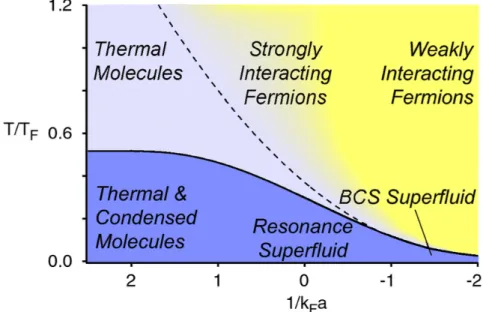
1.1 A representation for some of the possible systems of which we have access with the high degree of control of temperature (T /TF) and interaction strength (1/kFa) in 3D (13). We will discuss
some of these regimes throughout this dissertation. . . 3
3.1 Running average over Langevin time,τ, whereτ0is the total number of Langevin time steps, of
the total particle numbers,hˆn↑iandhˆn↓i. Separate runs are seen to converge to the expected particle number for the 2 + 1 case (blue) and the 6 + 3 case (red). The data corresponds to V =Nx3,Nx= 6,β= 3.0, tuned to the unitary limit. . . 33
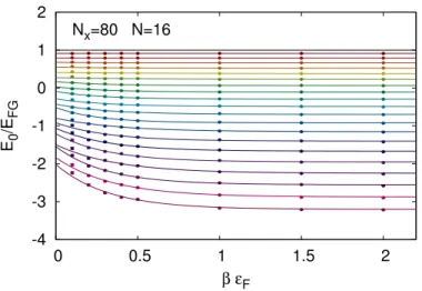
4.1 Convergence of our energy estimator as a function of βεF, for N = 16 particles in a 1D segment (discretized usingNx= 80 points), for couplingsγ= 0.0,0.2, ...,4.0 (top to bottom). 52 4.2 The ground-energy of N = 8, ...,24 unpolarized fermions in a 1D segment (discretized
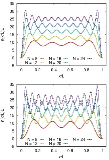
us-ing Nx = 80 points), in units of its non-interacting counterpart EFG, as a function of the dimensionless couplingγ. . . 52 4.3 Density profiles versus the scaled position x/L forNx = 80 at weak coupling (γ = 0.2, top
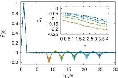
panel) and strong coupling (γ= 3.0, bottom panel), for particle numbersN= 8,12,16,20,24 (from bottom to top). . . 53 4.4 Hard-wall transform coefficientsBk of Eq. (4.34), as a function of Lpk/π =k, for Nx = 80
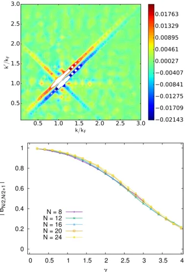
and several values of the coupling γ and particle numberN. Note the maximum at k = 1 is equal to unity to an accuracy better than 2% for all γ and N; the minima, on the other hand, show clear variation with increasingN = 8, ...,24 (left to right) as well as increasingγ (top to bottom; see inset). Inset: Value of the minimum as a function of the couplingγ for N = 8, ...,24 (bottom to top). . . 54 4.5 Top: Hard-wall transform coefficients Bk,k0 of Eq. (4.36), as a function of k = Lpk/π and
k0 =Lpk0/π, forNx = 80,γ = 4.0, and N = 24. Bottom: Amplitude variation of the main
peakBN 2,
N
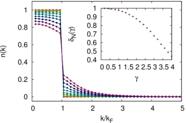
2+1 as a function ofγ for several particle numbers. . . 55 4.6 Quasi-momentum distributionn(k) forN= 16 particles as a function ofγ= 0.2,0.6,1.0, ...,3.8
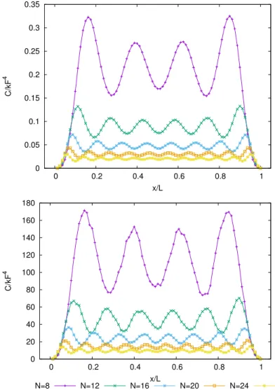
(top to bottom around k= 0), for Nx= 80. Inset: γ-dependence of the discontinuity δN in n(k) at the Fermi surface. While δN could depend on N, our results for different N agree within our statistical and systematic uncertainties. . . 56 4.7 Contact densityC(x/L) as a function of the scaled positionx/LforNx= 80 at weak coupling
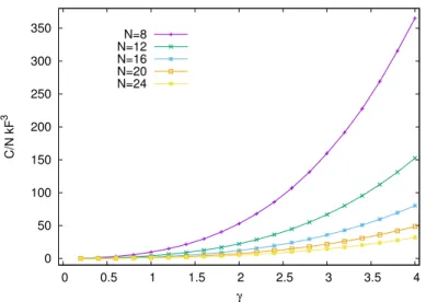
(γ = 0.2, top panel) and strong coupling (γ = 3.0, bottom panel), for particle numbers N = 8,12,16,20,24 (top to bottom). . . 57 4.8 Tan’s contact ofN = 8, ...,24 unpolarized fermions in a 1D segment (discretized usingNx= 80
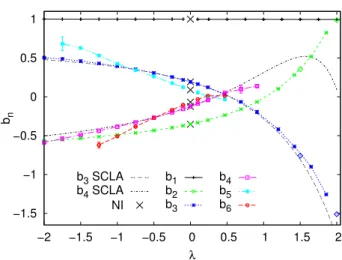
points), in units of its non-interacting counterpart EFG, as a function of the dimensionless couplingγ. . . 58 5.1 Virial coefficients bn for n = 1−6 for the 1D Fermi gas, as a function of the
dimension-less coupling λ, as obtained with our projection method. Crosses on the y axis denote the non-interacting valuesbn= (−1)n+1n−3/2. The leading order of the semiclassical lattice
ap-proximation (LO-SCLA) is shown with a dashed-dotted line for ∆b3and with a dashed line for
∆b4. Green and blue diamonds show the results obtained with our second stochastic method,
for comparison. . . 64 5.2 Estimate of the radius of convergenceα0 of the virial expansion as a function of the coupling
λ. Inset: bn forn= 1,3,5 forλ=−1. Constant behavior as a function ofαis expected when
5.3 Interaction change of the virial coefficients ∆bn for n = 2−4 for the 2D Fermi gas, as a
function of the dimensionless couplingλ2. The solid red line connects the data for ∆b2, the
green shows ∆b3, and the blue shows ∆b4. The leading order of the semiclassical lattice
approximation (LO-SCLA) is shown with a dashed-dotted line for ∆b3and with a dashed line
for ∆b4. The solid black line shows the result for ∆b3of Ref. (73). Note that the data for ∆b2
reproduces the exact result of Eq. (5.15) by virtue of the renormalization condition (see text). 69 5.4 Top: Illustration of the size of the finite-Nxeffects onb3andb4in 1D atλ= 1. The errorbars
show statistical effects. Bottom: Illustration of the size of the finite-τ effects on ∆b3 in 2D
for varyingλ. . . 70 6.1 Above are plots of the three body pressure (left) and density (right) equations of state to
order five in the virial expansion in their dimensionless form in one two and three dimensions plotted against the log of the fugacity, lnz=βµ. We have represented only one value of ∆b3
LIST OF ABBREVIATIONS AND SYMBOLS
S - Action
BCS - Bardeen Cooper Schrieffer
g - Bare Coupling
k - Boltzmann Constant
BEC - Bose-Einstein Condensate
µ - Chemical Potential
ν - Correlation Length Critical Exponent
ak(t) - Creation Operator
ak∗(t) - Annihilation Operator
Tc - Critical Temperature
Ut - Fermion Matrix
F-R - Fesbach Resonance
z - Fugacity
Z - Grand Canonical Partition Function
Ω - Grand Potential H - Hamiltonian
σ - Hubbard Stratonovich Auxiliary Field
HST - Hubbard-Stratonovich Transformation
HMC - Hybrid Monte Carlo
β - Inverse Temperature
L - Legrangian
Nτ - Number of Time Lattice Points
h - Planck’s Constant
QCD - Quantum Chromo Dynamics
QMC - Quantum Monte Carlo
SCLA - Semi-Classical Lattice Approximation
λT - Thermal Wavelength
δτ - Time Lattice Spacing
Tt - Transfer Matrix
CHAPTER 1: Introduction
Section 1.1: Background Experiment and Motivation
Throughout this dissertation, we will discuss the physics, methods, and results (computational as well as experimental) in the realm of many-body quantum systems. These systems provide an attractive playground for both experimentalists abd theorists, and is one of the most rapidly advancing areas of physics today. Since the dawn of quantum mechanics it was understood that many-body quantum systems are as important as they are challenging: indeed, calculating the properties of even small nuclei, or small electronic systems, requires considerable computational resources. For that reason, quantum many-body systems have received significant attention, leading to many fundamental discoveries both in theory and experiment. These discoveries range from measuring and studying newly discovered phase transitions, to new states of quantum matter, to even observing macroscopic quantum effects. That is, microscopic quantum effects of few particles culminate to have large effects in matter on the scale that can be seen with the human eye.
There are many examples of these types of advancements throughout the past century. One popular example is that of the observation of superfluidity in liquid4He in 1938 (4; 5), which is the phenomenon such
that liquid can flow without resistance. The trouble with this state of matter, however, is that the interaction of the molecules is so strong that the underlying physics on the microscopic level is extremely difficult to understand and model theoretically. This brings us to a great counter example, which is what occurs to non-interacting bosons when brought to zero temperature. This curiosity was first theorized by Bose long before the measurement of superfluid helium. Bose was actually able to formulate this hypothesis before, even, the final formulation of quantum mechanics, by introducing a new way of counting microstates (6). Following this discovery, Einstein generalized the technique to include particle number conservation, leading to the development of the Bose-Einstein distribution, and even more importantly Bose-Einstein condensation (BEC). This is the phenomenon whereby, at some critical temperature, Tc, bosons condense and a large
Another good example of many-body experimental development was the discovery of superconductivity in 1911 (7). Similar to superfluidity, this is when electrons can flow through a conductor without resistance. Such a surprising phenomenon was studied extensively in a large amount of different metals, as this would be an exceptionally useful tool if able to adapt for a wide variety of uses. It was not for another 50 years, however, that a group of scientists (8) discovered that this effect was actually caused by BEC. Superconductivity occurs when the electrons in a metal (as a gas of fermions) form loosely bound pairs, known as Cooper pairs, effectively forming a gas of non-interacting bosons allowing for superfluidity of the gas within the metal. Another 20 years later in 1986 the discovery of high-temperature superconductors in ceramic materials was made (4). The microscopic physics behind this, however, remain an area of hot debate to this day.
Thus far, we have discussed several important experimental and theoretical discoveries within the field of many-body quantum systems. To further our understanding of the vast advancements in this field and to understand the realm in which the majority of this work focuses, however, we must enter a slightly more specific and more modern area of quantum matter: ultra-cold atomic quantum gases.
1.1.1: Ultracold Atomic Gases
Ultracold atomic gases represent a relatively new area of study within many-body systems that came to the forefront of condensed matter research after several groups achieved BEC for the first time in a trapped dilute gas of bosonic alkali atoms in 1995 (9; 10; 11), over 70 years after its theoretical development. With this research came new techniques for studying and producing novel states of quantum matter. These techniques involve the use of 1) laser cooling, 2) trapping atoms in a magnetic trap, and finally 3) evaporative cooling (4). Those steps are essential for the observation of BEC for a few reasons. An atomic BEC first requires extremely low densities (between 1012and 1015atoms/cm3) in order to avoid crystallization of the atomic cloud; second
(and directly related to the previous item), an atomic BEC requires extremely low temperatures (1 - 100 nK). Such extremely low temperatures and densities were never before achievable through experiment. The development of magnetic trapping solved several roadblocks hindering BEC research. To begin, trapping allows experimentalists to isolate the gas from external walls, and therefore from external heat reservoirs, and impurities. Moreover, it allowed for a simple way to perform evaporative cooling. By increasing or decreasing the depth of the trap, the higher energy particles are able to escape, and scientists are able to adjust the gas to precise temperatures.
What is even more interesting is that we can utilize various numerical methods as well as advanced field theory techniques to obtain accurate microscopic depictions of these ultracold atomic systems. We will return to those later.
Our understanding of, and access to, these systems has been furthered even more so by the implementation of Fesbach-resonance techniques, F-R (12), which refers to the idea of tuning of a magnetic field about a Feshbach resonance, allowing experimentalists to precisely control interaction strength between atoms. The scattering length, and therefore interaction strength, between two particles colliding is directly dependent on the energy difference between the internal levels of the atoms. That energy difference can be controlled by tuning a magnetic field about the F-R, as the magnetic field couples to the internal properties (namely the magnetic moment) of the otherwise neutral atoms. Using the above-mentioned suite of techniques, parameters such as temperature, density, and interaction strength are under precise experimental control, giving experimentalists access to a wide array of quantum many-body systems, from weakly to strongly coupled and from nearly zero to high temperature (see e.g. Fig.??below).
Figure 1.1: A representation for some of the possible systems of which we have access with the high degree of control of temperature (T /TF) and interaction strength (1/kFa) in 3D (13). We will discuss some of these
regimes throughout this dissertation.
The ability to finely tune the interaction strength allowed for yet another huge development within this field. It allowed for the possibility of achieving superfluidity and BEC in fermions. Indeed, experimentalists were able to measure a BEC of Cooper pairs within an atomic Fermi gas (14; 15).
positive scattering length (also known as detuning), no bound molecule, weakly attractive systems (BCS), to large negative detuning where we have bound molecules. As it so happens, this transition from BCS to BEC is completely smooth, i.e. the transition is continuous (4)!
The continuation and applicability of this research is nearly limitless. For instance, all of the afore men-tioned experiments with fermions used spin 1/2 fermions (as required for poly exclusion) in an unpolarized case (n↑ = n↓). The question then is, what happens in a polarized case? A large amount of research has gone into this question that could shed light on the physics in neutron stars, where mixtures of quarks with attractive interactions exist, and could form something known as a color superconductor (4). Another outlet involves the use of lasers to form standing waves and create an optical lattice, which can be used to simulate ionic lattices, and therefore allow the study of solid state physics with the degree of control of ultracold atomic experiment. In addition, this method can even be used to provide insight into high temperature superconductors. Lastly, and directly relevant to the work in this dissertation, optical lattices can be used to create reduced dimensional systems of trapped gases. These lower dimensional systems often yield inter-esting or unexpected behaviors, such as strongly correlated effects. Crucially, when considering systems in one spatial dimension we often have the luxury of exact theoretical solutions for certain classes of systems (4).
The list of possible research directions goes on. The highly clean and controllable nature of ultracold atomic gases allows for the study of an extremely wide degree of systems, and as previously mentioned because of the nature of these systems (low density, small interaction strength) we have the capability of applying certain approximate methods to help study and explore them both theoretically and numerically on a microscopic level. This in turn allows for a high degree of collaboration between theorists and experi-mentalists, that is not usually seen in modern day physics.
CHAPTER 2: Statistical Mechanics and Thermodynamics
In this chapter we present some elementary consideration regarding thermodynamics and statistical mechanics. The goal is to introduce some of the essential quantities needed to understand the main results obtained in this thesis, which are discussed in later chapters. To that end, we begin with a review of thermodynamics in the context of classical (i.e. non-quantum) systems. We then discuss the classical ideal gas and introduce the partition function. Finally, and with a view to addressing the quantum many-body problem, we review second quantization and the quantum version of the grand-canonical ensemble.
Section 2.1: Thermodynamics
Thermodynamics studies the equilibrium behavior of macroscopic systems (macrostates), such as work heat and entropy, based on the culmination of microscopic properties (microstates) of particles, such as kinetic and potential energies and interaction strength. At the microscopic level, the physics and behavior of these particles is relatively well known through varying theories of their interactions and dynamics. Assuming these microscopic descriptions are relatively complete, we should ideally be able to describe the overarching behavior of the system, i.e. the macroscopic properties. This is best achieved using the kinetic theory of gases.
The simplest system to study to better understand this theory, is the dilute (essentially ideal) gas. Given a volume of gas,V, kinetic theory attempts to describe the macroscopic properties of the system by considering the total energy and time evolution of the N microscopic particles occupying the system. Both the energy consideration and the time evolution can be studied using the Hamiltonian,H, given the microstate of allN particles in terms of their position and momenta, q(t) and p(t) respectfully, at any time t. For this system ofN particles the Hamiltonian is defined as,
H(q,p) =
N X
i=1
p2i
2m+U(q) =
X
i
Eini (2.1)
which denotes the total energy of the system, with coordinates q ≡ {~q1, ~q2,· · · , ~qN} and momenta
p≡ {~p1, ~p2,· · · , ~pN}. Likewise, the Ei are the energy levels available to the microstates of the system, and
ni are the number of particles that occupy that energy state, such that Pini =N. Also the number of
in the 6N dimensional phase space (for 3D systems) is then governed by the canonical equations of motion,
∂~qi
∂t = ∂H ∂~pi
∂~pi
∂t = − ∂H ∂~qi
, (2.2)
These equations of motion are subject totime reversal symmetry, such that if the momenta are reversed, that isp→ −p, att= 0, the particles follow their previous trajectory,q(t) =q(−t). This comes from the invariance ofHunder the transformation (p,q)→(−p,q).
The macrostates M, of an ideal gas in equilibrium can be described by a small set of state functions like E,T, P, andN. The overall space spanned by M is much smaller than that of the space spanned by themicrostates,µ. This allows us to conclude that there must be a significant amount of microstates that correspond to a single macrostate. This is known as thedegeneracy of the system, when there are multiple sets of microstates that yield the same macrostate, and each set of these degenerate states is known as an
equivalence class (16).
Again, degeneracy is a set of microstates that corresponds to the same set state functions, and the microstates are well understood using classical physics. The question now is, how do we access the information of these macrostates? This is where statistical mechanics comes into play, which we will now discuss.
Section 2.2: Classical Statistical Mechanics
In the previous section we discussed microstates and how we can describe the corresponding macrostates by a fixed number of particles N, fixed volumeV, and a total energyH, and our set of microstates will of course be a function of these, Ω(N, V, E). This gives us a direct connection between the kinetic theory of gases and its eventual successor ensemble theory. Which reduced the problem to the overarching statistics of the problem on the whole. So we migrated from a direct application of classical mechanics to the collective statistics of the system. So inevitably this new theory became known asStatistical Mechanics, go figure.
The idea behind the statistical nature of thermodynamics comes from the fact that we consider a macrostate with a larger number of microstate a more probable one. In fact the state in which the number of microstate, Ω(E0, Ei), is maximized is considered the most probable one. This is due to the fact that
therefore can be identified as theequilibrium state. We may obtain this equilibrium state as,
∂Ω(Ei)
∂Ei
= 0, (2.3)
and the corresponding energy associated with this state is denoted ¯Ei. Furthermore the equilibrium state
can be defined by a parameter,β, which can be defined as follows,
β=
∂ln Ω(N, V, E)
∂E
N,V,E= ¯E
. (2.4)
It can also be stated that if we have multiple systems in contact corresponding to a givenNi,Vi, andEi,
then these systems are in equilibrium precisely when theβiare equal. This is because at this point there must
be no more net energy exchange between the systems (16). We can then conclude that this parameter,β, must be related the thermodynamic temperature of the system. Recall, from your introductory thermodynamics class, the following,
∂S
∂E
N,V
= 1
T, (2.5)
such thatS is the entropy of the system. From these two previous equations, we can then conclude that there is a relationship of these two of the form,
∆S ∆ ln Ω =
1
βT =C. (2.6)
This was first determined by Boltzmann, and corresponds to a universal constant. Plank then followed this with a definition for entropy in terms of the number of microstates of a system,
S=kln Ω, (2.7)
and thus provided us with a statistical connection to the third law of Thermodynamics. This relationship allows us to further develop thermodynamics, and our understanding of universal constants. Namely,
η =
∂ln Ω(N, V, E) ∂V
N,V,E= ¯V
, (2.8)
ζ =
∂ln Ω(N, V, E)
∂N
N,V,E= ¯N
.. (2.9)
state,
dE=T dS−P dV +µdN, (2.10)
where P is the thermodynamic pressure, andµthe chemical potential of the system. It follows that,
η=βP, andζ=−βµ, (2.11)
such that β = 1/kT is the inverse temperature, and k the Boltzmann constant. The same equilibrium conditions as with ¯Eapply here as well. Various other thermodynamic equations can be found in a standard Statistical mechanics book such as Pathria (16). To advance our understanding of the applications and implications of statistical mechanics, let us examine a specific system that in itself has many implications to other systems and much of our own work, theideal gas.
2.2.1: The Ideal Gas
The ideal gas is a highly specialized system, but allows us to get a straightforward understanding of the Boltzmann constant and its relationship to other physical constants. Not only does this system provide insight into natural constants, but the classical ideal gas often provides parallels to other more complex systems, particularly real gases in extreme limits. For instance, taking the limit of high temperature, weak coupling, or dilute systems often brings us back to a similar behavior of the ideal gas.
In this system we are considering a set of classical, non-interacting particles, meaning that there is no spacial correlation between the location of the individual particles and the likelihood of a given particle to be in a specific location. That is to say that the location of these particles is independent of the location of the others. This implies that the total number of ways that the N particles may arrange themselves in the given volume,V, is equal to the product of the number of ways the particles may arrange themselves in the space independent of the others. With the total number of particles N, and the total energy E fixed, this number will be directly proportional to the volume of the system. It follows that the total number of microstates is thus proportional to the Nth power of V:
Ω(N, E, V)∝VN. (2.12)
Combined with eq.(2.9) we can obtain
P T =k
∂ln Ω(N, V, E)
∂V
N,E
=kN
Which then leads to the very well known ideal gas law,
P V =kN T, or P V =nRT, (2.14)
where nis the number of moles of gas contained in the system, and R=kNA,NA being the Avogadro number. This holds for any system of non-interacting particles, or can be employed as an approximation for
nearly non-interacting systems (16).
To continue we will need to examine the relationship between the total energy and the energy of the various degrees of freedom for the system (r). That is, how many ways can we satisfy the equation,
3N X
i
i=E. (2.15)
The energy eigenvalues associated with a free system of particles confined in a three dimensional box of lengthL, such that the corresponding wave-functions,ψ(x), vanish at the boundaries is given by
(nx, ny, nz) =
h2
8mV2/3(n 2 x+n
2 y+n
2
z); nx, ny, nz={1,2,3,· · · , L}. (2.16)
Here h is Planck’s constant, andm is the mass of the particles. It follows that the number of distinct microstates for a particle of a given energyis the number of independent solutions of
(n2x+n2y+n2z) =8mV
2/3
h2 =
0. (2.17)
Let us represent this number by Ω(1, , V). It then follows that the actual desired value of Ω(N, E, V) is given by all the possible solutions of
3N X
r
nr=
8mV2/3
h2 E=E
0. (2.18)
Now before we even are able to calculate Ω(N, E, V) we can draw a very important conclusion from the above equation. That is that Ω has a explicitV andE dependence of the form (EV2/3). We can therefore
make the reduction,
S(N, E, V)≡S(N, EV2/3), (2.19)
may conclude that through an adiabatic process, meaning that bothS andN remain constant, that
C being a constant. Taking this one step further using the well known thermodynamic equations,
P =
∂S
∂V
N,E
/
∂S
∂E
N,V
=−
∂E
∂V
N,S
= 2 3
E
V. (2.21)
That is that the pressure of the ideal gas is exactly equal to two thirds of the overall energy density of the system. Interesting! What’s more, combining the previous two equations we can see that,
P V5/3=C. (2.22)
Yielding the relationship between the pressure and volume in a reversible adiabatic process (16). It is safe to say that the above three equations should hold for both Quantum and classical statistics. Notice that we have not yet done a full calculation of Ω, and yet we have been able attain a significant amount of information about the system! Lets do that now, however! Compute Ω that is.
In this calculation we make the assumption of distinguishable particles (i.e. classical), meaning that if we were to exchange to particles in the system, then we would have a distinct countable microstate. It follows that the number Ω(N, E, V) or better still ΩN(E0) is exactly equal to the number of positive-integral
lattice points on the surface of an 3N-dimensional sphere with radius√E0. Now, this number can obviously be seen as an oddly behaving function of E0, considering that the close values of E0 may yield extremely different numbers for ΩN(E0). So instead let us look at a different number, ΣN(E0), which is similar to the
above number but is defined as the number of positive-integral lattice points on and within the surface of an 3N-dimensional sphere with radius √E0. So it is the number of microstates corresponding to all energy eigenvalues less-than-or-equal-to E0, or essentially the volume of the 3N-dimensional sphere, not just the surface, also defined as Σ(N, E, V). This is a much more well behaved number with respect toE0, given by
Σ(N, E, V) = X E≤E0
Ω(N,E, V) (2.23)
or likewise,
ΣN(E0) = X
E≤E0
ΩN(E). (2.24)
With this number, at least, we can expect a somewhat of an asymptotic behavior as E0 → ∞. Much more so than Ω for sure. Both numbers, however, can give us information regarding the thermodynamics of the respective system. Again detailing the N-body problem of the ideal gas, the number ΣN(E0) should
ΣN(E0)≈ 1
2
3N π3N/2
(3N/2)!E 03N/2
. (2.25)
Or in terms ofN,V, andE,
Σ(N, V, E)≈
V
h
N(2πmE)3N/2
(3N/2)!
. (2.26)
Furthermore, by taking a logarithm and applying the approximation (Stirling’s Formula),
ln(n!)≈nlnn−n (2.27)
we obtain
ln Σ(N, V, E)≈Nln
" V h3 4πmE 3N 3/2# +3
2N. (2.28)
In order to derive the thermodynamics of a given system, we must find a way to fix the value of, or at least provide limits of the overall energy of the system. Given the erratic nature of the number Ω(E), specifying a precise energy value is not justifiable based on the physical nature of the system. In addition to this issue, we cannot make the assumption that a real world system has an exactly defined energy. This is highly idealized, and would be a rather naive assumption. Almost every real world system has some sort of contact with it’s surroundings, however small, resulting in a non-exact energy value. Instead we consider an effective range of values for the energy, with bounds [E−∆
2, E+ ∆
2], where ∆ is considered small relative
to the mean value of the energy, ∆E. The resulting number of microstates, Γ, is then given by
Γ(N, V, E; ∆)' ∂Σ(N, V, E) ∂E ∆≈
3N 2
∆
EΣ(N, V, E), (2.29)
and thus
ln Γ(N, V, E; ∆)≈Nln
" V h3 4πmE 3N 3/2# +3 2N+
ln 3N 2 + ln ∆ E . (2.30)
Now, for any system such that N 1 we know that limN→∞(lnN)/N = 0, so both terms inside the curly braces can essentially be considered negligible considering that ∆/E1 is also true for a reasonable system. Therefore, for most physical systems we have
ln Γ≈ln Σ≈Nln
" V h3 4πmE 3N 3/2# +3
We therefore arrive at the conclusion that, for most practical systems, the reasonable range allowed to the energy has little to no effect on the resulting thermodynamics of said system. Holy Cannoli! The reason behind this being that the number of microstates available increases with the energy, so even if we allow all possible energy states to be occupied, between 0 andE, it is only the small range aroundE, [E−∆
2, E+ ∆
2],
that makes the most significant contribution to this number (16). Even more, since we are most concerned with the log of this value, the width ∆ can also be ignored, and the thermodynamics of the problem can be calculated in a relatively straightforward manor!
Hurray! Statistical mechanics works! Now, by holding certain quantities constant, like T and N for an isothermal change of state, or S and N for a reversible adiabatic process, many other thermodynamic properties can be derived using the same processes as above. Let’s say we’ll leave those as an exercise for the reader, or just go check out Pathria (16).
We have certainly demonstrated how the thermodynamics of a macroscopic system can be derived from considering the multiplicity or degeneracy of the microstates involved (i.e. with the numbers Γ, Σ, and Ω). The whole understanding of any given system then relies on the asymptotic behavior of these numbers, which sadly is only realized in an extremely limited number of cases, like the ideal gas problem discussed above. So the question remains, how can we use these theories to discover the thermodynamic properties of any given system?
To that end, what we have essentially worked towards in the above section, without explicitly saying so, is the formulation of statistical mechanics in terms of the canonical ensemble, and what’s more the representation of these systems in regards tothe grand partition function,Z. Which will be discussed next.
Section 2.3: The Canonical Ensemble and Z as a Path Integral
As discussed in the previous section, with the asymptotic expressions for the numbers Ω, Σ, and Γ we may discuss the thermodynamics of any given system in a relatively straightforward way. For the vast majority of physical systems, however, computing these quantities is an extremely difficult calculation to cary out. We must then look to other methods in ensemble theory to make our lives easier.
First, lets point out that a fixed energy,E, for a real system just doesn’t seem to quite fit reality. For one, it is nearly impossible to measure the total energy of a system ofN particles, and furthermore that number is so apt to change that the measured value would very quickly become obsolete. A far more telling number to describe a system would appear to be the temperature, T. An easily measured, and more importantly
In the canonical ensemble, the energy E is variable, and can take on values from zero to infinity. We may then ask the question: what is the probability that at a given time, t, that the system is found in a state that can be characterized by the energyEi? Let’s call this probability Pi. Studying the statistics of
the canonical ensemble in a similar manner as we did with the ideal gas, we can develop the thermodynamic understanding of these systems.
Using a number of statistical considerations detailing in Pathria (16), we can conclude the following,
Pi∝exp(−βEi), (2.32)
where β = 1/kT is the inverse temperature, and k the Boltzmann constant. Normalizing the above expression we can again conclude that,
Pi=
exp(−βEi) P
iexp(−βEi)
, (2.33)
where the sum in the denominator ranges over all possible energies available to our system in question. This is known as the canonical distribution function (16), and now allows us to start taking expectation values for our system. For instance the average energy,U,
U =
P
iEiexp(−βEi) P
iexp(−βEi)
=− ∂ ∂βln
( X
i
exp(−βEi) )
. (2.34)
Here U is related to theHelmholtz free energy,A= (U−T S), such that
dA = dU−T dS−SdT =−SdT−P dV +µdN (2.35)
S = −
∂A
∂T
N,V
P =−
∂A ∂V N,T µ= ∂A ∂N V,T (2.36)
We may further this by showing that there is a simple relationship between the statistical representation and the thermodynamic one given thatβ is the inverse temperature,
βA=−ln
( X
i
exp(−βEi) )
, β=− 1
kT. (2.37)
A(N, V, T) =−kTlnQN(V, T), (2.38)
where
QN(V, T) = X
i
exp(−βEi). (2.39)
The quantityQN is an extremely important quantity in modern physics known as thepartition function.
There is a large amount of modern physics research devoted to finding both exact and approximate solutions to this very equation.
2.3.1: An alternative expression for the partition function
For the majority of physical systems, the energy levels, Er, are degenerate, meaning that any given
energy level can be occupied by a number of states, gr. We may therefor write the expression for the
partition function as,
QN(V, T) = X
i
giexp(−βEi). (2.40)
Yielding the following for the probability of a given state to have an energy value Ei,
Pi=
giexp(−βEi) P
igiexp(−βEi)
. (2.41)
It is then obvious that the probability for a given state to have one of the defined energy levels is thus proportional togi, themultiplicity. Thus we can considergi to be theweight for the corresponding energy
level. This, however, does not change our fundamental understanding of the basic relations laid out in the previous section (16).
To this point we have considered systems consisting of a discrete energy structure. In reality, however, when considering the overall size of our systems of interest, coupled with the remarkably large number of particles that we see in them (think Avogadro’s number, ∝ 1023), the energy structures are vary nearly
P(E)dE=R∞g(E) exp(−βE)dE
0 g(E) exp(−βE)dE
. (2.42)
We may now make the definition of the partition function in a continuous energy basis as,
QN(V, T) =
Z ∞
0
g(E) exp(−βE)dE, (2.43)
as well as an expression for an expectation value,hfi, for the same system as,
hfi=
R∞ 0 f(E)e
−βEg(E)dE R∞
0 e
−βEg(E)dE . (2.44)
This derivation for the expectation value of a system is quite broadly applicable. In fact, it can be applied to both systems for which quantum effects are important, as well as for those that may be treated classically(16).
We are very nearly to the point where we may begin discussing the computation of these quantities using various integration methods, such as quantum and hybrid Monte Carlo techniques, but first we must take to canonical ensemble one step further, to thegrand canonical ensemble. This is because the canonical ensembles limited capabilities becomes evident very quickly once you begin to look at broader, more general systems (16).
Section 2.4: The Grand Canonical Ensemble
As mentioned, the limited usefulness of the canonical ensemble becomes quite clear as you begin to study broadly applicable systems. The need for a more generalized approach becomes necessary. This generalization comes from the idea that the energyand the particle number are essentially never directly fixed, but are observed quantities (i.e. outputs) instead. We may therefore consider both E and N as variables in our system.
In order to formulate the generalization, one can begin in a similar way to that of the canonical ensemble, that is by examining a system in equilibrium, and considering the system with any particle number. This, in fact, results in a summation over all particle numbers to obtain the grand canonical partition function,Z,
Z(T, V, µ) = ∞
X
N=0
1 N!h3N
Z
e−β(H(ω)−µN)dω. (2.45)
andN have no dependence on the phase space, so let’s bring this factor outside of the integral by defining z= exp(βµ), which is the fugacity of our system. Equation [2.45] then becomes,
Z(T, V, z) = ∞
X
N=0
1 N!h3N
Z
zNe−βH(ω)dω. (2.46)
Now secondly notice that the expression inside of the integral looks exactly like our definition for the canonical partition function, which allows us to reduce even further,
Z(T, V, z) = ∞
X
N=0
zNQN. (2.47)
This is a very important definition that I will ask you to please keep stored away for future discussion, thank you.
The relationship between the grand canonical partition function to thermodynamics is not direct. We must first get at what we call thegrand potential, Ω, which relates toZ as follows,
Z =e−βΩ→βΩ =−lnZ =−βP V. (2.48)
Therefore,
P(z, V, T)≡ β
V lnZ(z, V, T) (2.49)
We now have access to exact thermodynamic quantities in systems with an arbitrary particle number, a much more broadly applicable representation (16). Now lastly, before we begin our discussion of integration methods, let us examine the formulation using quantum statistics.
2.4.1: Quantum Statistics Derivation of the Grand Canonical Ensemble
The previous sections involved general forms that allowed us to examine both classical and quantum systems consisting of distinguishable particles. Most physical quantum systems, however, involve indistin-guishable particles such as bosons and fermions. This is an extremely important distinction to make. We therefore must write our above derivations in a form that allows for a more natural quantum mechanical definition. That is, we will rewrite in terms of operators and wave functions. So from here on out we take quantities such as the hamiltonian to the operator form,H→Hˆ (16).
for the fluctuation of both these quantities. We will thus introduce a quantum formalism that allows for exactly this, second quantization.
Second Quantization
In order to work in a system where particle number is not fixed, we choose to work in a vector space comprised of the vacuum state,|0i, all possible single particle states,{|αi}, all two particle states,{|α1α2i},
all three particle states, and so on until we reach an infinite particle state. This set of all possible states of any particle number is known as theFock space. We may represent the Fock space in terms of single particle quantum numbers as,
∞
X
N=0 X
α1···αN
|α1α2· · ·αNihα1α2· · ·αN|= 1 (2.50)
By definition, states of different particle number are orthogonal. The question then is, how do we transition from a state of one particle number to another? For fermions, we do this with the use of creation and annihilation operators, defined as follows,
a†α|α1α2· · ·αNi=|ααα1α2· · ·αNi, (2.51)
aα|α1α2· · ·αα· · ·αNi=|α1α2· · ·αNi. (2.52)
Where aα and a†α are the adjoint to each other such that (a†α)† = aα. The creation and annihilation
operators add and subtract fermions from the currentN particle state respectively. a†α, the creation operator,
adds a particle with the quantum numberαto the existing set ofN single particle states, takingN →N+ 1. Since we are dealing with fermions, however, if the quantum state corresponding toαis already occupied, then the result is zero due to Pauli exclusion. Furthermore, notice that applying these operators may affect the ordering of the states. Reordering them may introduce a minus sign, since fermions are antisymmetric when switching particles. Similarly,aα, the annihilation operator takes N →N−1, and, when acting on
the vacuum state or a state where the quantum state corresponding toα is unoccupied, the result is zero (17).
{aα, a†β}=aαa†β+a
†
βaα=δα,β, (2.53)
{aα, aβ}={a†α, a
†
β}= 0. (2.54)
These relationships can easily be shown given the properties previously discussed.
Now that we have developed the formalism for creation and annihilation operators, we can create anti-symmetricN-particle states in a straightforward manor. That is, we can apply the creation operator to the vacuum state,
|α1α2α3· · ·αNi = a†α1|α2α3· · ·αNi=a †
α1a †
α2|α3· · ·αNi · · · = a†α1a
†
α2· · ·a †
αN|0i=
Y
i
a†αi|0i. (2.55)
Equation 2.55 allows us to create ANY vector in the Fock space of N-particle fermion systems, and what’s more, by definition this formulation adheres to the Pauli exclusion principal by the properties of the creation and annihilation operators (17).
A very similar formulation can be done for bosons as well, but without the need to enforce the Pauli principal. We mainly focus on fermions, however, so if one would like to get a better understanding of this formulation see such references as (16; 17).
To this point we have discussed how to develop the Fock space of quantum states using second quanti-zation, but what about the other operators used to develop the various theories in the various systems that these particles are occupying? Let us now discuss the other operators that may be developed using second quantization.
There are two main types of operators that we focus on in this work. Those are one, and two-body operators. There are, of course, three, four, and five-body operators, but in this work we are largely using two-body interactions. Examples of one-two-body operators are the density operator ˆn, the particle number operator
ˆ
N, and the kinetic energy operator ˆT. The density operator, which determines if the state corresponding to αis occupied, is defined as,
ˆ
such that,
ˆ
n(α)|α1α2· · ·αNi = aα†aα|α1α2· · ·αNi (2.57)
=
|ααα1α2· · ·αNi ifαis occupied.
0 ifαis not occupied.
(2.58)
This is rather straightforward to see becauseaαacting on the given state vector will only return a vector
ifαcontains a particle, it returns zero otherwise. a†α will then repopulateαwith a particle, returning the original state possibly unordered.
We can now use the density operator to create another important one-body operator, the particle number operator, ˆN. Again, this is a straightforward definition based on the properties ofa†α andaα,
ˆ N=X
α
ˆ
n(α) =X
α
a†αaα, (2.59)
such that,
ˆ
N|α1α2· · ·αNi= X
α
a†αaα|α1α2· · ·αNi=N|α1α2· · ·αNi. (2.60)
Once again, it is easy to see that this is true given the properties of the density operator above (17). We have given a fairly plain definition of these operators, that is the only distinguisher between them is the quantum numberα. This is extremely limiting as we will be dealing with particles of multiple quantum numbers (like alpha, as well as spin, among others), as well as points in space-time. The use of second quantization, however, allows for this designation to be made quite easily,
aα→asα(x, t). (2.61)
This allows for a much more comprehensive theory to be developed, while at the same time maintaining all the properties that we have previously mentioned.
ˆ
Vcontact= ˆn↑α(x, t)ˆn
↓
β(x
0, t0). (2.62)
This makes sense because this will only return some non-zero when two particles of different flavor occupy the same quantum state at the same point in space-time. This is to say,
ˆ
Vcontact|Φi = ˆn↑α(x, t)ˆn
↓
β(x
0, t0)|Φi (2.63)
= δαβδ(x−x0)δ(t−t0). (2.64)
This type of interaction is very common in our work because, again, we are deal with ultracold atomic gases, which are extremely dilute systems dominated by short-range interaction. Short-range interactions are very well duplicated by contact interactions in this theory.
We are now at a point where we can officially develop the formalism for the grand-canonical partition function in the quantum realm using second quantization.
Grand Canonical Ensemble in the Quantum Realm
Using the above development of second quantization, we can create the density operator of our entire system, ˆρ, as,
ρmn(t) =
1 N
N
X
k=1
{ak m(t)a
k∗
n (t)}. (2.65)
Such thatN is the total number of identical systems, andak
m(t) andakn∗(t) are creation and annihilation
operators respectively. Note that the diagonal elements of this matrix,ρnn, represent the probability that a
given system, at timet, is in the stateφn. Whereφn is a solution to the Schrodinger equation. So therefore
we may assume,
X
n
ρnn= 1 or trρ= 1 (2.66)
We may now define an expectation value in this system as,
hfi=
trρˆfˆ
tr( ˆρ) (2.67)
to the Hamiltonian as follows,
ˆ
ρ = X
n
|φni
1 QN(β)
e−βEnhφ
n|
= 1
QN(β)
e−βHˆX
n
|φni hφn|
= 1
QN(β)
e−βHˆ = e −βHˆ
tre−βHˆ
(2.68)
This looks very similar to that of the canonical density represented in the previous sections. That is because this coincides directly with the quantum canonical ensemble. In order to take things to the grand canonical ensemble, we again have to take into account the particle number and chemical potential, µ, in the form of the fugacity,z(16; 17).
To be more clear, in the grand canonical ensemble the density operator ρworks on theHilbert space of the system and has an undetermined number of particles. The density operator must therefore consider not only the Hamiltonian, but also the particle number operator, ˆN. We then define our density operator as,
ˆ
ρ= 1 Z(µ, V, T)e
−β( ˆH−µNˆ), (2.69)
such that
Z(µ, V, T) =X
r,s
eβ(Er−µNs)= tre−β( ˆH−µNˆ)= ∞
X
N=0
zNQN (2.70)
is of course the grand canonical partition function (16; 17).
2.4.2: The Quantum Ideal Gas
As discussed in section 2.2.1, when examining a system of classical, non-interacting particles, the ther-modynamics can be determined by considering the total number of ways in whichN particles may arrange themselves in a system of volume, V, and fixed total energy, E. That is we can determine the thermody-namics by calculating the total number of microstates. The classical prescription, however, is quite limited when considering naturally occurring systems because the classical nature of particles breaks down in many instances, such as in low temperature and high density systems. This is due to the fact the the thermal wavelength of a given particle, λT, in these regimes becomes comparable to the intra-particle spacing (i.e.
classical application only applies when the following inequality holds,λT (V /N)1/3, in 3D).
We mentioned in the introduction that this work mainly focuses on ultracold atomic gases, which is in fact very low temperature, meaning that a quantum prescription is needed. So let us again consider a system of volumeV, and energyE, and again attempt to calculate the quantity Ω(N, V, E).
Let us begin using equation 2.70:
Z(µ, V, T) =X
r,s
eβ(Er−µNs)= tre−β( ˆH−µNˆ)= ∞
X
N=0
zNQN
As mentioned, however, this equation is essentially impossible to compute directly for indistinguishable particles. The expression in terms of theQN on the other hand may be calculated. So if we wish to compute
Z and therefore Ω exactly, then we are tasked with calculatingQN for allN.
Recalling equation 2.39,
QN(V, T) = X
r
exp(−βEr),
such thatrsums over all the possible energy eigenvalues of theN particle system,Er, which may in fact be
written in terms of the single particle energy eigenvalues found from the single particle Schr¨odinger equation of the system,, such that
Er= X
n. (2.71)
Here,ndenotes the degeneracy, the total number of particles occupying the single particle energy states,
whereP
n=N. This allows us to rewrite equation 2.39 in terms of the density of states, g{n},
QN(V, T) = X
{n}
g{n}e−β
P
Here is where the quantum statistics truly comes into play. The sum is carried out over all possible distributions ofN particles and possible energies of the system that follow the allowed occupation number for each quantum state as governed by the density of states. The allowed occupation numbers for each state are defined by various quantum particle statistics, namely Bose-Einstein statistics for bosons and Fermi-Dirac statistics for fermions which are the two types of particles that we generally see in nature. These statistics are,
gb{n} = 1, (2.73)
gf{n} =
1 if alln= 0 or 1
0 otherwise.
(2.74)
What this means is that for Bose-Einstein statistics, gb, all distributions are possible and any number
of particles can occupy the same quantum state. Whereas for Fermi-Dirac statistics, gf, only one particle
is allowed per quantum state and therefore only distributions that follow this rule are allowed (gf = 0 for
any distribution where ∃ n such that n >1). Now to carry out the calculation of QN we consider the
expressions forgf andgb into equation 2.72, and attempt to carry out the sum. This gives,
QN(V, T) = X
{n}
e−βPn, (2.75)
only inserting a 1 for bosons, and restricting the sum over{n}for fermions. The problem with this expression
here is that we would be summing over all possible distributions ofN particles for all possible energy levels of the given system, which is extremely difficult. Let us instead insert this expression into equation 2.71, for theZ,
Z(z, V, T) = ∞
X
N=0 "
zNX
n
e−βPn
#
(2.76)
= ∞
X
N=0 "
X
n
Y
(ze−β)n
#
. (2.77)
Notice now the sum over both N and {n} may be reduced. Considering that the sum over {n} is
Z(z, V, T) = X
n0,n1,···
[(ze−β0)n0(ze−β1)n1...] (2.78)
= Y
(ze−β)n. (2.79)
Now this is something we can deal with! For bosons we sum each nfrom 0 to ∞, for fermions we need
only sum over 0 to 1. We now the solutions to both of these summations,
Z=
Q
1
(1−ze−β) for bosons
Q
(1 +ze
−β) for fermions.
(2.80)
This, in turn would make the grand potential, Ω,
Ω≡lnZ=∓X
ln 1∓e−β
. (2.81)
This is a reasonable expression that can be easily handled. Given that we are dealing with a non-interacting gas, then we can sum over all possible kinetic energy states given by ~2k2
2m, where we sum over
allk. This sum can be easily carried out, and thermodynamic quantities can be easily computed by taking derivatives of Ω.
Now that we have a firm understanding of the various ensembles as applied to quantum statistics, let us take the next step in the development of these theories. We have repeatedly mentioned that to actually make computations in meaningful systems then we need to be able to apply statistical integration techniques. This requires us to put these expressions into an integrable form. We will now discuss this topic.
2.4.3: Path Integral Representation ofZ
The idea of a path integral in quantum mechanics comes from the time evolution operator in quantum mechanics,U(xa, xb, t), given by,
U(xa, xb, t) =hxa|e−i ˆ Ht/~|x
bi. (2.82)
This allows us to calculate the probability that a particle will transition from state xa to xb, i.e. the
probability that the particle will follow the path fromxa toxb in a time,t. Adjusting this to path integral
U(xa, xb, t) = X
all paths
ei(phase)=
Z
Dx(t)ei(phase), (2.83)
where R
Dx(t) is a way two write ”sum over all paths”, or, say, integrate over all paths. A path integral! But what is this phase that we have mentioned? When considering the classical limit, there is only one idea of a path, and that is a path (xc) that follows the following condition,
∂
∂x(t)(S[x(t)])|cl= 0, (2.84)
where the actionS is the time integral of the systems Lagrangian,S=R
Ldt. It would therefore make sense
that the quantum realm would hold a similar parallel, and this is true up to a constant, that is as long as S~. We may therefore write the propagation probability as
U(xa, xb, t) =hxa|e−i ˆ Ht/~|x
bi= Z
Dx(t)eiS[x(t)]/~. (2.85)
The above was a discussion on how to formulate the time evolution operator (18), but a similar devel-opment can be used to show that this applies to the grand canonical ensemble as well. We can rewrite the trace formalism for the grand canonical partition function as,
Z= tre−β( ˆH−µNˆ)=
Z
Dx(t)e−βS(x), (2.86)
where againS is theaction, defined over the pathx(t) of the Legrangian,L, such that t∈ {ti, tf},
S(x) =
Z tf
ti
L(x(t))dt. (2.87)
CHAPTER 3: Lattice Monte Carlo Methods
In this chapter we discuss the details of the lattice Monte Carlo method which will be the main tool for the remainder of this thesis. The main components of the method are the Trotter-Suzuki factorization and the Hubbard-Stratonovich transformation, which are then combined to obtain a field-integral representation of the grand-canonical partition function. The calculation of such a field integral, however, requires sophisti-cated computational approaches. Here we discussed two such approaches (which are used in later chapters), namely: hybrid Monte Carlo and complex Langevin. The latter is in fact needed as some of the situations discussed in this thesis suffer from the so-called sign problem; we discuss the latter in this chapter as well.
Section 3.1: Lattice Monte Carlo Method
As mentioned above, for the vast majority of physically interesting systems we cannot computeZ or any useful observables through direct integration. In fact, beyond the ideal quantum gas (discussed above), the 1D Ising model, and the quantum harmonic oscillator we have very few exact solutions. We must therefore apply approximations like perturbation theory and the virial expansion, as well as statistical integration methods and various other numerical techniques in order to study and perform computation in the physically interesting systems. There are plenty of numerical methods that one may utilize, i.e. Green’s function Monte Carlo, no-core shell-model, coupled cluster, density functional theory, the list goes on. Not all are created equal, however, as some may be more efficient, precise, or accurate than the others. We will focus on one numerical method in particular, lattice Monte Carlo methods.
The idea behind lattice Monte Carlo is that, one, computing on the continuum is, well, really freaking hard, and two, we need to be able to put these computations on a computer. Computers require discrete, defined steps in order to run, which is why we first discretizespace-timeso that it contains a finite number of degrees of freedom. This of course brings us away from a perfect understanding of continuous space-time, but computing in that regime was the trouble in the first place. Besides, one can increase their lattice to a point such that the continuum limit is achieved (Nτ, Nx→ ∞). Where here Nτ andNx are the number
of time and space lattice points respectively. More specifically we want to get to a point where the thermal wavelength,λT =
√
2πβ, is much smaller than the width of our lattice, 1λT Nx.
hOiˆ = trhρˆOˆi=
trhe−β( ˆH−µNˆ)Oˆi trhe−β( ˆH−µNˆ)i
. (3.1)
We can also think about this another way, by inserting a source.
Z → Z[j(x)] = trhe−β( ˆH−µNˆ−X[j(x)])i (3.2) X[j(x)] =
Z
ddxj(x) ˆO(x) (3.3)
We can then write our expectation value as,
hOiˆ = 1 β
δlnZ[j(x)] δj(x)
j
→0
(3.4)
Great, we have the formulation that we so painstakingly derived in the previous chapters. Now the question or problem is, how do we discretize this formalism? Given that ˆH= ˆT+ ˆV, and
[ ˆH,Nˆ] = 0, (3.5)
[ ˆT ,Vˆ]6= 0. (3.6)
For the non-interacting case, ˆV →0, the Hamiltonian is trivial and diagonal in all N-particle subspaces. For an interacting system, however, each N must be diagonalized individually. So the dimension of the problem grows exponentially(19). We have to consider other ways of tackling this problem.
Given the commutators above, and taking a look at our equation for the expectation value for ˆO, eq.[3.1], we may notice that the meat of the problem lies in the exponential of the Hamiltonian. This is where the physics of our problem comes from. This is the portion of our formulation that we should focus our attention. Another way of putting this is that our focus should be on thetranfer matrix,
Tt=e−t ˆ
H. (3.7)
3.1.1: Trotter-Suzuki Factorization
We wish to discretize time into a number ofNτ discrete points as follows,
e−βHˆ =he−τHˆi
Nτ =TNτ
t . (3.8)
Such that β =τ Nτ. The TSF then says that we can factorize this further (20). The simplest
approxi-mation one can make would be
e−τHˆ 'e−τTˆe−τVˆ (3.9)
But the right-hand side is not a hermitian operator, unlike the left-hand side. We then turn to a symmetric factorization, namely
e−τHˆ 'e−τT /2ˆ e−τVˆe−τT /2ˆ . (3.10)
This is now a hermitian operator that may be handled using quantum dynamics and the techniques detailed above (20). This, however, is still an extremely difficult problem to tackle as is. The potential energy factor of being where the difficulties lie. Removing this factor would obviously take us back to the non-interacting case, a trivial problem. The way to tackle a fully interacting case brings us to the
Hubbard-Stratonovich transformation.
3.1.2: The Hubbard-Stratonovich Transformation
We have successfully put our expression for the transfer matrix into a more handleable form using the TSF, but now must find some way of handling the potential energy term specifically. Let’s take a look at this problem using a specific example. For the majority of the work that we have done throughout this dissertation, we use azero-range interaction. That is to say that two particles only interact if they occupy the same point in space-time. For spin 1/2 particles, this can be characterized as,
ˆ
V =−gX
j
ˆ
n↑,jnˆ↓,j, (3.11)
where ˆns,j =ψs,j† ψs,j is the density operator, and g the bare coupling that denotes the strength of the
eτ gˆn↑,jˆn↓,j = 1 +Cnˆ ↑,jnˆ↓,j
= 1
2
X
σ=±1
(1 +√Cˆn↑,jσ)(1 +
√
Cˆn↓,jσ). (3.12)
With this we have taken an extremely difficult problem, and turned it into a manageable one, by decou-pling the interaction (19).
There are several other ways of handling this transform as well, they are listed below (19),
eτ gˆn↑,jn↓ˆ ,j = 1 2
X
σ=±1
(1 +√Cˆn↑,jσ)(1 +
√
Cnˆ↓,jσ)
eτ gˆn↑,jn↓ˆ ,j = 1 2π
Z π
−π
dσ(1 + √
Cˆn↑,jsinσ)(1 +
√
Cˆn↓,jsinσ)
eτ gˆn↑,jn↓ˆ ,j = √1 2π
Z ∞
−∞
dσe−σ2/2e−σ √
C(ˆn↑,j+ˆn↓,j)
3.1.3: Assembling the field integral representation
Taking both the TSF and the HST and applying them to equation [2.86] for the trace form of Z, again using point-like interaction for spin 1/2 particles, we have
Z ≡trhe−β( ˆH−µN)ˆ i
Z= tr
" Z
Y
i
dσiT[σ] #
=
Z
DσtrT[σ]. (3.13)
Where we define the following as,
Dσ≡Y
i
dσi (3.14)
T[σ] =T↑[σ]T↓[σ] (3.15)
Ts[σ] =U1U2U3· · ·UNτ (3.16)
Ut=e−τ ˆ T /2Y
j
(1 +√Cnˆs,jσj,t)e−τ ˆ
T /2 (3.17)
possible paths forσ. Great! Now notice that we only must deal with one-body operators, so we can actually take the trace giving (19),
trT[σ] = detM↑M↓ (3.18)
3.1.4: Doing the Integral with Monte Carlo Methods
For reference, let us go back to the expression for the expectation value of a given operator in terms of a path integral over the auxiliary fieldσ, eq. 3.4,
hOiˆ = δlnZ[j] δj
j→0
= 1 Z
δZ[j] δj
j→0
= 1 Z
Z
DσP[σ] ˆO[σ]. (3.19)
Now, Monte Carlo integration is a stochastic method, i.e. it relies on random number generation in order to estimate a given quantity. Often this is done with true random number generation, for instance one can compute the value of pi,π, by generating two randomxandy coordinates within a square and determining wether that that set of coordinates lie within a circle of diameter equal to the side length of said square. Unfortunately, such an approach is not viable for the type of problems that appear in quantum many-body physics. Instead, we rely on the use of Markov chains a probability measure to guide this random number generation.
The above formalism allows us to sample our field,σ, in a region where the true expectation value of our operator, orsignal, is likely to be. Leading to faster convergence to the “correct” value and more consistent results. Assigning a measure, however, is not as easy as it may seem. If the measure and the signal do not overlap in a significant way, then this method may result in largely inaccurate or even divergent results. This is a major issue that has plagued all fields of statistical computation since their inception, known as thesignal-to-noise problem (19).
P[σ] ˆO[σ] =|P[σ]|[sgn(P[σ]) ˆO[σ]]. (3.20)
We have thus shifted the the fluctuations in the measure to the observable, but have assured a positive definite probability. As for normalization, we can generally assume this true. By design we choose a measure that is normalized, but taking a look back at eq. [3.19] and eq. [3.13], we see that the definition ofP[σ],
P[σ]≡ trT[σ]
Z , (3.21)
is in fact already normalized by the normalization factor, N=Z.
From here computing observables is a relatively straightforward process. Using various sampling tech-niques in regards to therandom walk, and applying an accept/ reject step to move along our Markov chain, and hopefully begin to converge to the accepted expectation value of the given system. The accept/ reject step of the Markov chain usually comes in the form of the Metropolis-Hastings, or simply the Metropolis algorithm,
3.1.5: The Metropolis Algorithm
The Metropolis algorithm is main workhorse of Markov chain Monte Carlo methods, because one, it is both a simple and versatile algorithm, and two, it maintains ergodicity and is stationary relative to the probability distribution. That is to say, that the algorithm allows for the transition from one state to any other possible state, and that over a long period of time all possible states are equally likely to occur (ergodic hypothesis) (21). Needless to say, this is an hugely important part to all Monte Carlo techniques. The method is carried out as follows (22),
1. Start with some arbitrary initial configuration, σ0
2. Propose a new configuration,σ1
3. Accept or reject the new configuration using the probability,p=min{1,P[σ1]/P[σ0]}
• If accepted,σ1 becomes the new configuration used
• If rejected, continue using the previous configuration and test again with a newσ2
This transition preserved the stationary probability density, ρ(σ), as long as the chain is ergodic. That is, again, as long asσi has the ability to transition to any possible point in the state space for the auxiliary
Moving on, the running average then takes the form,
hOiˆ = 1 Nσ
X
σ
ˆ
O[σ], (3.22)
and carries an uncertainty relative to the order, O 1/√Nσ
, and that should converge to the expected value over the given number of total samples, Nτ. For instance, this convergence can be seen in fig. [??],
which displays the running average for expected particle number of given systems ofn↑+n↓ particles, over Langevin time (similar to imaginary time, but will be discussed shortly).
The next logical question is, how do we propose a new configuration to the accept/ reject step? In practice there are several ways of doing this. Namely these are,
1. Individually (one-by-one, random or ordered)
2. In clusters (spread out or compact)
3. Globally
Updating locally, i.e. individually or one-by-one, works in practice, but has terrible decorrelation proper-ties. That is in the accept/ reject step, one may see a large number of rejections. Global updates, however, have excellent decorrelation. One should see acceptance at virtually all accept/ reject steps. That’s great, but it is much more difficult to implement. This method of globally updating is known as Hybrid Monte Carlo (HMC).
Section 3.2: Hybrid Monte Carlo
We want to be able to change our configuration,σi, as much as possible without obtaining some highly
improbable configuration, while maintaining ergodicity. In order to do this we must introduce an auxiliary momentum, π, effectively transforming our n-dimensional phase space into a 2n-dimensional phase space. We then shift to thecanonical probability distribution,
P[σ, π] = e −H[σ,π]
Z . (3.23)
Figure 3.1: Running average over Langevin time, τ, where τ0 is the total number of Langevin time steps,
of the total particle numbers, hˆn↑iand hˆn↓i. Separate runs are seen to converge to the expected particle number for the 2 + 1 case (blue) and the 6 + 3 case (red). The data corresponds toV =Nx3,Nx= 6,β= 3.0,