5090.pdf

(1)

Learning of Long-Run Risk in International Markets

Steven Wei Ho

A dissertation submitted to the faculty of the University of North Carolina at Chapel Hill in partial fulfillment of the requirements for the degree of Doctor of Philosophy in Business Administration (Finance) in the Department of Finance of the Kenan-Flagler Business School.

Chapel Hill 2013

Approved by:

Mariano Croce

Riccardo Colacito

Christian Lundblad

(2)

Abstract

STEVEN WEI HO: Learning of Long-Run Risk in International Markets. (Under the direction of Mariano Croce and Riccardo Colacito.)

I develop a general equilibrium model in which agents from two countries do not observe

directly the long-run growth prospects of their economies. Instead, the agents rationally

learn the hidden components through the Kalman filter applied to international consumption

data. Learning endogenously produces: (i) a rational explanation of international contagion

phenomenon, defined as changes in one country’s asset prices in response to foreign news, that

occurs in the absence of domestic news, (ii) large and time-varying international equity risk

premia, and (iii) a resolution of the forward premium anomaly, defined as the tendency of high

(3)

Dedication

I dedicate my dissertation to my family. My name He Wei, written in Chinese

charac-ters,贺威, was given by my late Grandfather, Prof. He Renlin贺仁_麟, who came from Jiangxi

Province and worked at Shanghai Normal University 上海师_范大学. My late Grandmother,

Hao Minzhuang郝敏莊, who came from Kaifeng赫舍里氏of both Manchurian and Mongolian

descent, has instilled me the importance of education since I was young. She has always

sup-ported me studying abroad despite missing me very much. She recently passed away in

Novem-ber, 2012. To my Father, He Gang贺钢of Shanghai Nanlin Normal School南林师范学校, and

to my Mother, Dr. Su Meifang苏美芳 of Shanghai Huashan Hospital, who made my journey

possible. To my maternal Grandmother Diao Suzhen 刁素贞, and my maternal

Grandfa-ther Su Yinbao 苏寅宝who, as an architectural engineer from绍兴, has served the Shanghai

Municipal Government and worked on bridge constructions.

(4)

Acknowledgments

I am grateful for all the help I have received. I thank my advisors, Mariano Croce and

Riccardo Colacito, for the mentorship that has made my dissertation possible. I am deeply

indebted to David Ravenscraft. I also thank my committee members, Christian Lundblad and

Toan Phan for providing me with valuable guidance at many occasions. Special thanks to

Alexander Arapoglou and Gregory Brown for the teaching opportunity. I am also grateful for

the help from David Dicks, Pab Jotikasthira, Robert Connolly and Paolo Fulghieri. I am also

indebted to Wayne Landsman and Jennifer Conrad for supporting the doctoral program at

(5)

Preface

With this dissertation, I will go back to China in 2013.

(6)

List of Tables

1 Parameters used for Calibration . . . 51

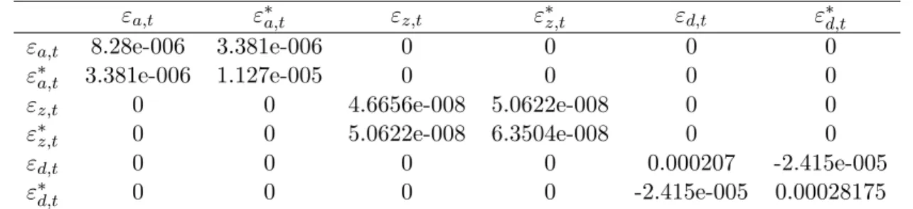
2 Variance-Covariance Matrix under Full Information . . . 51

3 True Correlation Matrix under Full Information . . . 51

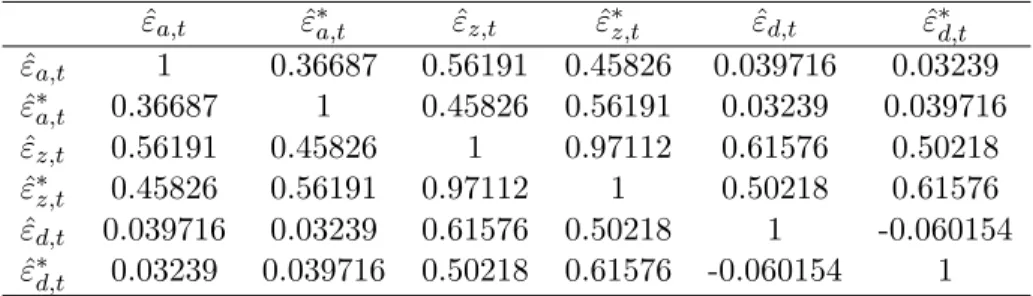
4 Correlation Matrix for Mapped Shocks under Learning from Consumption . . . 52

5 Correlation Matrix for Mapped Shocks under Learning from Consumption and Dividend . . . 52

6 Numerical value of steady-state Kalman Gain Matrix under Learning from Con-sumption . . . 52

7 Numerical value of steady-state Kalman Gain Matrix under Learning from Con-sumption and Dividend . . . 52

8 Numerical value of steady-state Covariance matrix of the filtering errors under Learning from Consumption . . . 52

9 Numerical value of steady-state Covariance matrix of the filtering errors under Learning from Consumption and Dividend . . . 52

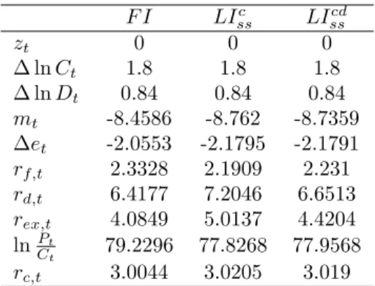
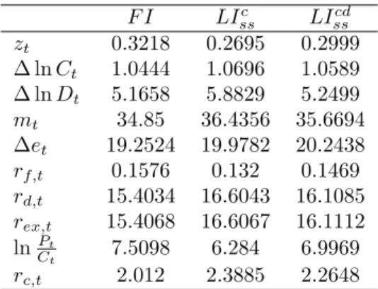
10 Numerical Simulation Results: Annualized Mean . . . 53

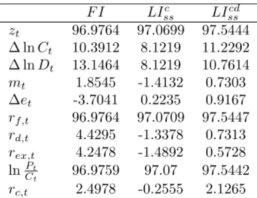
11 Numerical Simulation Results: Annualized Volatility . . . 54

12 Numerical Simulation Results: Autocorrelation-ACF(1) . . . 55

13 Numerical Simulation Results: Correlation of Home/Foreign Counterparts . . . 56

(9)

List of Figures

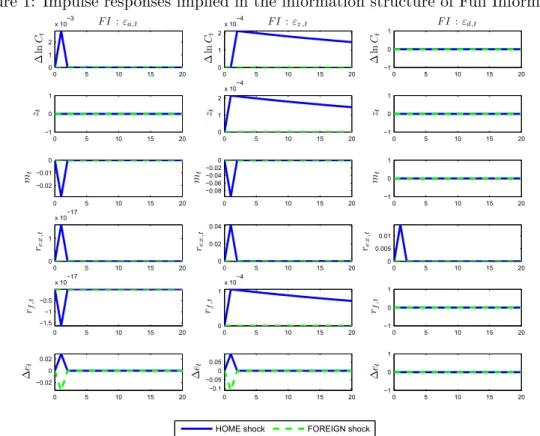
1 Impulse responses implied in the information structure of Full Information . . . 46

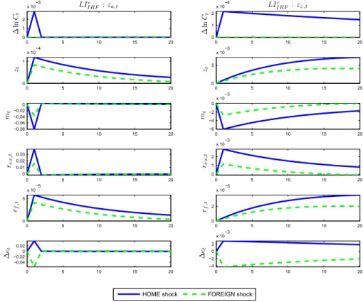
2 Impulse responses implied in the information structure of Learning from Con-sumption . . . 47

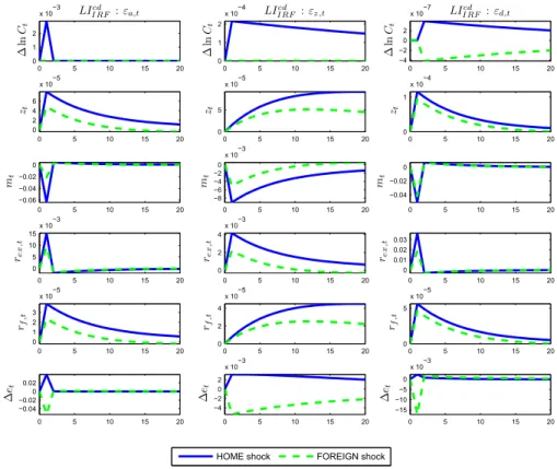
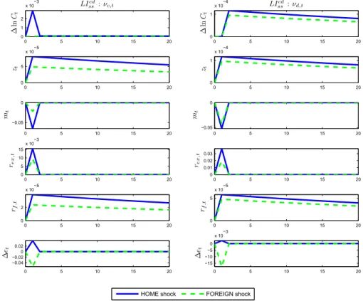
3 Impulse responses implied in the information structure of Learning from Con-sumption and Dividend . . . 48

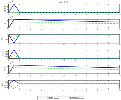
4 Impulse responses to innovation shocks implied in the information structure of Learning from Consumption . . . 49

(10)

Chapter 1 Introduction

Do agents know the long-run prospect of the economy? I address this question by

in-vestigating the international asset pricing implications of an economy in which agents have

to learn the long-run prospect of the economy from international historical growth data. To

quote from Hansen, Heaton, and Li (2008), “many of the statistical challenges that plague

econometricians presumably also plague market participants. Naive application of rational

ex-pectations equilibrium concepts may endow investors with too much knowledge about future

growth prospects”.

A growing body of the literature has documented that long-run growth prospects influence

both domestic (Bansal and Yaron, 2004) and international asset prices (Colacito and Croce,

2011). All these models are built around the assumption that consumption is exposed to two

sources of shocks perfectly observable to the agents. Specifically, short-run risk is modeled as

an i.i.d shock that only affects the economy for one period, whereas long-run risk is modeled as

a small, but highly persistent autoregressive process, which is thus expected to affect long-run

growth rates. A key question within the long-run risk paradigm is the ability of agents to

perfectly detect such a small long-run component.

Earlier papers have investigated this question in a one-country setting (Ai, 2010; Bansal

and Shaliastovich, 2011; Croce, Lettau, and Ludvigson, 2012; Johannes, Lochstoer, and Mou,

2010). In this article, I study a two-country economy, each populated by one consumer. The

(11)

risks. The agents do not know the actual value of each country’s specific long-run risk, in the

sense that they cannot can accurately break down consumption news into a component which

is going to affect the economy for many periods, and a component which represent short-run

i.i.d shocks that is only going to affect the consumption stream for one period. The long-run

components of the two countries are correlated (Colacito and Croce, 2011), thus innovation in

one country can provide information regarding the long-run component of the other country.

The Bayesian learning mechanism employed in this article is the Kalman filter (Kalman

and Bucy, 1961; Kalman, 1960). Due to the recursive nature of the Kalman filter, it can

also be viewed as the simplest dynamic Bayesian Network (Haykin, 2001; Murphy, 2002).

An intuitive interpretation of the Kalman filter approach is that in each period the agent

forms a prior regarding the joint probability distribution of the two latent variables, which

are the home and foreign long-run risks, and come up with a prediction for the following

period; as time goes by these predictions are compared with the realized observations. The

agent adjusts the estimates of the latent variables and turns her posterior distribution into a

new prior to be used in the subsequent period. Under such a setup, agent from one country

would recursively Bayesian update her estimate of her country-specific long-run component

by utilizing all available historical information in consumption growth in both countries, and

optimizes her asset pricing decisions accordingly. As an extension of the setup, I also investigate

the case of learning from both consumption and dividend stream.

I find that learning can account for prominent features of domestic and international

finan-cial markets. Specifically, the learning model presented in this article offers a solution of the

puzzling contagion phenomenon in the context of a dynamic stochastic equilibrium framework

with complete markets and no arbitrage. Contagion is broadly defined as the propagation of

shocks in excess of what can be explained by fundamentals (Forbes and Rigobon, 2000). There

is no universally accepted explanation for why contagion occurs in equilibrium (Bekaert and

Harvey, 2003; Karolyi and Stulz, 1996). This phenomenon is puzzling as one could potentially

(12)

sentiments” (Fromlet, 2001). However, such psychological arguments do not prevent an agent,

who is perfectly rational and unmoved by sentiments, from undertaking arbitrage. I propose

a rational expectations explanation for why contagion may occur in equilibrium.

I define the true long-run components of each country as the economic fundamentals, which

are unobservable and thus have to be learned, taking the history of the consumption stream

of both countries as observables. The agents of the two countries are endowed with the same

information. When agents learn using Kalman filter, they form an estimate of the entire joint

distribution of the two latent variables characterized by the means and the variance-covariance

matrix. As a result, innovations in consumption streams of both countries, are two sources of

information that will be incorporated into the estimate of the long-run persistent component

of either one country. Since the growth rates of consumption and their long-run components

are correlated across countries, the estimate of home’s economic fundamental will be revised

in response to foreign innovations, even in the absence of any new piece of information in

the home country. Equivalently, Bayesian learning gives rise to contagion as one country

may revise its long-run growth expectations solely in response to news coming from abroad.

Note that at each point in time, equilibrium prices are determined using agents’ estimates of

the distribution of fundamentals given all historical information up to that point. This means

that an econometrician who observes the entire data series may observe temporary mis-pricing,

conditional on her information set which is larger than the agents’.

The model is also able to provide a rational explanation for the forward premium anomaly,

i.e. the well-documented tendency of high interest rate currencies to appreciate (Fama, 1984),

which is at odds with the prediction of the uncovered interest rate parity relationship. The

model in this article can provide a solution due to its ability to endogenously generate

time-varying volatility through learning. Take for example the case in which the home country agent

believes that the estimate of her long-run component is very unreliable, i.e. it features a large

variance. This variance of the estimation error will steadily decrease through learning in the

transition toward the steady-state Kalman filter value. During this process, the consumption

(13)

relatively larger. By no arbitrage, the currency of the home country become more valuable,

being associated to a safer consumption profile, and it is thus expected to appreciate, despite

its higher interest rate.

Furthermore, I show that within each country, learning increases the equity risk premium

by as much as 22%. This finding confirms and extends the analysis of Croce, Lettau, and

Ludvigson (2012) to the case in which investors exploit the cross-sectional dimension of

coun-tries in addition to the domestic time-series of consumption. Additionally, when the Kalman

filter is off steady-state, the model endogenously generates time-varying uncertainty, as the

recursive application of the Bayesian updating changes the accuracy of the estimated long-run

risks through time. This means that the model features a time-varying risk-premium.

The rest of the article is organized as follows. Chapter 2 reviews the related literature. In

Chapter 3, I describe the model setup, the information structure involved, and the learning. In

Chapter 4, I present detailed derivations. In Chapter 5, I present the analytical asset pricing

solutions of learning under different information structures. In Chapter 6, I provide both

the theoretical arguments and numerical simulation results which would explain contagion in

(14)

Chapter 2 Background Literature

In the Bansal and Yaron (2004) model, there is a small but highly persistent predictable

long-run component in consumption growth, which is subject to long-run shocks. They are

called long-run shocks since due to the highly persistent nature of the long-run component,

even small innovations in this component will induce large cash flow movements in a long

time horizon. Thus, the low-frequency movements in consumption growth rates are called the

long-run risk (Bansal, Kiku, and Yaron, 2010).

A notable ingredient of the long-run risk literature, which I also employ here, is the

Epstein-Zin-Weil preference (Epstein and Zin, 1989; Weil, 1989). Under this recursive preference, agents

in each period would optimize the tradeoff between utility of current period and continuation

utility derived from all future periods (Backus, Routledge, and Zin, 2005). The recursive

preference allows the separation of coefficient of relative risk aversion γ and intertemporal

elasticity of substitution (IES) ψ, which can be simultaneously large, whereas in standard

CRRA preference ψ = 1/γ. This feature is desirable as an individual’s willingness to take

financial risk, does not have to be necessarily associated with the inverse of her inclination to

substitute today’s consumption with future consumption in response to change in intertemporal

prices (Chen, Favilukis, and Ludvigson, 2011). When IES is larger than 1/γ, agents prefer

early resolution of uncertainty and exposure to the long-run risk carries high risk premium.

Hansen and Sargent (2010) consider the model in which agents are concerned with model

(15)

agent will also update model-mixing probability and decide which sub-model is the most likely.

This setup generates elevated risk premium since agent’s distrust of her model adds to the price

of risk.

Croce, Lettau, and Ludvigson (2012) investigates the role of information in consumption

based long-run risk model and is able to explain the downward slope of equity term structure.

When investors can identify both the short-run and long-run components of consumption risk,

the standard long-run risk model can generate a sizable equity market risk premium only if the

equity term structure slopes up. However, when investors cannot distinguish short-run and

long-run components of consumption risk, the model is able to generate both a large equity

market risk premium and a downward sloping equity term structure, which is what we observe

in data.

Bansal and Shaliastovich (2011) focuses on the endogenous choice in learning. The agents

may either pay a cost to learn the true long-run component or use Kalman filtering based

on historical data. The actions of investors to learn about the true state can explain the

asset-price jumps. The model implies income volatility can predict future jumps in returns.

Ai (2010) studies the implication of public information quality about persistent productivity

shocks in a model with Kreps-Porteus preferences. The production-based long-run risk model

with learning implies that when information quality is low equity premium is high and volatility

(16)

Chapter 3 Model Setup

3.1 Preferences

There are two countries in the economy which are denoted home and foreign. Markets are

complete. As in Colacito and Croce (2011), perfect home bias is imposed in the setup so that

representative agent of each country would only consume the goods that she is endowed with.

Since markets are complete, agents can still trade Arrow-Debreu securities and they have no

home bias over financial assets. The first order conditions with respect to the purchase of

those financial assets (No-Arbitrage equations) pin down the value of all assets and the growth

rate of the exchange rate. For compactness of representation, only home’s preferences and

prices are characterized in this section. The foreign counterparts are denoted with identical

expression with a superscript “*” added to designate the variables as foreign.

Following the long-run risk literature which emphasizes the importance of long-run

eco-nomic growth prospects (Bansal and Yaron, 2004), the home representative agent has the

Epstein-Zin-Weil (1989) preference:

Ut=

(

(1−δ)C1−

1

ψ

t +δ

Et

h

U_t+11−γi

1−1/ψ

1−γ

)

1 1−1/ψ

A noteworthy feature of the Epstein-Zin-Weil preference is the separation of the coefficient

of intertemporal elasticity of substitution (IES)ψand the coefficient of relative risk aversionγ

(17)

When IES > 1/γ, agents prefer early resolution of uncertainty(Epstein and Zin, 1991). For

convenience, we can define composite parameter θ = _1−1/ψ1−γ . Denote the ex-dividend price

dividend ratio of an asset that pays a consumption stream Ct at end of period t as Wc,t =

PC

t /Ct. Also denote the ex-dividend price dividend ratio of an asset that pays a consumption

stream Dt at end of period t as Wd,t = PtD/Dt. Mt+1 is the pricing kernel and Rf,t is the

return on a one-period risk-free asset at time t. Given the Epstein-Zin-Weil preference, the

optimal consumption choice yields the following asset pricing equations:

Et[Mt+1Rc,t+1] = 1 Rc,t+1 = (Pt+1C +Ct+1)/PtC (3.1)

Et[Mt+1Rd,t+1] = 1 Rd,t+1 = (Pt+1D +Dt+1)/PtD

Mt+1 = δ

Ct+1

Ct

−1/ψ!θ

Rθ−1_c,t+1 (3.2)

Rf,t= (Et[Mt+1])−1

One can show the log pricing kernel is a function of log consumption growth ∆ct, and the

log return on an asset which pays the consumption stream rc,t+1:

(3.3)

mt+1=

1−γ

1−1/ψlogδ−

1−γ

ψ−1∆ct+1+

1/ψ−γ

1−1/ψrc,t+1

The Epstein-Zin-Weil preference and its basic asset pricing implications are shared by the

three information structures describe below.

3.2 Full Information

Let the lower-case letters denote the variables in logarithms. The processes for log

(18)

∆ct=µ+zt+σc,h·εc,t (3.4)

∆c∗_t =µ+z_t∗+σc,f ·ε∗c,t

zt=ρ·zt−1+σz,h·εz,t

z_t∗=ρ·zt−1∗ +σz,f ·ε∗z,t

∆dt=µd+λ·zt+σd,h·εd,t

∆d∗_t =µd+λ·z∗t +σd,f ·ε∗d,t

(εc,t, ε∗c,t, εz,t, ε∗z,t, εd,t, ε∗d,t)∼N.i.i.d(0,Ωc)

Ωc=



              

1 ρc 0 0 0 0

ρc 1 0 0 0 0

0 0 1 ρz 0 0

0 0 ρz 1 0 0

0 0 0 0 1 ρd

0 0 0 0 ρd 1



              

The small persistent predictable components zt, zt∗ capture the small but persistent

com-ponent of expected consumption and dividend growth rate in home and foreign countries,

respectively. Note the timing convention here is that the predictive component zt enters the

consumption growth at time t rather than time t+1. In Bansal and Yaron (2004), zt is the

conditional expectation of consumption of next period, whereas in this timing convention the

conditional expectation of consumption of next period isρzt. Letεc,t, ε∗c,tdenote the short-run

shocks to home and foreign consumption. εz,t, ε∗z,t are the long-run shocks to the highly

per-sistent component. They are called the long-run shocks because due to the highly perper-sistent

nature of zt, even a small innovation can impact cash flows for a very long time and thus

agents demand a high risk premia for the long-run shocks when IES >1/γ. εd,t, ε∗_d,t are the

(19)

Yaron (2004), dividend is not exposed to short-run shock. Indeed, for the short-run, long-run,

dividend shocks within one country,εc,t, εz,t, εd,t, each type of shock is orthogonal to any other

type of shock. On the other hand, the cross-country correlations short-run, long-run, dividend

shocks are denoted as ρc, ρz,and ρd, respectively.

In the full information case, agents observe all variables of interest and fully take equation

3.4 into account when making asset pricing decisions.

3.3 Limited Information-Learning from Consumption

Under the information structure of limited information with learning from consumption

stream, agents are assumed to observe all historical data of consumption growth, however

the agents do not observe the underlying long-run persistent components zt and zt∗. As a

consequence of limited information, the agents do not know if the innovation in consumption

is due to εc,t or εz,t. Because the linear state space of equation 3.4 is jointly Gaussian, the

agents can use the Kalman filter (Harvey, 1989) to infer the underlying latent variables, namely

zt and z∗t. The Kalman filter is the optimal linear filter for Gaussian systems. Due to the

recursive nature of the Kalman filter, it can also be viewed as the simplest dynamic Bayesian

Network (Haykin, 2001; Murphy, 2002).

Under this information structure the agent is only learning from consumption stream but

not dividend stream, the case of learning from both consumption and dividend stream would

be investigated in the next section. It would still be interesting to price dividend under the

current scenario, however, a question arises as to how to specify the exogenous dividend growth

process. Suppose the dividend process is as in equation 3.4, then the agent must be able to

infer the latent variables not only from the consumption stream, but also the dividend stream

which contains additional information regarding true values of the latent variables. In order

to achieve internal consistency with the information structure, dividend processes equation 3.4

(20)

∆dt=µd+λ·(∆ct−µ) (3.5)

∆d∗_t =µd+λ·(∆c∗t −µ)

The setup of the exogenous endowment processes are otherwise identical to the full

in-formation case. Note that the dividend process does not add any additional inin-formation for

the filtering as it is a linear transformation of the consumption process, thus the agent only

updates the filtered latent variable in response to consumption innovation.

As in Bansal and Shaliastovich (2011), I assume that Ωcis known by the agent. In addition

to knowledge about the structure of cash flow processes, agents of both countries share the

same information set at time t which is:

I_tc=

{∆ct−i}i=0,1,...,

∆c∗t−i i=0,1,...,Ωc

Note that Ωc is not time-varying. In fact, learning with off-steady-state Kalman filter can

generate endogenous time-varying volatility; more details on this and the Forward Premium

Anomaly can be found in section 6.2.

Let the filtered state vector for the case of learning from consumption stream be denoted

by z_bt,zb_t∗

b

zt=Et[zt|Itc] (3.6)

b

z∗_t =Et[z∗t|Itc]

The variance covariance matrix of the filtering errors is:

P_tc=



 

P hhc

t P hftc

P hfc

t P f fct



(21)

P hhc_t =Et[(zt−zbt)

2_|_Ic

t] (3.7)

P hf_tc=Et[(zt−zbt)(z

∗

t −zb_t∗)|I_tc]

P f f_tc=Et[(zt∗−zb∗_t)2|I_tc]

Given the filtered latent variables, the structure of the cash flow process implies the

fol-lowing innovation representation:

∆ct=µ+zbt+νc,t (3.8)

∆c∗_t =µ+zb∗_t +ν_c,t∗

∆dt=µd+λ·(∆ct−µ)

∆d∗_t =µd+λ·(∆c∗t −µ)

where the innovations in consumption in home and foreign countries are defined as:

(3.9)

   

  

νc,t=σc,h·εc,t+zt−zbt

ν∗

c,t=σc,f ·ε∗c,t+zt∗−zb_t∗

The filtering problem and its solutions are solved in section 4.1.

3.4 Limited Information-Learning from Consumption and

Div-idend

The setup of the exogenous endowment processes are identical to the full information case.

(22)

∆dt=µd+λ·zt+σd,h·εd,t (3.10)

Both the consumption process and the dividend process provide information for the filtering

of the state vector. The agents use Kalman filter to update the filtered latent variables in

response to both consumption innovation and dividend innovation. Agents of both countries

share the same information set at time t which is:

(3.11)

I_td=

{∆ct−i}i=0,1,...,

∆c∗t−i i=0,1,...,{∆dt−i}i=0,1,...,

∆d∗t−i i=0,1,...,Ωc

Let the filtered state vector for the case of learning from both consumption and dividend

stream be denoted by zet,ze

∗ t

e

zt,=Et[zt|Itd] (3.12)

e z∗

t =Et[zt∗|Itd]

P_td=



 

P hhd

t P hftd

P hfd

t P f fcdt



 

P hhd_t =Et[(zt−zet)

2_|_Id

t] (3.13)

P hf_td=Et[(zt−zet)(z

∗

t −ze_t∗)|I_td]

P f f_td=Et[(zt∗−ze∗_t)2|I_td]

Given the filtered latent variables, the structure of the cash flow process implies the

(23)

∆ct=µ+zet+νc,t (3.14)

∆c∗_t =µ+ze_t∗+ν_c,t∗

∆dt=µd+λ·zet+νd,t

∆d∗_t =µd+λ·ze_t∗+ν_d,t∗

where the innovations in consumption and dividend, in home and foreign countries are

defined as:

(3.15)

           

          

νc,t=σc,h·εc,t+zt−zet

ν_c,t∗ =σc,f ·εc,t∗ +zt∗−ze_t∗

νd,t=σd,h·εd,t+λ·(zt−zet)

ν∗

d,t=σd,f ·ε∗d,t+λ·

z∗

t −ze_t∗

(24)

Chapter 4 Derivations

4.1 Kalman Filter Derivation-Learning from Consumption

The consumption and dividend processes are assumed to be the following:

∆c∗_t =µ+z_t∗+σc,f·ε∗c,t

zt=ρ·zt−1+σz,h·εz,t (4.2)

z_t∗ =ρ·zt−1∗ +σz,f ·ε∗z,t (4.3)

∆dt=µd+λ·(zt+σc,h·εc,t)

∆d∗_t =µd+λ· z∗t +σc,f ·ε∗c,t

V ar 

       

σc,h·εc,t

σc,f ·ε∗c,t

σz,h·εz,t

σz,f ·ε∗z,t



       

=



       

σ2

c,h ρc·σc,hσc,f 0 0

ρc·σc,hσc,f σc,f2 0 0

0 0 σ2

z,h ρz·σz,hσz,f

0 0 ρz·σz,hσz,f σ2_z,f



       

(25)

Ac=    ρ 0 0 ρ    H c₌    1 0 0 1   

Qc₌



 

σ2

c,h ρc·σc,hσc,f

ρc·σc,hσc,f σ2c,f

   R c₌    σ2

z,h ρz·σz,hσz,f

ρz·σz,hσz,f σ2z,f



 

The state vector is (zt, z∗t), and the measurement vector is (∆ct,∆c∗t). In addition, the

filtered state vector for the case of learning from consumption process is (zbt,zb

∗ t).

P_tc=

        

P hhc

t P hftc

P hfc

t P f fct

        

Then by applying the standard Kalman filter update equation

P_tc=AcP_t−1c Ac0 −AcP_t−1c Hc0[HcP_t−1c Hc0 +Rc]−1HcP_t−1c Ac0 +Qc

One can show the one-step-ahead evolution equations for the variances of the filtering errors

are:

P hhct

= ρ

2_σ

c,h2 P hhct−1 −ρc2σc,f2+P f ftc−1+σc,f2

−P hfc

t−1

2

σc,f2 −ρc2σc,h2+P hhct−1+σc,h2

−2ρcP hftc−1σc,hσc,f+P f ftc−1 P hhct−1+σc,h2

−P hfc

t−1

2+σz,h

2

(4.4)

P hftc=

ρ2_σ

c,hσc,f ρc2−1

P hfc

t−1σc,hσc,f+ρc P hftc−12−P f ftc−1P hhct−1

−σc,f2 −ρc2σc,h2+P hhct−1+σc,h2

+ 2ρcP hftc−1σc,hσc,f−P f ftc−1 P hhct−1+σc,h2

+P hfc

t−1

2

+ρzσz,fσz,h

(4.5)

P f fct=

ρ2σc,f2 ρc2−1

P f ftc−1σc,h2−P f ftc−1P hhct−1+P hftc−12

−σc,f2 −ρc2σc,h2+P hhct−1+σc,h2+ 2ρcP hftc−1σc,hσc,f−P f ftc−1 P hhct−1+σc,h2+P hftc−1

2

+σz,f2

(26)

K_,tc =



 

Kc

11,t K12,tc

Kc

21,t K22,tc



 

where

K_11,tc = P hf c

t−1(−P hft−1c −ρcσc,hσc,f)

+ P hhc

t−1 σc,f2+P f ft−1c

σc,h2+P hhct−1

σc,f2+P f ft−1c

−(P hfc

t−1+ρcσc,hσc,f)2

(4.7)

K_12,tc = P hf c

t−1 σc,h2+P hhct−1

+ P hhc

σc,h2+P hhct−1

σc,f2+P f ft−1c

−(P hfc

(4.8)

K_21,tc = P f f c

+ P hfc

σc,h2+P hhct−1

σc,f2+P f ft−1c

−(P hfc

(4.9)

K_22,tc = P f f c

+ P hfc

σc,h2+P hhct−1

σc,f2+P f ft−1c

−(P hfc

(4.10)

Or, in the innovation presentation, let νLC,t =



 

νc,t

ν_c,t∗ 

 

The innovations in consumption in home and foreign countries are defined as:

(4.11)       

νc,t=σc,h·εc,t+zt−zbt

ν_c,t∗ =σc,f ·εc,t∗ +zt∗−zb_t∗

We have,

∆c∗_t =µ+zb∗_t +ν_c,t∗ (4.13)

∆dt=µd+λ·(∆ct−µ) (4.14)

(27)

And the one-step-ahead state evolution equations for the filtered home and foreign long-run

persistent components are:

b

zt=ρ·zdt−1+K

c

11,t·νc,t+K12,tc ·νc,t∗ (4.16)

b

z∗_t =ρ·zd_t−1∗ +K_21,tc ·ν_c,t+K_22,tc ·ν_c,t∗ (4.17)

The steady state Kalman filter is the solution to the following Discrete Algebraic Riccati

Equation:

(4.18)

Ac_.Pc ss.Ac

T

−Ac_.Pc

ss.Hc

T

.hHc_.Pc ss.Hc

T

+Rci−1_.Hc_.Pc ss.Ac

(28)

4.2 Kalman Filter Derivation-Learning from Consumption and

Dividend

The consumption and dividend processes are assumed to be the following:

∆c∗_t =µ+z_t∗+σc,f ·ε∗c,t

zt=ρ·zt−1+σz,h·εz,t

z_t∗=ρ·zt−1∗ +σz,f ·ε∗z,t

∆dt=µd+λ·zt+σd,h·εd,t

Ω =V ar



   

σc,h·εc,t

σc,f·ε∗c,t

σz,h·εz,t

σz,f·ε∗z,t

σd,h·εd,t

σd,f·ε∗d,t 

   

=



      

σ2

c,h ρcσc,hσc,f 0 0 0 0

ρcσc,hσc,f σc,f2 0 0 0 0 0 0 σ2

z,h ρzσz,hσz,f 0 0 0 0 ρzσz,hσz,f σ2z,f 0 0

0 0 0 0 σ2

d,h ρdσd,hσd,f 0 0 0 0 ρdσd,hσd,f σd,f2



      

Define:

Ad=h ρ₀ 0_ρ i Hd= "

1 0 0 1

λ 0 0 λ

#

Qd=

σ2

c,h ρc·σc,hσc,f

ρc·σc,hσc,f σ2c,f

Rd= 

  

σ2

z,h ρz·σz,hσz,f 0 0

ρz·σz,hσz,f σ2z,f 0 0

0 0 σ2

z,h ρz·σz,hσz,f 0 0 ρz·σz,hσz,f σz,f2



  

The state vector is _zzt∗ t

(29)

The measurement vector is 

 ∆ct ∆c∗ t ∆dt ∆d∗ t

 .

The filtered state vector for the case of learning from both consumption and dividend processes is e zt e z∗ t

. Both the consumption process and the dividend process provide information for the filtering

of the state vector.

P_td=

        

P hhd

t P hftd

P hfd

t P f fcdt

        

Then by applying the standard Kalman filter update equation

P_td=AdP_t−1d Ad0−AdP_t−1d Hd0[HdP_t−1d Hd0+Rd]−1HdP_t−1d Ad0+Qd

One can show the one-step-ahead evolution equations for the variances of the filtering errors

are:

P hhdt =

h P f ftd−1

P hhdt−1ρ 2

σd,h2σc,h2 − ρc2−1λ2σc,f2− ρd2−1σd,f2

+σz,h2λ2

σd,h2σc,f2

−ρc2σc,h2+P hhdt−1+σc,h2

−2ρcρdP hhdt−1σd,fσd,hσc,hσc,f+P hhdt−1σd,f2σc,h2

+σz,h2

− ρc2−1

λ4P hhdt−1σc,h2σc,f2− ρd2−1

σd,f2σd,h2

P hhdt−1+σc,h2

+P hftd−1 2

ρ2σd,h2σc,h2 ρc2−1

λ2σc,f2+ ρd2−1

σd,f2

+σz,h2 ρc2−1

λ4σc,h2σc,f2−λ2 −2ρcρdσd,fσd,hσc,hσc,f+σd,f2σc,h2+σd,h2σc,f2

+ ρd2−1

σd,f2σd,h2

+ 2P hftd−1σd,fσd,hσc,hσc,fσz,h2 ρc2−1

ρdλ2σc,hσc,f+ρc ρd2−1

σd,fσd,h

+σd,f2σc,f2

ρc2−1 ρd2−1P hhdt−1ρ 2

σd,h2σc,h2

+σz,h2

− ρd2−1

σd,h2

− ρc2−1

λ2P hhdt−1σc,h2

i

÷h− ρd2−1

σd,f2σd,h2

σc,f2

+P f ftd−1

P hhdt−1+σc,h2

+P hftd−1 2

ρc2−1

+ ρd2−1

σd,f2σd,h2

+ 2P hftd−1σd,fσd,hσc,hσc,f ρc2−1

σd,fσd,h

+λ2σc,f2

P f ftd−1P hh

d

t−1σd,h2− ρc2−1σc,h2

P f ftd−1σd,h2+P hhdt−1σd,f2

−2ρcρdP f ftd−1P hh

d

t−1σd,fσd,hσc,hσc,f+P f ftd−1P hh

d

t−1σd,f2σc,h2

− ρc2−1

λ4P f ftd−1P hh

d

t−1σc,h2σc,f2

(30)

P hftd=

h

ρzσz,fσz,h

− ρd2−1

σd,f2σd,h2

σc,f2

+P f ftd−1

P hhdt−1+σc,h2

+P hftd−1 2

ρc2−1

+ ρd2−1

σd,f2σd,h2

σd,fσd,h

+λ2σc,f2

P f ftd−1P hh

d

t−1σd,h2− ρc2−1

σc,h2

+λ2−2ρcρdP f ftd−1P hh

d

t−1σd,f2σc,h2

− ρc2−1

λ4P f ftd−1P hhtd−1σc,h2σc,f2

+ρ2σd,fσd,hσc,hσc,f

ρd2−1σd,fσd,h

ρc2−1P hftd−1σc,hσc,f+ρc

P hftd−1

2

−P f ftd−1P hh

d t−1

+ ρc2−1

ρdλ2σc,hσc,f

P hftd−1

2

−P f ftd−1P hh

d t−1

i

÷h− ρd2−1

σd,f2σd,h2

σc,f2

+P f ftd−1

P hhdt−1+σc,h2

+P hftd−1 2

ρc2−1

+ ρd2−1

σd,f2σd,h2

σd,fσd,h

+λ2

σc,f2

P f ftd−1P hh

d

t−1σd,h2− ρc2−1σc,h2

d

t−1σd,f2σc,h2

− ρc2−1

λ4P f ftd−1P hh

d

t−1σc,h2σc,f2

i

P f fdt =

h P f ftd−1

ρ2σd,f2σc,f2

− ρd2−1

σd,h2

− ρc2−1

λ2P hhdt−1σc,h2

+σz,f2λ2

σd,h2σc,f2

−2ρcρdP hhdt−1σd,fσd,hσc,hσc,f+P hhdt−1σd,f2σc,h2

+σz,f

2

− ρc2−1λ4P hhdt−1σc,h

2

σc,f

2

− ρd

2 −1 σd,f 2 σd,h 2

P hhdt−1+σc,h

2

+P hftd−1 2

ρ2σd,f

2

σc,f

2

ρc2−1λ2σc,h

2

+ ρd

2

−1 σd,h

2

+σz,f2 ρc2−1λ4σc,h2σc,f2−λ2 −2ρcρdσd,fσd,hσc,hσc,f+σd,f2σc,h2+σd,h2σc,f2+ ρd2−1σd,f2σd,h2

+ 2P hftd−1σd,fσd,hσc,hσc,fσz,f2 ρc2−1ρdλ2σc,hσc,f+ρc ρd2−1σd,fσd,h

+σd,f2σc,f2σz,f2

− ρd2−1

σd,h2

− ρc2−1

λ2P hhdt−1σc,h2

i

÷h− ρd2−1

σd,f2σd,h2

σc,f2

+P f ftd−1

P hhdt−1+σc,h2

+P hftd−1 2

ρc2−1

+ ρd2−1

σd,f2σd,h2

σd,fσd,h

+λ2

σc,f2

P f ftd−1P hh

d

σc,h2

d

t−1σd,f2σc,h2

− ρc2−1

λ4P f ftd−1P hh

d

t−1σc,h2σc,f2

i

One can derive the 2 by 4 Kalman gains in this case:

K_,td=



 

Kd

11,t K12,td K13,td K14,td

Kd



 

(31)

K11d,t=

h σd,h

ρd2−1

σd,h

P hftd−1

2

+ρcσc,hσc,fP hftd−1−P hhdt−1

σc,f2+P f ftd−1

σd,f2

+P hftd−1 2

−P f ftd−1P hh

d t−1

σc,f(ρcρdσd,fσc,h−σd,hσc,f)λ2

i

÷h− ρc2−1

P f ftd−1P hh

d

t−1σc,h2σc,f2λ4

+P f ftd−1P hh

d

t−1σd,f2σc,h2−2ρcρdP f ftd−1P hh

d

t−1σd,fσd,hσc,fσc,h

+P f ftd−1P hh

d

P hhdt−1σd,f2+P f ftd−1σd,h2

σc,h2

σc,f2

λ2

− ρd2−1

σd,f2σd,h2

−ρc2σc,h2+σc,h2+P hhdt−1

σc,f2+P f ftd−1

σc,h2+P hhdt−1

ρdσc,hσc,fλ2+ρc ρd2−1

σd,fσd,h

+P hftd−1 2

ρc2−1

σc,h2σc,f2λ4− σd,f2σc,h2−2ρcρdσd,fσd,hσc,fσc,h+σd,h2σc,f2

λ2

+ ρd2−1

σd,f2σd,h2

i

K12d,t=

h σd,hσc,h

P hftd−1

2

−P f ftd−1P hh

d t−1

(ρcσd,hσc,f−ρdσd,fσc,h)λ2

− ρd2−1σd,f2σd,h(P hftd−1σc,h−ρcP hhdt−1σc,f)

i

÷h− ρc2−1P f ftd−1P hh

d

+P f ftd−1P hh

d

+P f ftd−1P hh

d

σc,h2

σc,f2

λ2

− ρd2−1

σd,f2σd,h2

σc,f2+P f ftd−1

σc,h2+P hhdt−1

+ 2P hftd−1σd,fσd,hσc,hσc,f ρc2−1ρdσc,hσc,fλ2+ρc ρd2−1σd,fσd,h

+P hftd−1 2

ρc2−1σc,h2σc,f2λ4− σd,f2σc,h2−2ρcρdσd,fσd,hσc,fσc,h+σd,h2σc,f2λ2

+ ρd2−1

σd,f2σd,h2

i

K13d,t=

h σc,hλ

ρc2−1

P hftd−1

2

−P f ftd−1P hh

d t−1

σc,hσc,f2λ2

−σd,f ρc2−1

(P hhtd−1σd,f−ρdP hftd−1σd,h)σc,hσc,f2

+σd,fρcρd

P hftd−1

2

−P f ftd−1P hh

d t−1

σd,hσc,f+

P f ftd−1P hh

d

t−1−P hf

d t−1

2

σd,fσc,h

i

d

+P f ftd−1P hh

d

+P f ftd−1P hh

d

σc,h2

σc,f2

λ2

− ρd2−1

σd,f2σd,h2

σc,f2+P f ftd−1

σc,h2+P hhdt−1

+P hftd−1 2

+ ρd2−1

σd,f2σd,h2

(32)

K14d,t=

h σd,hσc,h

− ρc2−1

(ρdP hhdt−1σd,f−P hftd−1σd,h)σc,hσc,f2+ρc

P hftd−1

2

−P f ftd−1P hhdt−1

σd,hσc,f

+ρd

P f ftd−1P hh

d

t−1−P hf

d t−1

2

σd,fσc,h

λi÷h ρc2−1P f ftd−1P hh

d

−P f ftd−1P hh

d

+P f ftd−1P hh

d

σc,h2

σc,f2

λ2

+ ρd2−1σd,f2σd,h2

σc,f2+P f ftd−1

σc,h2+P hhdt−1

+ 2P hftd−1σd,fσd,hσc,hσc,f − ρc2−1ρdσc,hσc,fλ2−ρc ρd2−1σd,fσd,h

+P hftd−1 2

− ρc2−1σc,h2σc,f2λ4+ σd,f2σc,h2−2ρcρdσd,fσd,hσc,fσc,h+σd,h2σc,f2λ2

− ρd2−1

σd,f2σd,h2

i

K21d,t=

h σd,fσc,f

ρd2−1

σd,f(ρcP f ftd−1σc,h−P hftd−1σc,f)σd,h2

+P hftd−1 2

−P f fd t−1P hh

d t−1

(ρcσd,fσc,h−ρdσd,hσc,f)λ2

i

÷h− ρc2−1

P f ftd−1P hh

d

+P f ftd−1P hh

d

+P f ftd−1P hh

d

σc,h2

σc,f2

λ2

− ρd2−1

σd,f2σd,h2

σc,f2+P f ftd−1

σc,h2+P hhdt−1

σd,fσd,h

+P hftd−1 2

ρc2−1

λ2

+ ρd2−1σd,f2σd,h2

i

K22d,t=

h σd,f ρd 2 −1

σd,fσd,h

2

P hftd−1 2

+ρcσc,hσc,fP hf d

t−1−P f f

d t−1

σc,h

2

+P hhdt−1

−P hftd−1 2

−P f ftd−1P hh

d t−1

σc,h(σd,fσc,h−ρcρdσd,hσc,f)λ2

i

÷h− ρc2−1

P f ftd−1P hh

d

+P f ftd−1P hhdt−1σd,f2σc,h2−2ρcρdP f ftd−1P hhdt−1σd,fσd,hσc,fσc,h

+

P f ftd−1P hh

d

σc,h2

σc,f2

λ2

− ρd2−1

σd,f2σd,h2

σc,f2+P f ftd−1

σc,h2+P hhdt−1

σd,fσd,h

+P hftd−1 2

ρc2−1

λ2

+ ρd

2

−1 σd,f

2

σd,h

(33)

K23d,t=

h σd,fσc,f

ρc

P hftd−1

2

−P f ftd−1P hhdt−1

σd,fσc,h

+ ρc2−1(P hftd−1σd,f−ρdP f ftd−1σd,h)σc,h2+ρd

P f ftd−1P hh

d

t−1−P hf

d t−1

2 σd,h σc,f λi

÷h ρc2−1

P f ftd−1P hh

d

−P f ftd−1P hh

d

+P f ftd−1P hh

d

σc,h2

σc,f2

λ2

+ ρd2−1

σd,f2σd,h2

σc,f2+P f ftd−1

σc,h2+P hhdt−1

+ 2P hftd−1σd,fσd,hσc,hσc,f − ρc2−1

ρdσc,hσc,fλ2−ρc ρd2−1

σd,fσd,h

+P hftd−1 2

− ρc2−1

σc,h2σc,f2λ4+ σd,f2σc,h2−2ρcρdσd,fσd,hσc,fσc,h+σd,h2σc,f2

λ2

− ρd2−1

σd,f2σd,h2

i

K24d,t=

h σc,fλ

ρc2−1

P hftd−1

2

−P f ftd−1P hh

d t−1

σc,h2σc,fλ2

+ρcρd

P hftd−1

2

−P f ftd−1P hh

d t−1

σd,fσd,hσc,h

+σd,h

−σd,hP hftd−1 2

+ ρc2−1

(ρdP hftd−1σd,f−P f ftd−1σd,h)σc,h2+P f ftd−1P hh

d t−1σd,h

σc,f

i

d

+P f ftd−1P hh

d

+P f ftd−1P hh

d

σc,h2

σc,f2

λ2

− ρd

2 −1 σd,f 2 σd,h 2

−ρc2σc,h

2

+σc,h

2

+P hhdt−1

σc,f

2

+P f ftd−1

σc,h

2

+P hhdt−1

+P hftd−1 2

+ ρd2−1

σd,f2σd,h2

i

Or, in the innovation presentation, let νLCD,t =

         νc,t

ν_c,t∗

νd,t

ν_d,t∗         

The innovations in consumption and dividend, in home and foreign countries are defined

as: (4.20)                       

νc,t=σc,h·εc,t+zt−zet

ν_c,t∗ =σc,f ·εc,t∗ +zt∗−ze_t∗

νd,t=σd,h·εd,t+λ·(zt−zet)

ν_d,t∗ =σd,f ·ε∗d,t+λ·

z_t∗−ze_t∗

(34)

∆c∗_t =µ+zb_t∗+ν_c,t∗ (4.22)

∆dt=µd+λ·zbt+νd,t (4.23)

∆d∗_t =µd+λ·zb_t∗+ν_d,t∗ (4.24)

And the one-step-ahead state evolution equations for the filtered home and foreign long-run

e

zt=ρ·zgt−1+K

d

11,t·νc,t+K12,td ·νc,t∗ +K13,td ·νd,t+K14,td ·νd,t∗ (4.25)

e

z_t∗=ρ·zg_t−1∗ +K_21,td ·ν_c,t+K_22,td ·ν_c,t∗ +K_23,td ·ν_d,t+K_24,td ·ν_d,t∗ (4.26)

The steady state Kalman filter is the solution to the following Discrete Algebraic Riccati

Equation:

(4.27)

Ad_.Pd ss.Ad

T

−Ad_.Pd

ss.Hd

T

.hHd_.Pd ss.Hd

T

+Rdi−1_.Hd_.Pd ss.Ad

(35)

4.3 Derivation of Pricing Kernel

In this section I elaborate the asset pricing results obtained from log-linearization of the

Epstein-Zin Utility. This exercise was performed to provide some intuition through analytical

solutions. I used numerical third order approximations in the simulations and plots and did

not use the analytical first order approximation results presented in this section.

4.3.1 Cash Flow Model

The baseline linear state space representation is

∆ct=µ+zt+ηc,t

∆c∗_t =µ+z_t∗+η_c,t∗

zt=ρ·zt−1+ηz,t

z_t∗ =ρ·zt−1∗ +η∗z,t

∆dt=µd+λ·zt+ηd,t

∆d∗_t =µd+λ·zt∗+η ∗

d,t (4.28)

where

(4.29)

ηt=



              

ηc,t

η∗ c,t

ηz,t

η∗ z,t

ηd,t

η∗_d,t 

              

(36)

4.3.2 Log-Linearization

I follow (Croce, Lettau, and Ludvigson, 2012). This implementation involves two-countries

and the results are similar to the standard long-run risk literature, up to a difference in the

timing convention in the long-run persistent component. Define the price dividend ratio of

an asset that pays a consumption stream Ct at end of period t as Wc,t = PtC/Ct , Rc,t+1 =

(PC

t+1+Ct+1)/PtC, then the Campbell-Shiller log-linearization yields:

(4.30)

wc,t=wc+ ∞

X

i=0

κcEt[∆ct+1+i]− ∞

X

i=0

κi

cEt[rc,t+1+i]

(4.31)

κc=

exp(wc) 1 +exp(wc)

The first order condition of the Epstein-Zin Utility yields:

mt+1 =m− 1

ψzt+1−κc

γ−1/ψ

1−ρκc

ηz,t+1−γηc,t+1 (4.32)

rc,t+1 =rc+ 1

ψzt+1+κc

1−1/ψ

1−ρκc

ηz,t+1+ηc,t+1 (4.33)

rf,t =rf + 1

ψzt+1 (4.34)

wc,t=wc+

1−1/ψ

1−κcρ

zt+1 (4.35)

Define the price dividend ratio of an asset that pays a consumption stream Dt at end

of period t as Wd,t = PtD/Dt , Rd,t+1 = (Pt+1D +Dt+1)/PtD, then the Campbell-Shiller log

linearization yields:

wd,t=wd+

λ−1/ψ

1−κdρ

zt+1 (4.36)

κd=

exp(wd) 1 +exp(wd)

(4.37)

rd,t+1 =rd+ 1

ψzt+1+κd

λ−1/ψ

1−ρκd

(37)

Thus, in vector form, we have that for the home country:

mt+1 =m− 1

ψzt+1+ Γmηt+1 (4.39)

Γm =

−γ 0 −κcγ−1/ψ_1−κ_c_ρ 0 0 0

(4.40)

rc,t+1 =rc+ 1

ψzt+1+ Γcηt+1 (4.41)

Γc=

1 0 κc1−1/ψ_1−κ_c_ρ 0 0 0

(4.42)

rd,t+1=rd+ 1

ψzt+1+ Γdηt+1 (4.43)

Γd=

0 0 κdλ−1/ψ1−κdρ 0 1 0

(38)

Similarly, for the foreign country:

m∗_t+1=m∗− 1

ψz

∗

t+1+ Γ∗mηt+1 (4.45)

Γ∗_m =

0 −γ 0 −κcγ−1/ψ_1−κ_c_ρ 0 0

(4.46)

r∗_c,t+1 =rc∗+ 1

ψz

∗

t+1+ Γ∗cηt+1 (4.47)

Γ∗_c =

0 1 0 κc1−1/ψ_1−κ_c_ρ 0 0

(4.48)

r∗_d,t+1 =rd∗+ 1

ψz

∗ t+1+ Γ

∗

dηt+1 (4.49)

Γ∗_d=

0 0 0 κdλ−1/ψ1−κdρ 0 1

(4.50)

Since

Et[rexc,t+1] =−cov(mt+1−Et[mt+1], rc,t+1−Et[rc,t+1])− 1

2V ar(rc,t+1−Et[rc,t+1]) (4.51)

Et[rd,t+1ex ] =−cov(mt+1−Et[mt+1], rd,t+1−Et[rd,t+1])− 1

2V ar(rd,t+1−Et[rd,t+1]) (4.52)

We have

Et[rexc,t+1] =−ΓmSΓ

0

c− 1 2ΓcSΓ

0

c (4.53)

Et[rex∗c,t+1] =−Γ∗mSΓ∗

0

c − 1 2Γ

∗ cSΓ∗

0

c (4.54)

Et[rd,t+1ex ] =−ΓmSΓ

0

d− 1 2ΓdSΓ

0

d (4.55)

Et[rd,t+1ex∗ ] =−Γ∗mSΓ∗

0

d − 1 2Γ

∗ dSΓ∗

0

(39)

4.3.3 Coefficients

By definition of the pricing kernel:

(4.57)

E[rf] =−logδ+ 1

ψµ+

1−θ θ

−ΓmSΓ

0

c− 1 2ΓcSΓ

0

c

− 1

2θΓmSΓ 0

m

where θ= _1−1/ψ1−γ

Thus, the intercept can be shown to be

(4.58)

m=θlogδ− θ

ψµ+ (θ−1)(E[r

ex

c ] +E[rf])

Since the Euler Equations holds for all values of the long-run persistent component, plug-in

the case zt+1 = 0 can pin down expressions forκcand κd

(4.59)

κc=δe

1−_ψ1µ−1₂(γ−1)V arhηc,t+1+κcηz,t₁−κcρ+1

i

(4.60)

κd=em+µ+ 1

(40)

4.4 Mapping of Information Structure

The asset pricing results obtained from log-linearization of Epstein-Zin preference shown

in section 4.3 can be readily applied to different information structures, as long as they are

expressed in terms of the baseline linear state space representation of equation (4.28). To

achieve this, I derive the mappings from innovation space representation into the baseline

linear state space representation of consumption, long-run component, and dividend shocks.

4.4.1 Full Information

It is trivial to transform the full information case into the baseline linear state space

representation (4.61)                 ηc,t

η_c,t∗

ηz,t η∗ z,t ηd,t η∗ d,t                 =                

σc,h 0 0 0 0 0

0 σc,f 0 0 0 0

0 0 σz,h 0 0 0

0 0 0 σz,f 0 0

0 0 0 0 σd,h 0

0 0 0 0 0 σd,f

                                εc,t

ε∗_c,t

εz,t ε∗ z,t εd,t ε∗ d,t                

In other words

(4.62)

ηt= ΣF Iεt

(4.63)

SF I = Ω

4.4.2 Learning from Consumption

The following mapping allows the transformation of the innovation space representation for

(41)

(4.64)                 ηc,t

η_c,t∗

ηz,t

η∗ z,t

ηd,t

η∗_d,t                 =                 1 0 0 1 Kc

11,t K12,tc

Kc

21,t K22,tc

λ 0 0 λ                    νc,t ν∗ c,t   

In other words

(4.65)

ηt= ΣLCνLC,t

Thus

(4.66)

SLC= ΣLCPLCΣ

0

LC

whereKc

ij are the elements Kalman Gain matrix for the case of learning from consumption

stream. PLC=E[νLCν

0

LC] is a non-linear transformation of the Ω matrix obtained by solving

the steady state Kalman filtering problem.

4.4.3 Learning from Consumption and Dividend

The following mapping allows the transformation of the innovation space representation

for the case of learning from consumption stream and dividend stream into the baseline linear

state space representation.

(4.67)                 ηc,t

η_c,t∗

ηz,t

η∗ z,t

ηd,t

η_d,t∗                 =                

1 0 0 0

0 1 0 0

Kd

0 0 1 0

0 0 0 1

                         νc,t ν∗ c,t νd,t ν∗ d,t         

In other words

(4.68)

(42)

(4.69)

SLCD = ΣLCDPLCDΣ

0

LCD

whereKc

ij are the elements Kalman Gain matrix for the case of learning from consumption

and dividend stream. PLCD =E[νLCDν

0

LCD] is a non-linear transformation of the Ω matrix

(43)

Chapter 5 Analytical Model Solution

5.1 Full Information

The Euler equations 3.2 yield the policy function for price-consumption and price-dividend

ratio as a function of the true long-run persistent components zt, zt∗. Section 4.3 derives the

log-linearized solutions for full information. In vector form, we have that for the home country:

mt+1=m− 1

ψzt+1+ Γmηt+1 (5.1)

Γm=

−γ 0 −κc

γ−1/ψ

1−κcρ 0 0 0

(5.2)

rc,t+1=rc+ 1

ψzt+1+ Γcηt+1 (5.3)

Γc=

1 0 κc1−1/ψ_1−κ_c_ρ 0 0 0

(5.4)

rd,t+1=rd+ 1

ψzt+1+ Γdηt+1 (5.5)

Γd=

0 0 κdλ−1/ψ1−κdρ 0 1 0

(5.6)

Et[rexc,t+1] =−ΓmSΓ

0

c− 1 2ΓcSΓ

0

c (5.7)

Et[rexd,t+1] =−ΓmSΓ

0

d− 1 2ΓdSΓ

0

(44)

shocks.

5.2 Limited Information-Learning from Consumption

As derived in section 4.1, one can show the one-step-ahead evolution equations for the

variances and covariances of the filtering errors are:

P hhc t

= ρ

2_σ

c,h2 P hhct−1 −ρc2σc,f2+P f ft−1c +σc,f2

−P hfc t−1

2

σc,f2 −ρc2σc,h2+P hhct−1+σc,h2−2ρcP hft−1c σc,hσc,f+P f ft−1c P hhct−1+σc,h2−P hft−1c 2

+σz,h2

P hftc

= ρ

2_σ

c,hσc,f ρc2−1P hft−1c σc,hσc,f+ρc P hft−1c 2

−P f fc

t−1P hhct−1

−σc,f2 −ρc2σc,h2+P hhct−1+σc,h2+ 2ρcP hft−1c σc,hσc,f−P f ft−1c P hhct−1+σc,h2+P hft−1c 2

+ρzσz,fσz,h

P f fct

= ρ

2_σ

c,f2 ρc2−1P f ft−1c σc,h2−P f ft−1c P hhct−1+P hft−1c 2

−σc,f2 −ρc2σc,h2+P hhct−1+σc,h2+ 2ρcP hft−1c σc,hσc,f−P f ft−1c P hhct−1+σc,h2+P hft−1c 2

+σz,f2

As shown in section 4.1, one can derive the 2 by 2 Kalman gains in this case:

Kc=



 

Kc

11,t K12,tc

Kc

21,t K22,tc



 

where

K_11,tc = P hf c

+ P hhc

σc,h2+P hhct−1

σc,f2+P f ft−1c

−(P hfc

(5.9)

K_12,tc = P hf c

+ P hhc

σc,h2+P hhct−1

σc,f2+P f ft−1c

−(P hfc

(5.10)

K_21,tc = P f f c

+ P hfc

σc,h2+P hhct−1

σc,f2+P f ft−1c

−(P hfc

(5.11)

K_22,tc = P f f c

+ P hfc

σc,h2+P hhct−1

σc,f2+P f ft−1c

−(P hfc

(45)

the one-step-ahead state evolution equations for the filtered home and foreign long-run

persis-tent components have the following expressions:

b

zt=ρ·zdt−1+K

c

11,t·(σc,h·εc,t+zt−zbt) +K

c

12,t·(σc,f ·ε∗c,t+zt∗−zb_t∗) (5.13)

b

z_t∗=ρ·zd_t−1∗ +K_21,tc ·(σ_c,h·ε_c,t+z_t−z_b_t) +K_22,tc ·(σ_c,f ·ε_c,t∗ +z∗_t −zb_t∗) (5.14)

The Kalman Gains in equation 5.13-5.14 can be steady-state Kalman Gain calculated by

solving the Riccati Equation 4.18, or they could be off-steady-state in which case the Kalman

Gains themselves are “state” variables, evolving according to equations 5.9-5.12from initial

conditions.

Under limited information, the Euler equations 3.2 yield the policy function for

price-consumption and price-dividend ratio as a function of the filtered long-run persistent

com-ponents z_bt,zb_t∗. Utilizing the mapping machinery in section 4.4, one could show that once we

define

ηc t =



              

νc,t

ν_c,t∗

Kc

11,tνc,t+K12,tc νc,t∗

Kc

21,tνc,t+K22,tc νc,t∗

λ·νc,t

λ·ν∗ c,t



              

and SLC= ΣLCPLCΣ

0

LC (4.66), we have the following asset

(46)

mt+1 =m− 1

ψzdt+1−γνc,t+1−

γ−_ψ1κc νc,t+1K11,t+1c +K12,t+1c νc,t+1∗

1−ρκc

(5.15)

rc,t+1 =rc+ 1

ψzdt+1+νc,t+1+

1− 1 ψ

κc νc,t+1K11,t+1c +K12,t+1c νc,t+1∗

1−ρκc

rd,t+1 =rd+ 1

ψzdt+1+λνc,t+1−

λ− 1 ψ

κd νc,t+1K11,t+1c +K12,t+1c νc,t+1∗

1−ρκd

Et[rexc,t+1] =−ΓmSLCΓ

0

c− 1

2ΓcSLCΓ

0

c

Et[rexd,t+1] =−ΓmSLCΓ

0

d− 1

2ΓdSLCΓ

0

d

5.3 Limited Information-Learning from Consumption and

Div-idend

The expressions for the evolution equation of Kalman Gain and filtering error are quite

involved, and are included in section 4.2.

The one-step-ahead state evolution equations for the filtered home and foreign long-run

e

zt=ρ·zgt−1+K

d

11,t·νc,t+K12,td ·νc,t∗ +K13,td ·νd,t+K14,td ·νd,t∗ (5.16)

e z∗

t =ρ·zg_t−1∗ +K_21,td ·ν_c,t+K_22,td ·ν_c,t∗ +K_23,td ·ν_d,t+K_24,td ·ν_d,t∗ (5.17)

The Kalman Gains in equation 5.16-5.17 can be steady-state Kalman Gain calculated by

solving the Riccati Equation 4.27, or they could be off-steady-state and evolve from initial

conditions according to the dynamics derived in section 4.2.

Under limited information, the Euler equations 3.2 yields the policy function for

price-consumption and price-dividend ratio as a function of the filtered long-run persistent

com-ponents z_bt,zb_t∗. Utilizing the mapping machinery in section 4.4, one could show that once we

(47)

ηd t =                 νc,t

ν∗c,t

Kd

11,tνc,t+K13,td νd,t+K12,td ν∗c,t+K14,td ν∗d,t

Kd

21,tνc,t+K23,td νd,t+K22,td ν∗c,t+K24,td ν∗d,t

νc,t+νd,t

ν∗c,t+ν∗d,t

               

and SLCD = ΣLCDPLCDΣ

0

LCD (4.69),

we have the following asset pricing results:

mt+1=m− 1

ψzgt+1−γνc,t+1

−

γ− 1

ψ

κc K11,t+1d νc,t+1+K13,t+1d νd,t+1+K12,t+1d ν∗c,t+1+K14,t+1d ν∗d,t+1

1−ρκc

(5.18)

rc,t+1 =rc+ 1

ψzgt+1+νc,t+1

+

1−_ψ1κc K11,t+1d νc,t+1+K13,t+1d νd,t+1+K12,t+1d ν∗c,t+1+K14,t+1d ν∗d,t+1

1−ρκc

(5.19)

rd,t+1=rd+ 1

ψzgt+1+νc,t+1+νd,t+1

−

λ− 1

ψ

κd νc,t+1K11,t+1d +K13,t+1d νd,t+1+K12,t+1d ν∗c,t+1+K14,t+1d ν∗d,t+1

1−ρκd

(5.20)

and the conditional expectations of excess returns are given by

Et[rc,t+1ex ] =−ΓmSLCDΓ

0

c− 1

2ΓcSLCDΓ

0

c

Et[rd,t+1ex ] =−ΓmSLCDΓ

0

d− 1

2ΓdSLCDΓ

0

(48)

Chapter 6 Results

6.1 Contagion

In this section I will present both theoretical and simulation results. By utilizing the

mapping machinery in section 4.4 and the log-linearization results developed in section 4.3,

one can derive the following theoretical expressions for the pricing kernel as in section 5,

For the information structure of learning from consumption stream, we have:

mt+1 =m− 1

ψzdt+1−γνc,t+1−

γ−_ψ1κc νc,t+1K11,t+1c +K12,t+1c νc,t+1∗

1−ρκc

(6.1)

m∗_t+1 =m∗− 1

ψzdt+1

∗₋

γν_c,t+1∗ −

γ− 1

ψ

κc νc,t+1K21,t+1c +K22,t+1c νc,t+1∗

1−ρκc

For the information structure of learning from consumption and dividend stream, we have:

(6.2)

mt+1=m− 1

ψzgt+1−γνc,t+1

−

γ− 1 ψ

κc νc,t+1K11,t+1d +K13,t+1d νd,t+1+K12,t+1d ν∗c,t+1+K14,t+1d ν∗d,t+1

1−ρκc

m∗t+1=m∗− 1

ψzgt+1 ∗

−γνc,t+1∗

−

γ− 1 ψ

κc νc,t+1K21,t+1d +K23,t+1d νd,t+1+K22,t+1d ν∗c,t+1+K24,t+1d ν∗d,t+1

5090.pdf

Learning of Long-Run Risk in International Markets

Abstract

Dedication

Acknowledgments

Preface

Table of Contents

List of Tables

List of Figures

Chapter 1

Introduction

Chapter 2

Background Literature

Chapter 3

Model Setup

3.1

Preferences

3.2

Full Information

3.3

Limited Information-Learning from Consumption

3.4

Limited Information-Learning from Consumption and

Div-idend

Chapter 4

Derivations

4.1

Kalman Filter Derivation-Learning from Consumption

4.2

Kalman Filter Derivation-Learning from Consumption and

Dividend

4.3

Derivation of Pricing Kernel

4.4

Mapping of Information Structure

Chapter 5

Analytical Model Solution

5.1

Full Information

5.2

Limited Information-Learning from Consumption

5.3

Limited Information-Learning from Consumption and

Div-idend

Chapter 6

Results

6.1

Contagion