Statistical Methods for Convergence Detection of Multi-Objective Evolutionary Algorithms

H. Trautmann

T. Wagner

Institute of Machining Technology (ISF), TU Dortmund University, Germany

B. Naujoks

Log!n GmbH, Schwelm, Germany

M. Preuss

Chair of Algorithm Engineering, TU Dortmund University, Germany

J. Mehnen

Decision Engineering Centre, Cranfield University, UK

Abstract

In this paper, two approaches for estimating the generation in which a multi-objective evolutionary algorithm (MOEA) shows statistically significant signs of convergence are introduced. A set-based perspective is taken where convergence is measured by performance indicators. The proposed techniques fulfill the requirements of proper sta-tistical assessment on the one hand and efficient optimisation for real-world problems on the other hand. The first approach accounts for the stochastic nature of the MOEA by repeating the optimisation runs for increasing generation numbers and analysing the performance indicators using statistical tools. This technique results in a very robust offline procedure. Moreover, an online convergence detection method is introduced as well. This method automatically stops the MOEA when either the variance of the performance indicators falls below a specified threshold or a stagnation of their overall trend is detected. Both methods are analysed and compared for two MOEA and on different classes of benchmark functions. It is shown that the methods successfully op-erate on all stated problems needing less function evaluations while preserving good approximation quality at the same time.

Keywords

Convergence detection, termination criterion, evolutionary algorithms, multi-objective optimisation, performance indicators, performance assessment.

1

Introduction

In order to perform the optimisation in an efficient manner, the MOEA should be stopped when

1. No improvement can be gained by further iterations, or

2. The approximation quality has reached a desired level.

In this paper, two convergence detection methods are presented and compared. A systematic offline convergence analysis called offline convergence detection (OFCD) is introduced. OFCD can be applied to optimisation problems that require high accuracy on the one hand and allow time for such a systematic and computationally intensive approach on the other hand. Furthermore, it is a sophisticated tool for experimental analysis and comparisons of different MOEAs. Moreover, an online convergence detec-tion (OCD) method is presented. OCD makes a decision about convergence based on information from the running optimisation process. The comparison aims to show the justification and compatibility of both methods. Furthermore, it is investigated whether both methods can be brought in accordance by parameter adaptations.

The paper is organised as follows. In the next section, techniques for multi-objective convergence detection are presented. First, the present state of the art is summarised. Then OFCD and OCD are detailed and their algorithmic steps are presented. Both methods are compared and analysed by experiments on established test functions (Section 3). Finally, conclusions are drawn and the results are summarised in Section 4.

2

Methodology

In this section, both procedures for convergence detection are presented. The state of the art is summarised in advance to allow a classification of the novel methods and describe shortcomings of the existing techniques.

2.1 State of the Art

Since MOEAs are still a recent phenomenon, only a limited amount of mathematical convergence theories exist. Rudolph and Agapie (2000) and Rudolph (2001) proved that MOEAs with elitism and positive variation kernel can have the property of converg-ing to the true Pareto front in a finite number of function evaluations in finite search spaces. Further rigorous results are available fort → ∞(Hanne, 1999; Laumanns, 2003; Laumanns et al., 2002). In order to guarantee (local) optimality of solutions, hybrid MOEA using quadratic programming methods have been developed (Wanner et al., 2006; Deb et al., 2007). These approaches are formally converged as soon as the corre-sponding mathematical convergence criteria hold. However, due to aggregation, they cannot guarantee the quality of the set of solutions.

selection criterion as well (Deb et al., 2002a). It is an open issue whether a stabil-ity of the maximum crowding distance can be observed in MOEA, which does not directly use this measure in the selection process. Another approach is the applica-tion of Kalman filter techniques to performance indicators of the optimisaapplica-tion process. In Mart´ı et al. (2007, 2009) the MGBM criterion is introduced, which is based on a combination of the mutual dominance rate (MDR) with a simplified Kalman filter. The concept is extended by Guerrero et al. (2009) by transforming the hypervolume and the ε indicators into progress indicators. By means of a Kalman filter, a final global stopping decision is made, based on the behavior of MDR and the transformed indicators.

Different approaches have been introduced in single-objective theory (Deb, 2001). The basic idea of using dominance-related metrics to compare sets (Zitzler et al., 2003) has recently been used to reduce the multi-objective to a single-objective problem on sets (Zitzler et al., 2008). This allows for the use of convergence criteria from single-objective optimisation. However, the use of stopping criteria in this domain is far from unambiguous. The theoretically motivated approaches are not well suited for real-valued search spaces as they require recognizing coalescent paths (Hernandez et al., 2005) or potential complete exploration (Safe et al., 2004). As already proposed by Schwefel (1995), movement criteria are employed in most practical applications (see, e.g., Sastry, 2007; Zielinski and Laur, 2007). That is, differences between single individuals, aggregated fitness values, or location properties are observed and stag-nation is detected if they fall below a certain threshold or stay below a threshold for a predefined number of generations. Some approaches, such as Schwefel’s ES or the CMA-ES (Hansen and Ostermeier, 2001; Hansen, 2008), also take adapted strategy parameters into account. If the step sizes become too small, no further movement is possible and the algorithm is stopped. Hoos and St ¨utzle (2004) introduced the con-cept of (qualified) runtime distributions which characterises the distribution of the time an optimisation algorithm requires to reach a candidate solution within a spe-cific bound on the quality of the solution. By this means, algorithm stagnation can be analysed. Apart from that, trivial resource-based conditions as the maximum run-time or number of generations or evaluations are still prevalent in single-objective metaheuristics.

2.2 OFCD: An Algorithm for Offline Convergence Detection

The design task of the offline method for convergence detection as suggested in Traut-mann et al. (2008) is not to stop a concrete run in a timely Traut-manner but rather to attain knowledge about the maximum meaningful runtime (in generations) of a specific al-gorithm configuration based on a large number of repeated runs. This knowledge is valuable when setting up comparisons, as it would be unfair to compare algorithmA with a runtime proposed by OFCD ofawith algorithmB with a proposed runtime of b whenabor vice versa. When running for onlya generations,Bis generally not finished, and running algorithmAforbgenerations uses up computational resources without any expected further progress. The method is designed for an accurate detec-tion of the generadetec-tion in which convergence of a given algorithm can be expected, and thus deliberately needs much higher computational effort than the online method OCD presented below.

Algorithm 1OFCD: Algorithm for Offline Convergence Detection

Require: GL=1 /∗initial generation number, usually 1∗/

S /∗step-width S for subsequent generations∗/

GU /∗preliminary upper generation limit∗/

m /∗number of MOEA repetitions∗/ (PI1, . . . ,PIn) /∗vector of performance indicators∗/

1: for allG∈ {GL, GL+S, GL+2S, . . . , GU}do /∗produce data∗/ 2: for alli∈ {1, . . . , m}do

3: run MOEA forGgenerations /∗always starting MOEA anew∗/

4: compute performance indicator values (PIG1i, . . . ,PI

G ni)

5: end for

6: PIGj =

i=1,...,mPI G ji

7: end for

8: for allG∗∈ {GL+5S, GL+6S, . . . , GU}do /∗investigate data, not possible for prior generations∗/ 9: for allj∈ {1, . . . , n}do /∗separate test for each indicator∗/ 10: perform K-S test forH0:F(PIG

∗

j )=F(PI G∗-(1:5)

j S) /∗both samples from same distributionF?∗/ 11: end for

12: ifpvalue is greater thanα=.05 for three subsequentG∗for allnteststhen

13: break

14: end if

15: end for

16: returnG∗ /∗Optimal generation number∗/

OFCD is given in pseudocode in Algorithm 1. It employs two parameters, namely m, the number of runs out of which the test sample is derived, andS, the generation steps that are tested. AsSdetermines the minimal detectable difference in run lengths, it ideally equals 1 in order to prevent the inevitable delay of at leastSgenerations before a decision can be made. However, for long runs, this increases the computational effort unnecessarily. Even for a higherS, a reasonable discriminatory power can be assumed while reducing the total workload. We assume that data are available over a reasonable run length interval from generation GL to generationGU, and that we have suitable

performance indicators PI1to PInavailable.

(e.g,p < .05), the null hypothesis of both samples coming from the same distribution can be rejected. The samples thus most likely originate from different distributions. The KS test requires independent samples, so that the results have to be generated separately for each tested run length.

The overall procedure is as follows. For each tested run length (GLplus multiples of

S),mruns are performed and the performance indicator values (PIs) are recorded (lines 1–7 of Algorithm 1). Then, starting from generation GL+5S, for each indicator, the

distribution of the last (1:5)Srecorded generations over all runs (5·mvalues) is tested against the indicator values for the current generation by means of a KS test. If the attainedpvalue is lower than the predefinedαlevel (α=.05 has been used in all tests of Trautmann et al., 2008), we indirectly conclude there is a significant development in time and continue with the generation counter increased byS. Precisely, equality of the respective performance indicator distributions can be rejected. Confirmed by experimental results, we wait until the rejection fails three times in a row in order to robustly diagnose stagnation. The generation where this has occurred for all indicators then is the optimal stopping pointG∗.

Theα(significance) level of.05 may also be treated as a parameter whereby a lower αresults in earlier stops, entailing a higher risk of halting algorithms prematurely. The data from different time steps are accumulated into one sample for the test (line 10 of Algorithm 1). However, for small resolutions, that is, for highSvalues, the distributions of the accumulated indicator values tend to be not that close to each other as is the case for small S. Thus, a small bias toward a higher stop generation has to be accepted in this case.

2.3 OCD: An Algorithm for Online Convergence Detection

In contrast to OFCD, OCD aims at directly detecting the point of convergence during the run. Wagner et al. (2009) have shown that two different criteria are necessary to robustly detect convergence. The first one focuses on a small variance within the preceding performance indicator values. The second one tests whether no significant trend of the performance indicators can be detected over the last generations. This is necessary to avoid situations of cyclic effects or even deterioration, which can be observed for MOEA based on the dominance relation of many-objective problems (Wagner et al., 2007). Furthermore, this test is the only one that regards the longitudinal nature of the indicator values over the generations. The algorithm stops if at least one of the tests indicates the convergence of the MOEA for the generationsiand (i−1) or if a predefined maximum number of generations has elapsed. OCD returns the stopping generationi and the method that initiated the MOEA termination. In the case of termination based on the maximum number of generations, the user is informed about the fact that the MOEA has not yet converged and further generations may further improve the Pareto front approximation.

Before OCD can be applied, some input parameters have to be specified. The vari-ance limit VarLimit corresponds to the desired approximation accuracy in single-objective optimisation. Termination occurs when the standard deviation of the in-dicator values over the given time window ofnPreGengenerations is significantly below √

VarLimit. Based on comprehensive experiments, Wagner et al. (2009) suggest using

√

VarLimit=10-3_{. An adaptation ofVarLimitdue to the expected range of objective}

Algorithm 2OCD: Algorithm for Online Convergence Detection

Require: VarLimit /∗maximum variance limit∗/

nPreGen /∗number of preceding generations for comparisons∗/

α /∗significance level of the tests∗/

MaxGen /∗maximum generation number∗/

(PI1, . . . ,PIn) /∗vector of performance indicators, e.g., (HV,ε, R2)∗/ 1: i=0 /∗initialise generation number∗/ 2: repeat

3: i=i+1

4: Computedobjective Pareto front PFiofith MOEA generation

5: l b=min(l b∪PFi) /∗update lower bound vector∗/ 6: ub=max(ub∪PFi) /∗update upper bound vector∗/ 7: if(i >nPreGen)then

8: PFi=1+(PFi−l b)/(ub−l b) /∗normalisePFito[1,2]d∗/ 9: for allk∈ {i−nPreGen, . . . , i−1}do

10: PFk=1+(PFk−l b)/(ub−l b) /∗normalisePFkto[1,2]d∗/ 11: end for

12: for allj ∈ {1, . . . , n}do

13: PIj,i=(PIj(PF_i-nPreGen,PFi,1,2.1), . . . ,(PIj(PFi-1,PFi,1,2.1)))

/∗computePIjforPF_i-nPreGen, . . . ,PFi-1usingPFias reference set,

1as ideal, and2.1as nadir point∗/ 14: pChi2(j, i)=callChi2(PIj,i,VarLimit) /∗p value ofχ2test∗/ 15: end for

16: pReg(i)=callReg(PI1,i, . . . ,PIn,i) /∗p value of the t test on the generation’s effect on thePIj,i∗/ 17: end if

18: until∀j ∈ {1, . . . , n}: (pChi2(j, i)≤α/n)∧(pChi2(j, i−1)≤α/n)

∨ (pReg(i)> α)∧(pReg(i−1)> α)

∨ i=MaxGen

19: Terminate MOEA

20: return{MaxGen, Chi2, Reg} /∗criterion which terminates the MOEA∗/

i /∗generation in which the criterion holds∗/

therefore required bounds are approximated online from the data (lines 5–6). The sig-nificance level αfor each statistical test procedure can be set to.05 (standard) or .01 (conservative). The maximum generation number MaxGen expresses the maximum runtime resources. The number and types of desired performance indicators (PI) can be selected to evaluate the solution quality concerning the requirements of the user. OCD initialises these with the standard set of PI as defined by Knowles et al. (2005), which is compared of the hypervolume, the additiveε, and the R2 indicator.

The PI are calculated for each generation falling into the time window of size

nPreGen using the Pareto front approximation of the current generation as reference

set (line 13). This adaptive procedure makes OCD applicable on a stand-alone basis. If a specific PI does not require a reference set (e.g., the hypervolume indicator), the difference between the indicator values of the tested and the reference set is calculated. The statistical tests are applied to the resultingnPreGenvectors of PI at each generation (lines 14 and 16). In order to allow the straightforward implementation of the tests, detailed formulas for both methods are presented in pseudocode.

Algorithm 3Chi2: One-sidedχ2_{variance test for}

H₀: var(PI)≥VarLimit vs. H₁: var(PI)<VarLimit

Require: PI /∗vector of performance indicator values∗/

VarLimit /∗variance limit∗/ 1: N=lengt h(PI)−1 /∗determine degrees of freedom∗/

2: Chi=[var(PI)·N]/VarLimit /∗compute test statistic∗/

3: p=χ2(Chi, N) /∗look upχ2distribution function withNdegrees of freedom∗/ 4: return p

Algorithm 4Reg: Two-sidedt test on the significance of the linear trend H₀: β=0 vs. H₁ : β =0

Require: PIj, j=(1, . . . , n) /∗vectors of performance indicator values∗/

1: N=length(nj=1PIj)−1 /∗determine degrees of freedom∗/

2: for allj∈ {1, . . . , n}do

3: PIj=(PIj−mean(PIj))/std(PIj) /∗standardise∗/

4: end for

5: Y:=concatenate(PI1, . . . ,PIn) /∗row vector of allPIj∗/

6: X=(1, . . . ,length(PI1), . . . ,1, . . . ,length(PIn))

/∗row vector of generations corresponding to eachPIj∗/ 7: ˆβ=(X∗XT₎−1_∗X∗YT _/∗_{linear regression without intercept}∗_/

8: ε=Y−X∗βˆ /∗compute residuals∗/ 9: s2_=(ε∗εT_{)/N /}∗_{mean squared error of regression}∗_/

10: t=√ βˆ

s2_(X∗XT₎−1 /

∗_{compute test statistic}∗_/

11: p=2·min(tN(t),1−tN(t))

/∗look uppvalue from t distribution with N degrees of freedom∗/ 12: return p

level αhas to be adjusted due to the multiplicity of the test problem using a Bonfer-roni correction (Dudoit and van der Laan, 2008). Thus, there is an individual signifi-cance level of α/nfor each PI variance test result (line 18 of Algorithm 2). However, a correction with respect to the sequential testing over all generations is impossi-ble concerning a reasonaimpossi-ble applicability of OCD. Since the MOEA is terminated when the p value drops below this threshold, a lower value of α leads to a later termination.

Regression Criterion. The significance of the improving trend in the indicators is checked by a linear regression analysis without intercept and a respectivettest on the estimated regression coefficient ˆβ, which is detailed in lines 7–11 of Algorithm 4. In a preprocessing step, the indicator valuesPIj are standardised, that is, they are linearly

Runtime. The update, normalisation, and standardisation of the objective sets within each iteration can be performed in O(N), whereN denotes the population size. The calculation of the Pareto front requiresO(Nlogd-2N) (Kung et al., 1975; Jensen, 2003), but is already part of most known MOEA. The hypervolume indicator can become the crucial part of OCD, due to the runtime inO(nd/2logn) time ford >3, and can be computed inO(nlogn) time ford >3 (Beume et al., 2009). For time-critical optimisation tasks, this indicator may be omitted. Thus, the dependence of the convergence detection approaches proposed in this paper with respect to the indicators is also analysed in the following experiments.

3

Experiment: Comparison of Offline and Online Convergence

Detection

Pre-Experimental Planning. Offline and online convergence detection methods have been comprehensively evaluated separately (Trautmann et al., 2008; Wagner et al., 2009; Naujoks and Trautmann, 2009). Since both methods are reported to operate successfully, a systematic comparison seems appropriate.

Task. The experiments at hand aim to work out similarities and differences of the two different approaches. It has to be tested whether both approaches terminate the optimisation at a reasonable generation number and if major differences between the methods can be observed. The behaviour of both methods using different parameterisa-tions should be investigated. Another important topic in the experiments is the analysis of the dependence of the approaches with respect to the performance indicators. In addition, strengths and weaknesses of both approaches have to be summarised.

Setup. Two EMO algorithms, namely NSGA-II (Deb et al., 2002a) and SMS-EMOA (Beume et al., 2007) are analysed on a set of five test functions, that is, Fonseca (Fonseca and Fleming, 1995), ZDT1, ZDT2, ZDT4 (Zitzler et al., 2000), and DTLZ2 (Deb et al., 2002b). Different population sizes and selection strategies [(μ+μ) for the NSGA-II and (μ+1) in the SMS-EMOA] are incorporated according to their appearance in the literature, that is,μ∈ {60 (Fonseca), 100 (ZDT1, ZDT2, DTLZ2), 200 (ZDT4)}(Deb et al., 2003). For the sake of comparability, we define a generation of the SMS-EMOA to equal a sequence of μfunction evaluations. Each combination of MOEA and test function has been run 50 times independently (OCD). For OFCD, 50 runs of each MOEA/test function combination were carried out for each generation number (see Algorithm 1), always restarting from generation one.

An NSGA-II implementation in R (Ihaka and Gentleman, 1996)1 _{was employed,} which uses SBX and polynomial mutation (Deb, 2001) with pc=0.7 andpm=0.2 as

well as crossover and mutation distribution indices ηm=ηc=20. A yet unpublished

MATLAB implementation of the SMS-EMOA was used (pm=1/|x|, pc=0.9, ηm=

20, ηc=15, andpswap=0.5).

In the first step, all parameters were set to the default levels of Trautmann et al. (2008) and Wagner et al. (2009) (OCD:VarLimit=0.0012_{,α=.05,nPreGen=10; OFCD:} α=.05,S=1). In addition, the parameters were altered toVarLimit=0.00012 _(OCD)

1_{NSGA-II is taken from the packagemco (http://cran.r-project.org/web/packages/mco/index}

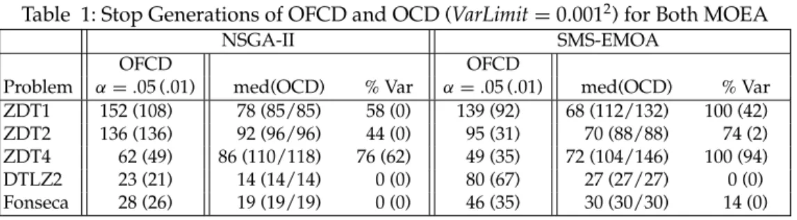
Table 1: Stop Generations of OFCD and OCD (VarLimit=0.0012_{) for Both MOEA}

NSGA-II SMS-EMOA

OFCD OFCD

Problem α=.05 (.01) med(OCD) % Var α=.05 (.01) med(OCD) % Var ZDT1 152 (108) 78 (85/85) 58 (0) 139 (92) 68 (112/132) 100 (42)

ZDT2 136 (136) 92 (96/96) 44 (0) 95 (31) 70 (88/88) 74 (2)

ZDT4 62 (49) 86 (110/118) 76 (62) 49 (35) 72 (104/146) 100 (94)

DTLZ2 23 (21) 14 (14/14) 0 (0) 80 (67) 27 (27/27) 0 (0)

Fonseca 28 (26) 19 (19/19) 0 (0) 46 (35) 30 (30/30) 14 (0)

and α=.01 (OFCD) in order to investigate the dependence on the parametrisation. For measuring the performance of the algorithms, the following PI have been used: hypervolume (HV; Zitzler and Thiele, 1998), additive ε(Eps; Zitzler et al., 2003), and R2 (Hansen and Jaszkiewicz, 1998). OCD terminates if and only if at least one of the tests (χ2variance orttest on ˆβ) indicates convergence with respect to all three metrics simultaneously.

In order to enable the computation of the quality loss of the stop generation com-pared toMaxGenin the online approach, the PIs were additionally calculated atMaxGen

and the OCD stop generation for all runs using a discrete approximation of the true Pareto front as the reference front. These reference fronts also used within OFCD have been calculated via equidistant sampling of the known Pareto fronts.

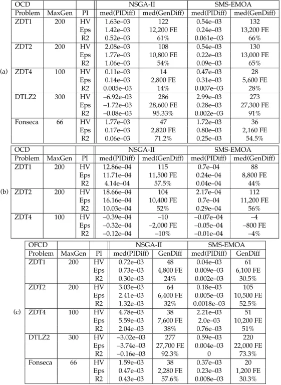
Results/visualisation. Table 1 compares the stop generations obtained for different parameterisations of OFCD and OCD. For OCD, the percentage of runs terminated by variance criterion is given in addition; for OFCD, different values ofαare tested, brackets reveal results for (VarLimit=0.00012_{/Only Regression Criterion) within the} columns of OCD. Table 2 displays the saved function evaluations that have been possible applying the corresponding convergence detection methods and the resulting loss in quality, which has to be accepted. The table consists of three subtables, where the two upper ones provide the results from OCD featuring different VarLimitvalues (0.0012 upper table, 0.00012_{middle one), the lower one presents the results for OFCD featuring} α=.05. The loss of quality is calculated by the difference of the normalised performance indicators (Wagner et al., 2009) at the computed stop generation and the ones obtained performing all function evaluations (MaxGen) suggested in the literature (Deb et al., 2003). In addition, the number of saved function evaluations and their percentage of the recommend ones are reported; forVarLimit=0.00012_{only the problems where the} variance criterion terminates in some of the runs are given.

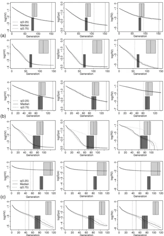
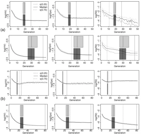
Figures 1 and 2 provide a visual analysis of the different stopping criteria. The results for the ZDT test functions (ZDT1 in the upper group, ZDT2 in the middle group, and ZDT4 in the lower group) are provided in Figure 1. Figure 2 depicts the corresponding plots for the Fonseca test function (upper group) and DTLZ2 (lower group).

Observations. OCD with default settings manages to save at least 20% of the function evaluations recommended in literature (Deb et al., 2003)—in most cases a lot more (Table 2). Simultaneously, a high accuracy of the optimisation result is ensured by keeping the PI loss with respect to the maximum generation number (MaxGen) in the range of the specified variance limit (VarLimit) of theχ2_{variance test. With decreasing}

Table 2: (a) OCD,VarLimit=0.0012_{; (b) OCD,VarLimit=0.0001}2_{; (c) OFCD,α=.05;} Summary of PI and Generation Differences at the Stop Generation andMaxGen, where PIDiff=PIj,Stop−PIj,MaxGenand GenDiff=MaxGen−Stop, (j = {H V , Eps, R2}).

(a)

OCD NSGA-II SMS-EMOA

Problem MaxGen PI med(PIDiff) med(GenDiff) med(PIDiff) med(GenDiff)

ZDT1 200 HV 1.63e–03 122 0.54e–03 132

Eps 1.42e–03 12,200 FE 0.24e–03 13,200 FE

R2 0.52e–03 61% 0.061e–03 66%

ZDT2 200 HV 2.08e–03 108 0.54e–03 130

Eps 1.77e–03 10,800 FE 0.22e–03 13,000 FE

R2 1.06e–03 54% 0.09e–03 65%

ZDT4 100 HV 0.11e–03 14 0.47e–03 28

Eps 0.14e–03 2,800 FE 0.31e–03 5,600 FE

R2 0.005e–03 14% 0.007e–03 28%

DTLZ2 300 HV –6.92e–03 286 2.99e–03 273

Eps –1.72e–03 28,600 FE 0.28e–03 27,300 FE

R2 –0.08e–03 95.33% 0.002e–03 91%

Fonseca 66 HV 1.77e–03 47 1.72e–03 36

Eps 0.17e–03 2,820 FE 0.80e–03 2,160 FE

R2 0.06e–03 71.2% 0.25e–03 54.5%

(b)

OCD NSGA-II SMS-EMOA

Problem MaxGen PI med(PIDiff) med(GenDiff) med(PIDiff) med(GenDiff)

ZDT1 200 HV 12.86e–04 115 0.7e–04 88

Eps 11.71e–04 11,500 FE 0.24e–04 8,800 FE

R2 4.14e–04 57.5% 0.04e–04 44%

ZDT2 200 HV 18.66e–04 104 2.17e–04 112

Eps 16.16e–04 10,400 FE 0.7e–04 11,200 FE

R2 10.03e–04 52% 0.29e–04 56%

ZDT4 100 HV –0.39e–04 –10 –0.07e–04 –4

Eps –0.32e–04 –2,000 FE –0.05e–04 –800 FE

R2 –0.12e–04 –10% –0.01e–04 –4%

(c)

OFCD NSGA-II SMS-EMOA

Problem MaxGen PI med(PIDiff) GenDiff med(PIDiff) GenDiff

ZDT1 200 HV 0.72e–03 48 0.04e–03 61

Eps 0.73e–03 4,800 FE 0.009e–03 6,100 FE

R2 0.30e–03 24% 0.002e–03 30.5%

ZDT2 200 HV 3.03e–03 64 0.18e–03 105

Eps 2.41e–03 6,400 FE 0.005e–03 10,500 FE

R2 1.32e–03 32% 0.0018e–03 52.5%

ZDT4 100 HV 4.78e–03 38 2.21e–03 51

Eps 5.59e–03 7,600 FE 2.0e–03 10,200 FE

R2 2.04e–03 38% 0.76e–03 51%

DTLZ2 300 HV –3.02e–03 277 0.59e–03 220

Eps –3.74e–03 27,700 FE 0.004e–03 22,000 FE

R2 –0.16e–03 92.3% 0 73.3%

Fonseca 66 HV 1.59e–03 38 0.37e–03 20

Eps 0.47e–03 2,280 FE 0.23e–03 1,200 FE

Figure 2: Median, lower, and upper quartile of indicator values of all 50 runs on (a) Fon-seca and (b) DTLZ2 at each generation (NSGA-II: top, SMS-EMOA: bottom). Overall (solid vertical line) and PI-specific offline (OFCD, α=.05) stop generation (dashed vertical line) are marked. Vertical boxplots (light gray:VarLimit=0.00012_{, dark gray:}

VarLimit=0.0012_{) show the distribution of online (OCD) stop generations.}

criterion (Table 1, Figures 1 and 2). This leads to a smaller PI loss, approximately in the interval of [10-04_,10-03_{]. For ZDT2, the recommendedMaxGenare closest toOCDStop,} whereas the opposite is true for DTLZ2 where more than 90% of the generations are spent without improvement.

The OCD boxplots in Figures 1 and 2 often show increasing variability in the distribution of OCD stop generations with decreasing VarLimit. Also, a shift of the distribution toward higher generation numbers can be observed, except for the test problems that are nearly exclusively terminated by the regression criterion.

The stop generations of OFCD withα=.05 (default) match with an intuitive MOEA termination received from visually analysing Figures 1 and 2. Except for ZDT4, OFCD-Stop is higher than the median OCD stop generation. Surprisingly, the SMS-EMOA is stopped on ZDT4 although it progresses in all three PI. Note that at the same time, the variance between runs increases. However, a case of divergence (NSGA-II on DTLZ2) is detected—the suggested stop generation generally fits well with human intuition.

The median PI differences are approximately of size 10-3_{(Table 1). There is a wide} range of saved FE with regard to the test problems (24% up to even more than 90%), and generally these values are slightly smaller than the ones for OCD. In case the α level of the KS tests is decreased to a level ofα=.01, the OFCD criterion becomes less sensitive and results in lower stop generations (Table 1).

The KS test is performed separately for each PI leading to a PI-specific offline stop generation, which is marked in Figures 1 and 2 by a dashed vertical line. The termination of SMS-EMOA is nearly always indicated by the hypervolume (HV) indicator, but for the NSGA-II, the last satisfied criterion can be the HV orεindicator (ZDT4, DTLZ2). R2 indicator curves show the most fluctuating shape over time, especially for the Fonseca problem.

Discussion. OCD and OFCD show obvious differences. It can be generally concluded that OFCD detects convergence later than OCD. This is no surprise as OFCD always takes a set of runs into account and should detect the point when continuing any of the runs is unreasonable. Furthermore, the observation is related to the fact that the dependencies of PIs of successive generations are not taken into consideration in order to ensure the applicability of the KS test. In contrast, OCD always acts on the level of

oneconcrete run. A spread of OCD stop generations is thereby intended and reflects the differences between runs. The experiment shows that most investigated cases comply with this expectation, the only exception being ZDT4. While for OCD, the desired level of approximation quality can be expressed byVarLimitand stagnation is assessed in the regression analysis, OFCD detects stationarity in the distribution of indicator values over all performed runs. Thereby, both situations, which are separately analyzed by OCD, can be detected by the KS test of OFCD. On the one hand, the indicator values indeed stagnate, but on the other hand, the variation of indicator values over different runs gives a limit for improvements that can be detected. Figures 1 and 2 document this fact. Whenever OFCD detects convergence in cases of further improvements, the variation of indicator values over the runs, which is depicted by the interquartile ranges, exceeds the current median value. This can be observed for the SMS-EMOA on ZDT4 or the R2 indicator on Fonseca. This fact is particularly interesting with respect to the application of OFCD for algorithm comparison. Whenever statistical tests are used to evaluate the significance of the results, the variation of indicator values within each algorithm gives a limit for detectable differences. A higher accuracy in the detection of the optimum would not provide a benefit, but spends unnecessary computational resources.

the run is terminated if all tests detect convergence. In OCD, the indicators are com-bined before the test is conducted. Thus, it realises a kind of majority decision. This is advantageous in the given tests because the method stops when the ε and hyper-volume indicator stagnate, despite the R2 indicator continuing to improve. As Table 2 shows, no unbounded improvement of the R2 indicator has been given away. This behavior is related to the selection scheme applied in the corresponding MOEA. While the SMS-EMOA is hypervolume-based, the NSGA-II utilises the nondominated sorting procedure. Thus, it especially focuses on the hypervolume andεindicator. No specific aggregation-based algorithm has been considered. Surprisingly, the indicators actually applied in the MOEA are those for which convergence is detected last when OFCD is used. This may be due to a lower variation in these indicators as described above.

The parameter variation documents that both methods can be intuitively adjusted by their control parameters. The fact that OFCD becomes less sensitive with decreasingα level is due to the termination in cases when the null hypothesis of equal distributions can no longer be rejected. The VarLimitof OCD shows a close relation to the results that can be expected. In cases where the regression criterion has not stopped the run before, the maximum quality difference to the result after the recommended number of generations can be limited to the magnitude of VarLimit(Table 2[a,b]). The larger confidence regions in the boxplots can be explained by two reasons. A lowerVarLimit

entails a higher influence of the stochastic effects. Furthermore, more and more runs are terminated due to the regression criterion ifVarLimitdecreases.

4

Conclusions

In this paper, two recently proposed methods for convergence detection are analysed and systematically compared. The application of these methods to different MOEA and a wide range of test problems documents their successful application as well as their ro-bustness with respect to changing characteristics of performance-indicator trajectories. The systematic differences between the methods are revealed and described. According to their different application levels (OFCD: many runs, offline, OCD: one run, online), the two methods show different characteristics. The method for offline convergence detection efficiently detects the generation in which all indicators stagnate or the im-provement falls below the level of variation between the runs. In contrast, the online method has to respond to the course of one concrete run. The experimental analysis shows that stagnation can be detected or the desired accuracy can be obtained by the in-terplay of a criterion based on variance and one that indicates if the majority of indicator values has converged (regression criterion). In summary, OFCD and OCD each are well suited to their corresponding application area and reliably stop MOEA runs according to a maximum loss, which is predefined (OCD) or detected from the data (OFCD).

References

Beume, N. (2009). S-metric calculation by considering dominated hypervolume as Klee’s measure problem.Evolutionary Computation, 17(4):477–492.

Beume, N., Naujoks, B., and Emmerich, M. (2007). SMS-EMOA: Multiobjective selection based on dominated hypervolume.European Journal of Operational Research, 181(3):1653–1669.

Deb, K., and Jain, S. (2002). Running performance metrics for evolutionary multi-objective optimization. In Proceedings of the 4th Asia-Pacific Conference on Simulated Evolution and Learning (SEAL), pp. 13–20.

Deb, K., Lele, S., and Datta, R. (2007). A hybrid evolutionary multi-objective and SQP based procedure for constrained optimization. In Proceedings of the International Symposium on Intelligence Computation and Applications,L. Kang et al. (Eds.), pp. 36–45. LNCS 4683, Berlin: Springer.

Deb, K., Mohan, M., and Mishra, S. (2003). A fast multi-objective evolutionary algorithm for finding well-spread Pareto-optimal solutions. KanGAL report 2003002, Indian Institute of Technology, Kanpur, India.

Deb, K., Pratap, A., and Agarwal, S. (2002a). A fast and elitist multi-objective genetic algorithm: NSGA-II.IEEE Transactions on Evolutionary Computation, 6(2):182–197.

Deb, K., Thiele, L., Laumanns, M., and Zitzler, E. (2002b). Scalable multi-objective optimization test problems. InCongress on Evolutionary Computation (CEC), Vol. 1, pp. 825–830. Piscataway, NJ: IEEE Press.

Dudoit, S., and van der Laan, M. (2008). Multiple testing procedures with applications to genomics. Berlin: Springer.

Fonseca, C. M., and Fleming, P. J. (1995). Multiobjective genetic algorithms made easy: Selection, sharing, and mating restriction. InProceedings of the 1st International Conference on Genetic Algorithms in Engineering Systems: Innovations and Applications, pp. 42–52.

Guerrero, J. L., Garcia, J., Marti, L., Molina, J. M., and Berlanga, A. (2009). A stopping criterion based on Kalman estimation techniques with several progress indicators. InGECCO ’09: Proceedings of the 11th Annual Conference on Genetic and Evolutionary Computation, pp. 587– 594.

Hanne, T. (1999). On the convergence of multiobjective evolutionary algorithms.European Journal of Operational Research, 117(3):553–564.

Hansen, M. P., and Jaszkiewicz, A. (1998). Evaluating the quality of approximations to the non-dominated set. Technical Report IMM-REP-1998-7, Institute of Mathematical Modeling, Technical University of Denmark.

Hansen, N. (2008). The CMA evolution strategy: A tutorial. Retrieved January 21, 2009, from http://www.bionik.tu-berlin.de/user/niko/cmatutorial.pdf.

Hansen, N., and Ostermeier, A. (2001). Completely derandomized self-adaptation in evolution strategies.Evolutionary Computation, 9(2):159–195.

Hernandez, G., Wilder, K., Nino, F., and Garcia, J. (2005). Towards a self-stopping evolutionary algorithm using coupling from the past. InGECCO ’05: Proceedings of the 2005 Conference on Genetic and Evolutionary Computation, pp. 615–620.

Hoos, H., and St ¨utzle, T. (2004). Stochastic local search—Foundations and applications. San Mateo, CA: Morgan Kaufmann.

Ihaka, R., and Gentleman, R. (1996). R: A language for data analysis and graphics. Journal of Computational and Graphical Statistics, 5:299–314.

Jensen, M. T. (2003). Reducing the run-time complexity of multiobjective EAs: The NSGA-II and other algorithms.IEEE Transaction on Evolutionary Computation, 7(5):503–515.

Kung, H. T., Luccio, R., and Preparata, F. P. (1975). On finding the maxima of a set of vectors. Journal of the Association for Computing Machinery, 22(4):469–476.

Laumanns, M. (2003).Analysis and applications of evolutionary multiobjective optimization algorithms. PhD thesis, Computer Engineering and Networks Laboratory, ETH Zurich, Switzerland.

Laumanns, M., Thiele, L., Deb, K., and Zitzler, E. (2002). Combining convergence and diversity in evolutionary multi-objective optimization. Evolutionary Computation, 10(3):263–282.

Mart´ı, L., Garc´ıa, J., Berlanga, A., and Molina, J. M. (2007). A cumulative evidential stopping criterion for multiobjective optimization evolutionary algorithms (extended version). In D. Thierens, K. Deb, M. Pelikan, H.-G. Beyer, B. Doerr, R. Poli, and M. Bittari (Eds.),GECCO ’07: Proceedings of the 2007 GECCO Conference Companion on Genetic and Evolutionary Computation, pp. 2835–2842.

Mart´ı, L., Garc´ıa, J., Berlanga, A., and Molina, J. M. (2009). An approach to stopping criteria for multi–objective optimization evolutionary algorithms: The MGBM criterion. In2009 IEEE Conference on Evolutionary Computation (CEC 2009), pp. 1263–1270.

Naujoks, B., and Trautmann, H. (2009). Online convergence detection for multiobjective aero-dynamic applications. In A. Tyrrell (Ed.),2009 IEEE Congress on Evolutionary Computation, pp. 332–339.

Rudenko, O., and Schoenauer, M. (2004). A steady performance stopping criterion for Pareto-based evolutionary algorithms. InProceedings of the 6th International Multi-Objective Program-ming and Goal ProgramProgram-ming Conference, 2004.

Rudolph, G. (2001). Self-adaptive mutations may lead to premature convergence. IEEE Transac-tions on Evolutionary Computation, 5(4):410–414.

Rudolph, G., and Agapie, A. (2000). Convergence properties of some multi-objective evolutionary algorithms. InProceedings of the IEEE Congress on Evolutionary Computation (CEC), pp. 1010– 1016.

Safe, M., Carballido, J. A., Ponzoni, I., and Brignole, N. B. (2004). On stopping criteria for genetic algorithms. In A. L. C. Bazzan and S. Labidi (Eds.),Proceedings of Advances in Artificial Intelligence—SBIA 2004, 17th Brazilian Symposium on Artificial Intelligence, Vol. 3171 ofLecture Notes in Computer Science, pp. 405–413. Berlin: Springer.

Sastry, K. (2007). Single and multiobjective genetic algorithm toolbox for Matlab in C++. Technical Report 2007017, Illinois Genetic Algorithms Laboratory, University of Illinois at Urbana-Champaign.

Schwefel, H.-P. (1995). Evolution and optimum seeking. New York: Wiley.

Sheskin, D. J. (2000). Handbook of parametric and nonparametric statistical procedures. 2nd ed. Boca Raton: Chapman & Hall.

Trautmann, H., Ligges, U., Mehnen, J., and Preuss, M. (2008). A convergence criterion for multi-objective evolutionary algorithms based on systematic statistical testing. In G. Rudolph et al. (Eds.),Parallel problem solving from nature (PPSN), pp. 825–836. Berlin: Springer.

Wagner, T., Beume, N., and Naujoks, B. (2007). Pareto-, aggregation-, and indicator-based methods in many-objective optimization. In S. Obayashi et al. (Eds.), Evolutionary multi-criterion optimization (EMO)(pp. 742–756). Berlin: Springer.

Wanner, E., Guimaraes, F., Takahashi, R., and Fleming, P. (2006). A quadratic approximation-based local search procedure for multiobjective genetic algorithms. In G. G. Yen, S. M. Lucas, G. Fogel, G. Kendall, R. Salomon, B.-T. Zhang, C. A. C. Coello, and T. P. Runarsson (Eds.),Proceedings of the 2006 IEEE Congress on Evolutionary Computation, pp. 938–945.

Zielinski, K., and Laur, R. (2007). Stopping criteria for a constrained single-objective particle swarm optimization algorithm.Informatica, 31(1):51–59.

Zitzler, E., Deb, K., and Thiele, L. (2000). Comparison of multiobjective evolutionary algorithms: Empirical results.Evolutionary Computation, 8(2):173–195.

Zitzler, E., and Thiele, L. (1998). Multiobjective optimization using evolutionary algorithms—A comparative case study.Lecture Notes in Computer Science, 1498:292–301.

Zitzler, E., Thiele, L., and Bader, J. (2008). SPAM: Set preference algorithm for multiobjective optimization. In G. Rudolph et al. (Eds.),Parallel problem solving from nature (PPSN), pp. 847– 858. Berlin: Springer.