University of Pennsylvania
ScholarlyCommons
Publicly Accessible Penn Dissertations
2019
Testing Infection Graphs
Justin Turner Khim
University of Pennsylvania, [email protected]
Follow this and additional works at:
https://repository.upenn.edu/edissertations
Part of the
Statistics and Probability Commons
This paper is posted at ScholarlyCommons.https://repository.upenn.edu/edissertations/3358 For more information, please [email protected].
Recommended Citation
Khim, Justin Turner, "Testing Infection Graphs" (2019).Publicly Accessible Penn Dissertations. 3358.
Testing Infection Graphs
Abstract
We study the following problem: given two graphs G_0 and G_1 defined on a common set of n vertices and a single observation of the statuses of these vertices, i.e. either infected, uninfected, or censored, did the
infection spread on G_0 or G_1? Modern instances of such ``infections'' include diseases such as HIV, behaviors such as smoking, or information such as online news articles. For particular stochastic spreading mechanisms, we give algorithms for this testing problem based on hypothesis discretization and permutation-invariance. Additionally, these methods also lead to confidence sets for parameters that also govern the spread of infection and for the graphs on which the infection spread.
Degree Type
Dissertation
Degree Name
Doctor of Philosophy (PhD)
Graduate Group
Statistics
First Advisor
Zongming Ma
Keywords
automorphisms, discretization, hypothesis testing, social and information networks
Subject Categories
TESTING INFECTION GRAPHS
Justin Turner Khim
A DISSERTATION in
Statistics
For the Graduate Group in Managerial Science and Applied Economics Presented to the Faculties of the University of Pennsylvania
in
Partial Fulfillment of the Requirements for the Degree of Doctor of Philosophy
2019
Supervisor of Dissertation
Zongming Ma
Associate Professor of Statistics
Graduate Group Chairperson
Catherine Schrand
Celia Z. Moh Professor, Professor of Accounting
Dissertation Committee:
Dylan Small
Class of 1965 Wharton Professor of Statistics
Alexander Rakhlin
Associate Professor of Brain & Cognitive Sciences Massachusetts Institute of Technology
Po-Ling Loh
TESTING INFECTION GRAPHS c
○ COPYRIGHT 2019
Justin Turner Khim
This work is licensed under the Creative Commons Attribution NonCommercial-ShareAlike 3.0 License
To view a copy of this license, visit
Acknowledgments:
I would like to thank my family, friends, and teachers for being more or less supportive in getting me to this point.
ABSTRACT
TESTING INFECTION GRAPHS
Justin Khim
Zongming Ma
Contents
Acknowledgments iii
Abstract iv
List of Tables viii
List of Figures ix
1 Introduction 1
I Preliminaries 3
2 Setup 4
2.1 Basic Graph Terminology . . . 4
2.2 A Visual Example . . . 4
2.3 Infection Notation . . . 5
2.4 Models . . . 6
2.4.1 Stochastic Spreading Model . . . 6
2.4.2 Ising Model . . . 7
2.4.3 Censoring . . . 7
2.5 Parameters and Tests . . . 8
2.6 Test Statistics and Thresholds. . . 9
3 Maximum Likelihood and Monotonicity 10 3.1 Maximum Likelihood . . . 10
3.2 Monotonicity . . . 11
3.2.1 Monotonicity in the Ising Model . . . 13
3.3 Discussion . . . 13
3.4 Proofs . . . 13
II Discretization 18 4 Theory 19 4.1 Main Result . . . 19
4.1.2 Hypothesis Testing Algorithm . . . 21
4.1.3 Confidence Set Algorithm . . . 21
4.1.4 Computation . . . 22
4.2 Extensions. . . 23
4.2.1 Likelihood-Based Tests. . . 23
4.2.2 Multidimensional Weights . . . 24
4.2.3 Graph Confidence Sets . . . 28
4.3 An Example . . . 28
4.4 Discussion . . . 30
5 Technical Details 31 5.1 Proofs . . . 31
5.1.1 Discretization Proof . . . 31
5.1.2 Algorithm Proofs . . . 34
5.2 Additional Proofs . . . 35
5.3 Extensions Proofs. . . 36
5.3.1 Threshold Function Test . . . 36
5.3.2 Two Statistic Test . . . 39
5.3.3 Multidimensional Weights . . . 40
5.3.4 Confidence Sets . . . 49
5.4 Ising Model . . . 49
5.5 Auxiliary Lemmas . . . 52
6 Numerical Details 55 6.1 Confidence Set for 𝛽 . . . 55
6.2 Toward a Confidence Set for𝒢 . . . 56
III Permutation 59 7 Theory 60 7.1 Permutation-Invariant Statistics. . . 60
7.1.1 Permutations and Group Actions . . . 60
7.1.2 Invariant Statistics . . . 61
7.2 Main Results . . . 61
7.3 Examples and Risk Bounds . . . 63
7.3.1 The Star Graph as𝒢0 . . . 64
7.3.2 The Star Graph as𝒢1 . . . 65
7.4 A Closer Look at Test Statistics. . . 66
7.4.1 Revisiting Likelihood: Likelihood Ratio and Edges-Within . . . 66
7.4.2 Hunt-Stein Theory for Graph Testing . . . 68
7.5 Discussion . . . 69
8 Technical Details 70 8.1 Further Theoretical Results . . . 70
8.1.2 Composite Null Hypotheses . . . 70
8.1.3 Composite Alternative Hypotheses . . . 71
8.1.4 Conditioning on Censored Vertices . . . 72
8.1.5 Computational Considerations . . . 73
8.1.6 Multiple Infection Spreads . . . 73
8.1.7 Relaxing the Choice of Alternative Graph . . . 74
8.1.8 Random Graphs . . . 75
8.2 Proofs . . . 77
8.2.1 Proofs of Main Results . . . 77
8.2.2 Proofs of Invariances . . . 80
8.2.3 Hunt-Stein . . . 82
8.2.4 Likelihood Ratio . . . 83
8.2.5 Risk Bounds when 𝒢0 is the Star . . . 85
8.2.6 Risk Bounds when 𝒢1 is the Star . . . 87
8.3 Proofs of Corollaries . . . 89
8.3.1 Proof of Corollary 7.3.1 . . . 89
8.3.2 Proof of Corollary 7.3.2 . . . 89
8.3.3 Proof of Corollary 7.3.3 . . . 90
8.3.4 Proof of Corollary 8.1.2 . . . 90
8.4 Proofs of Supporting Lemmas . . . 91
8.4.1 Proof of Lemma 8.2.5 . . . 91
8.4.2 Proof of Lemma 8.2.6 . . . 91
8.4.3 Proof of Lemma 8.3.1 . . . 92
8.5 Auxiliary Lemmas . . . 93
9 Numerical Details 94 9.1 HIV Graph Analysis . . . 94
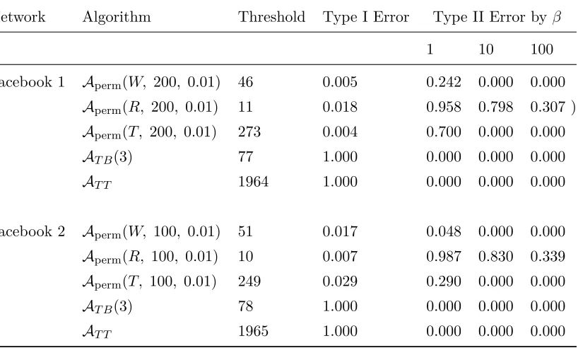
9.2 Simulations . . . 95
9.2.1 Vertex-Transitive Graphs . . . 96
9.2.2 Online Social Network . . . 96
9.2.3 Erdős-Renyi versus Stochastic Block Model Graphs. . . 96
9.2.4 Correlated Erdős-Renyi Random Graphs. . . 99
List of Tables
9.1 Toroidal Grid Simulation Results . . . 97
List of Figures
2.1 The HIV Infection . . . 5
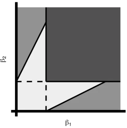
4.1 Discretization Regions for 𝑑= 2 . . . 25
6.1 The HIV Maxcut Partition . . . 55
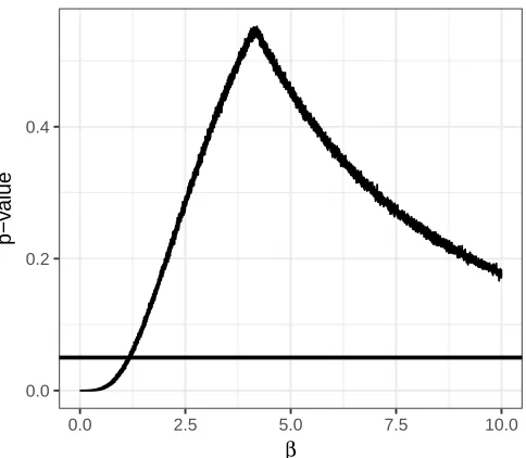
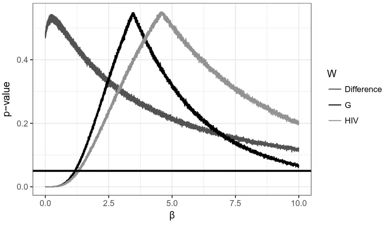
6.2 𝑝-values for the HIV Graph . . . 56
6.3 The Graph 𝒢25 . . . 57
6.4 𝑝-values for𝛽 on 𝒢25 . . . 57
6.5 The Graph 𝒢100 . . . 58
6.6 𝑝-values for𝛽 on 𝒢100 . . . 58
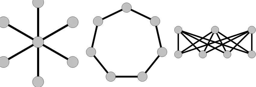
7.1 A 6-Star, a 7-Cycle, and the Complete Bipartite Graph 𝐾3,4 . . . 63
9.1 Simulated Distributions of𝑊 on the HIV graph. . . 94
9.2 The Facebook 1 and Facebook 2 graphs . . . 98
9.3 Erdős-Renyi versus Stochastic Block Model Graph Type I Errors . . . 98
9.4 Erdős-Renyi versus Stochastic Block Model Graph Type II Errors via Permu-tation . . . 99
9.5 Erdős-Renyi versus Stochastic Block Model Graph Type II Errors via Simulation100 9.6 Correlated Erdős-Renyi Graph Type I Errors via Permutation. . . 101
9.7 Correlated Erdős-Renyi Graph Type II Errors via Permutation . . . 101
1.
Introduction
Information, diseases, and the adoption of certain behaviors may spread according to a network of relationships connecting susceptible individuals (Anderson and May, 1992;
Christakis and Fowler, 2007;Jackson,2008;Morris,1993; Newman,2002). Natural questions to address include predicting the pathway or scope of a disease; inferring the source; and identifying nodes or edges at which to intervene in order to slow the spread of the epidemic. The answers to these questions may vary depending on the stochastic mechanism governing the spread of disease between individuals.
Algorithms for addressing such questions often assume knowledge of the underlying graph structure (Borgs et al.,2012; Brautbar and Kearns, 2010; Bubeck et al., 2017). For instance, in the influence maximization problem, the goal is to identify an optimal set of nodes to initially infect in order to propagate a certain behavior as widely as possible (Domingos and Richardson, 2001; Kempe et al., 2003). Due to submodularity of the influence function, one may obtain a constant factor approximation to the influence-maximizing subset using a simple greedy algorithm. However, both the connectivity of the network and edge transmission parameters must be known in order to successfully execute the algorithm (Chen et al.,2010). Similarly, algorithms for network immunization, which aim to eliminate an epidemic by performing targeted interventions, assume knowledge of the graph (Albert et al.,2000;Cohen et al.,2003;Pastor-Satorras and Vespignani,2002). In real-world applications, however, prior knowledge of the edge structure of the underlying network or parameters of the infection spreading mechanism may be unavailable.
Accordingly, the focus of our paper is the inference problem of identifying the underlying network based on observed infection data. One approach involves employing tools from graphical model estimation, since the graphical model corresponding to joint vectors of infection times coincides with the unknown network (Netrapalli and Sanghavi,2012; Gomez-Rodriguez et al., 2016). However, these methods critically leverage the availability of time-stamped data and observations of multiple i.i.d. infection processes spreading over the same graph. Another line of work concerns reconstructing an infection graph based on the order in which nodes are infected over multiple infection processes, and provides bounds on the number of distinct observations required to recover the edge structure of the graph. These methods are attractive in that they do not assume a particular stochastic spreading model, and are even guaranteed to reconstruct the true network when the observations are chosen adversarially (Angluin et al.,2015; Huang et al.,2017). On the other hand, data from multiple infections are still assumed to be available.
spread according to the same mechanisms, and the network may have changed over time. Instead of employing the aforementioned graph estimation procedures based on observation vectors, we cast the problem in the form of a hypothesis test: Given two candidate graphs, our goal is to identify the graph on which the infection has propagated. This type of problem was previously studied byMilling et al.(2015), who proposed inference procedures for testing an empty graph versus graphs satisfying “speed and spread” conditions, and for testing two graphs against each other, critically using an “independent neighborhoods” assumption. A graph testing problem of a somewhat similar flavor may also be found in Bubeck et al.
(2016), but their goal is to identify the model of network formation for a random graph, rather than determine the network underlying an epidemic outbreak.
In this dissertation, we primarily examine two approaches: discretization and permutation. Discretization of the null hypothesis space can be thought of as a computational solution to a particular non-monotonicity for composite hypotheses. Perhaps more elegantly, our permutation approach leverages specific symmetries, vastly reducing computation and leading to permutation tests. We study this approach in more detail.
Permutation testing is notion which dates back to Fisher (1935). Permutation tests are classically applied when random variables are exchangeable under the null hypothesis. The test statistic is then computed with respect to random permutations of the observation vector, and the observed statistic is compared to quantiles of the simulated distribution (Good,2013). We adapt this technique in a novel manner to the graph testing problem. The procedure is the same as in classical permutation testing, where we recompute a certain statistic on a set of randomly chosen permutations of the infection “vector” recording the observed statuses of the nodes in the graph. Based on quantiles of the empirical histogram, we calculate a rejection rule for the test.
The key idea is that if the null hypothesis corresponds to an empty or complete graph and edge transmission rates are homogeneous, the components of the infection vector are certainly exchangeable. This is an important setting in its own right, since it allows us to determine whether a network structure describes an infection better than random noise. However, the permutation test succeeds more generally under appropriate assumptions incorporating symmetries of both the null graph and alternative graph.
A scientific motivation for graph hypothesis testing is a case when a practitioner wants to decide whether a disease is spreading according to a fixed hypothesized graph structure versus completely random transmissions, which would correspond to an empty graph. Another plausible scenario is when a scientist wants to test a long-standing hypothesis that a genetic network follows a particular connectivity pattern, versus a proposed alternative involving the addition or removal of certain edges. In a third setting, one might encounter two distinct graphs representing connections between individuals on different social network platforms, and hypothesize that information diffusion is governed by one graph instead of the other.
Part I
2.
Setup
In this chapter, we introduce our stochastic models and our testing problem. First though, we provide some preliminaries on graph theory and a visual example that we shall return to throughout our numerical analyses.
2.1
Basic Graph Terminology
The primary mathematical object of interest for us is a graph. A graph 𝒢 is a pair of sets 𝒢 = (𝒱,ℰ), where the elements of 𝒱 are called vertices and the elements of ℰ are callededges. For simplicity, we consider the vertices 𝒱 ={1, . . . , 𝑛}. Now, an edge 𝑒 is a pair of vertices 𝑒 = (𝑢, 𝑣). If the edges are unordered, then the resulting graph is called an undirected graph. Otherwise, the graph is a directed graph. For our results, we shall primarily deal with undirected graphs, although for our discretization results, the graphs may be directed without changing the results. Note that we use the words “network” and “graph” interchangeably.
Additionally, we are interested in considering edge weights for our graphs. Given a function 𝑤:ℰ →R+, we say that𝑤(𝑒) is theweight of an edge 𝑒. If a graph𝒢 has an edge weight function 𝑤, then we say that𝒢 is a graph with weighted edges. For our permutation results, we shall restrict ourselves to unweighted graphs, which we can think of as 𝑤(𝑒) = 1 for an edge𝑒.
Finally, one last standard definition is the cut of a graph. A cut 𝐶 is a partition of the vertices into two sets 𝐶 = (𝑈, 𝑉). The cut-set consists of the edges with one vertex in𝑈 and one vertex in𝑉. A maximum cut, usually abbreviated maxcut, is a cut that maximizes the weight of the cut.
2.2
A Visual Example
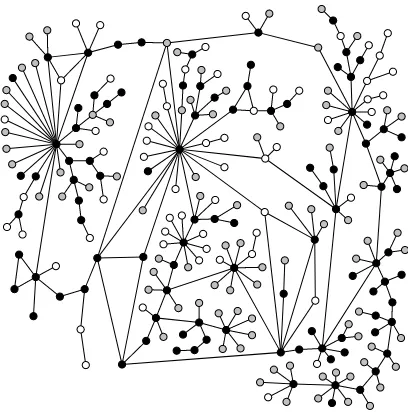
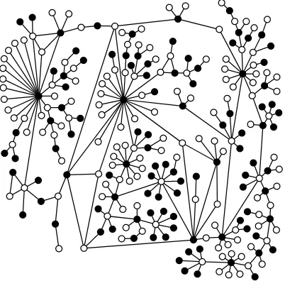
An ongoing example that we consider when applying our analyses is an HIV network. The network is constructed from the population of Colorado Springs from 1982–1989, and the observed infection statuses of individuals, obtained from the CDC and the HIV Counseling and Testing Center, is reported in Potterat et al.(2002). Here, the infection statuses are infected, uninfected, and censored, meaning that the HIV infection status was not observed. For a visualization of the network, see Figure2.1. The network was constructed from contact tracing for sexual and injecting drug partners; beginning in 1985, officials interviewed people testing positive for HIV for information to identify relevant partners.
Figure 2.1The HIV infection graph. Black vertices are infected, white vertices are uninfected, and gray vertices are censored. Edges represent sexual or injecting drug use relationships. Adapted by permission from BMJ Publishing Group, Ltd. [Sexually Transmitted Infections, Potterat et al., 78, i159–i163, 2002]
for explaining the infection. It is quite easy to imagine this in other settings, such as online social networks. In particular, Myers et al. (2012) observed that in such settings, many infections do not occur over the edges of the observed network.
2.3
Infection Notation
Let𝒢0 = (𝒱,ℰ0) and𝒢1 = (𝒱,ℰ1) denote two graphs defined over a common set of vertices
𝒱 ={1, . . . , 𝑛}.We define weight functions𝑤0:ℰ0 →R+ and𝑤1:ℰ1 →R+, where 𝑤𝑖(𝑒) is
the weight of the edge𝑒in𝒢𝑖.
A random vector of infection statuses ℐ :={ℐ𝑣}𝑣∈𝒱 consists of entries
ℐ𝑣 = ⎧ ⎪ ⎪ ⎨
⎪ ⎪ ⎩
1, if𝑣 is infected, 0, if𝑣 is uninfected,
⋆, if𝑣 is censored.
Let ℐ1 denote the set of infected vertices, and let ℐ0 and ℐ⋆ be defined analogously. We
then define the space of possible infection status vectors involving exactly𝑘infected vertices, 𝑐 censored vertices, and𝑛−𝑘−𝑐 uninfected vertices:
I𝑘,𝑐= {︁
2.4
Models
In this section, we introduce our main spreading model. We also define an Ising model, against which we compare our spreading model in a few situations. Finally, we discuss a general methods of censoring that may be applied in either model.
2.4.1 Stochastic Spreading Model
Our main infection model includes the following components: spreading by contagion along edges of the network, and spreading via factors external to the network. The rates of spreading are governed by the nonnegative parameter 𝛽 ∈R+. We assume that an infection spreads on𝒢, beginning at time 0, as follows:
(i) For each vertex 𝑣, generate an independent random variable 𝑇𝑣 ∼Exp(1).
(ii) For each edge (𝑢, 𝑣)∈ ℰ, generate an independent random variable𝑇𝑢𝑣∼Exp(𝛽𝑤(𝑢, 𝑣))
where 𝑤is the weight function.
(iii) For each vertex 𝑣, define the infection time 𝑡𝑣 := min𝑢∈𝑁(𝑣){𝑡𝑢+𝑇𝑢𝑣} ∧𝑇𝑣, where
𝑁(𝑣) is the set of neighbors of𝑣.
In other words, each vertex 𝑣 contracts the disease via random infection according to an exponential random variable with rate 1, and contracts the disease from an infected neighbor 𝑢 at rate 𝛽𝑤(𝑢, 𝑣) relative to random infection; in particular, when 𝒢 is an empty graph, each successively infected node is chosen uniformly at random. The presence of the random variable𝑇𝑣 has the interpretation that some factors involved in spreading the disease may
not be fully accounted for in the hypothesized graphs. We define 𝑡𝑘 to be the time at which
the𝑘th reporting node becomes infected, and we suppose we observe the state of the graph at some time𝑡 such that𝑡𝑘≤𝑡≤𝑡𝑘+1. Note that this differs from other settings, where the
time 𝑡at which the node infection statuses are observed is assumed to be a known constant (Kesten,1993;Milling et al.,2015;Shah and Zaman,2011).
In our analysis, we rely on the notion ofpaths. A path𝑃 = (𝑃1, . . . , 𝑃𝑘) is an ordered set of
vertices, and vertex𝑃𝑖is the𝑖thvertex to be infected. A given infection𝐽 inI𝑘,0 corresponds
to 𝑘! possible paths, which we collect into a setP(𝐽). We also refer to the path random variable as𝒫. Thus, we have the relation
P(ℐ =𝐽) = ∑︁
𝑃∈P(𝐽)
P(𝒫 =𝑃),
which we will use in our derivations. Additionally, we denote𝑃1:𝑡= (𝑃1, . . . , 𝑃𝑡).
To understand the notation we shall use in computing path probabilities, suppose 𝑘vertices have been infected in running the process at time 𝑡, and we want to determine the (𝑘+ 1)th infected vertex. Since all of the𝑇𝑣’s and𝑇𝑢𝑣’s are independent exponential random variables,
the probability that vertex 𝑣 is infected next is
P(𝑣 is infected next|𝒫1:𝑡−1=𝑃1:𝑡−1) =
1 +𝛽𝑊𝑡,𝑣(𝑃1:𝑡−1)
(𝑛−𝑘) +𝛽𝑊𝑡(𝑃1:𝑡−1)
where𝑊𝑡(𝑃1:𝑡−1) is the sum of the weights of edges with one infected vertex at time 𝑡, and
𝑊𝑡,𝑣(𝑃1:𝑡−1) is the sum of the weights𝑤(𝑢, 𝑣) where𝑢 is infected.
We make a few additional remarks on notation. First, when the edges are unweighted, we use 𝑁𝑡 and𝑁𝑡,𝑣 instead of𝑊𝑡and𝑊𝑡,𝑣 to emphasize the the count of neighbors is not weighted.
Finally, if 𝑃 is a path of length 𝑡′ and𝑡 < 𝑡′,𝑁𝑡,in(𝑃) is equivalent to𝑁𝑡,𝑃𝑡(𝑃1:𝑡−1).
Now, note that we consider the case𝛽=∞. Here, uniform spread only occurs when there are no edges between infected and uninfected vertices, i.e. when 𝑊𝑡= 0. One theoretical benefit
is that this allows for the compactness of our parameter space and space of distributions, although this is not necessary for our results.
Finally, we denote an infection ℐ over a graph 𝒢 with parameter 𝛽 byℐ ∼SSM(𝒢, 𝛽). This simplifies the statements of our hypothesis tests.
2.4.2 Ising Model
We now describe an Ising model parametrized by 𝛽 ∈ R+. Define the energy function
ℋ:I𝑘,0 →Rby
ℋ(𝐽) :=− ∑︁
(𝑢,𝑣)∈ℰ
𝑤(𝑢, 𝑣)𝐽𝑢𝐽𝑣 =−𝑊(𝐽),
where 𝑊 is the edges-within statistic that we discuss in further detail in Section 2.6. We define the uncensored Ising model by
P𝑢Ising(ℐ =𝐽) :=
exp(−𝛽ℋ(𝐽))
∑︀ 𝐽′∈
I𝑘,0exp(−𝛽ℋ(𝐽
′)) =
1 𝑍Ising,𝑘(𝛽)
exp(−𝛽ℋ(𝐽)).
Note that this resembles an Ising model with −1 replaced by 0. For simplicity, we denote an infectionℐ generated by the Ising model on graphset𝒢with parameter𝛽 byℐ ∼Ising(𝒢, 𝛽).
Since the Ising model does not have a spreading interpretation, this is not our model of interest. However, in certain regimes, the stochastic spreading model behaves similarly to the Ising model. Finally, at other points, the Ising model provides a stark contrast to our stochastic spreading model.
2.4.3 Censoring
Our model permits vertex statuses to be censored. The two models of censoring we consider are uniform censoring and fixed censoring. We consider the uniform spreading model here as an example, and we further study the fixed censoring variant in Chapter 8, since the precise details are most important for our permutation results.
uncensored vertex𝑣. We then define the measure
𝜇(𝐽;𝛽) = ∑︁
𝐽′∈𝒰(𝐽)
1
(︀𝑛
𝑐
)︀P
𝑢(︀ℐ
=𝐽′)︀
,
whereP𝑢(ℐ=𝐽′) denotes the probability of an uncensored infection from the model described
above. In other words, 𝜇 simply computes the probability of observing a vector 𝐽 after randomly censoring𝑐 nodes. If we define the normalizing constant
𝑍(𝛽) := ∑︁
𝐽∈I𝑘,𝑐
𝜇(𝐽;𝛽) = ∑︁
𝐽∈I𝑘,𝑐 ∑︁
𝐽′∈𝒰(𝐽)
1
(︀𝑛
𝑐
)︀P
𝑢(ℐ =𝐽′
),
which provides the probability of observing any vector with 𝑐 censored nodes, we see that
P(ℐ =𝐽) =
1
𝑍(𝛽)𝜇(𝐽;𝛽)
is the probability of observing infection vector 𝐽, conditioned on 𝑐 nodes having been censored. Note that in the case when𝒢 is the empty graph, the values of 𝜇(𝐽;𝛽) are the same for all values of 𝐽, so P(ℐ) = 1/|I𝑘,𝑐|= 1/(︀𝑘 𝑐𝑛 )︀, i.e. the inverse of the multinomial
coefficient for choosing 𝑘and 𝑐 items from a set of𝑛.
2.5
Parameters and Tests
In this section, we describe our hypothesis testing and confidence set framework. To this end, we start by more fully detailing the notation of our parameters. Let 𝒢0 and 𝒢1 be
graphs with possibly weighted edges. LetB0 and B1 be sets of possible𝛽 values, and these
are subsets of the natural parameter spaces C0 and C1. A graph-parameter pair (𝒢𝑖, 𝛽) parametrizes a probability measureP𝑖,𝛽 by ℳ(𝒢𝑖, 𝛽) =P𝑖,𝛽, andP𝑖,𝛽 can be thought of as
an element of the probability simplex with entries indexed by the infections of I𝑘,𝑐. Note that we sometimes write our parameters as 𝜃= (𝒢, 𝛽), and the resulting parameter space is then Θ.
Now, our hypothesis tests have the following form:
𝐻0 :ℐ ∼SSM(𝒢0, 𝛽0) for 𝛽0 ∈B0, 𝒢0∈G0
𝐻1 :ℐ ∼SSM(𝒢1, 𝛽1) for 𝛽1 ∈B1, 𝒢1∈G1.
In most sections, we only consider a “simple” hypothesis test whereG0 andG1 are singleton sets. Via duality, we can define confidence sets as the set of (𝒢0, 𝛽0) for which the test was
not rejected.
At this point, we make some of these sets more concrete. Our primary hypothesis testing problem has
C0 =C1 =R+= [0,∞].
In general, a reasonable choice of parameter sets might beB0 = [0,∞] and B1 = (0,∞].
overlap, so the minimum power of any valid test is at most 𝛼. Thus, to provably attain non-trivial power, one could take the standard approach of designating an indifference region, so that B1 = [𝑐,∞] for some𝑐 >0.
A critical function 𝜓:I𝑘,𝑐→ {0,1} may be used to indicate the result of a test. We will be interested in bounding the risk, which is the sum of Type I and Type II errors:
𝑅𝑘,𝑐(𝜓;𝛽0, 𝛽1) =P0,𝛽0(𝜓(ℐ) = 1) +P1,𝛽1(𝜓(ℐ) = 0).
2.6
Test Statistics and Thresholds
In general, we would like to use any test statistic𝑆 :I𝑘,𝑐 →R. However, in PartIIIwhen we consider permutations, we shall have to make some restrictions. Without loss of generality, we reject the null hypothesis for large values of𝑆. An important statistic for our analyses is the edge weights within an infection
𝑊(𝐽) := ∑︁
(𝑢,𝑣)∈ℰ
𝑤(𝑢, 𝑣)1{𝐽𝑢=𝐽𝑣 = 1}.
For a fixed value of𝛽, we define the (1−𝛼)-quantile of𝑆(ℐ) to be
𝑡𝛼,𝛽 := sup{𝑡∈supp(𝑆) :P𝛽(𝑆(ℐ)≥𝑡)> 𝛼}
where supp(𝑆) is the support of𝑆, i.e. the set of values that the discrete random variable 𝑆 takes with positive probability. Note that we have the two bounds
P𝛽(𝑆(ℐ)> 𝑡𝛼,𝛽)≤𝛼
P𝛽(𝑆(ℐ)≥𝑡𝛼,𝛽)> 𝛼,
(2.1)
i.e. the strictness of the inequality in the event determines the direction of the inequality in the probability bound.
The tests given in this dissertation are based on simulated null distributions of the test statistic𝑆 in order to approximate 𝑡𝛼,𝛽. To quantify the exact uncertainty introduced by
the simulations, we define the empirical (1−𝛼)-quantile ^𝑡𝛼:I𝑁𝑘,𝑐sims →Rto be
^
𝑡𝛼,𝛽 := sup {︃
𝑡∈supp(𝑆) : 1 𝑁sims
𝑁sims
∑︁
𝑖=1
1{𝑆(𝐼𝑖)≥𝑡} ≥𝛼 }︃
.
Additional Notation
Before proceeding, we comment on a few of our notation conventions. As seen earlier in the case of paths, we use 1 :𝑡to denote a𝑡-tuple. Other examples includeℐ(1:𝑚)= (ℐ(1), . . . ,ℐ(𝑚),
where each ℐ(𝑖) is an infection, and𝑋
1:𝑘+𝑐= (𝑋1, . . . , 𝑋𝑘+𝑐).
For probability measures, we writeP𝑖,𝛽 to denote a probability computed with respect to the
parameters (𝒢𝑖, 𝛽). If our graph is merely 𝒢, we writeP𝛽. In other situations, if we consider
coupled random variables with different parameters, we omit subscripts and writeP. Finally, for a statistic 𝑆, we may write 𝑆𝑖 to denote that the statistic is compute with respect to 𝒢𝑖,
3.
Maximum Likelihood and
Monotonic-ity
In this chapter, we consider two approaches to inference that might be found in an introduc-tory course: maximum likelihood and monotonicity. The first refers to the usual maximum likelihood estimate of parameters, where here the parameters are both the underlying graph
𝒢 and scalar 𝛽. The second is the monotonicity of a𝑝-value or decision threshold as we vary the underlying parameter𝛽. To simplify matters, we shall only consider the case of no censoring, or 𝑐= 0, for this chapter.
3.1
Maximum Likelihood
A first standard approach is to consider maximum lielihood estimation. The good news is that some standard maximum likelihood results are sufficiently general to apply in some sense. However, it is the more standard setting of maximum likelihood estimation in which we are given 𝑚 i.i.d. samples from the same distribution, which would require multiple infections in this case. We let 𝐿(𝒢, 𝛽;𝐽) denote the likelihood. These results follow from Section 3.3 ofLehmann and Romano (2006).
Lemma 3.1.1. Suppose that the distributions SSM(𝒢, 𝛽) are distinct, i.e. the parameters are identifiable. Suppose we receive 𝑚 i.i.d. infections ℐ(1), . . . ,ℐ(𝑚) ∼SSM(𝒢
0, 𝛽0). For any
fixed (𝒢, 𝛽)̸= (𝒢0, 𝛽0) as 𝑚→ ∞, we have
P0,𝛽0
(︁
𝐿(︁𝒢0, 𝛽0;ℐ(1:𝑚)
)︁
> 𝐿(︁𝒢, 𝛽;ℐ(1:𝑚))︁)︁→1.
The proof is identical to that ofLehmann and Romano (2006), and so we omit it. Before stating the proposition, we define the likelihood equation as
𝜕 𝜕𝛽 log𝐿
(︁
𝒢, 𝛽;ℐ(1:𝑚))︁.
Thus a root ^𝛽 of the likelihood equation is just a parameter for which this derivative is 0.
Proposition 3.1.1. Let 𝛽0 be contained in (0,∞). Under the same conditions as the previous
lemma, there is a sequence 𝜃^𝑚 = (︁
^
𝒢𝑚,𝛽^𝑚 )︁
where (i) 𝒢^𝑚 maximizes the likelihood across
graphs, (ii)𝛽^𝑚 are roots of the likelihood equation, and (iii) 𝜃^𝑚 tends to the true parameter value 𝜃0 = (𝒢0, 𝛽0) in probability.
Note that the condition that 𝛽0 be in the open interval from 0 to ∞ is so that we can
𝛽 = 0 makes the graph unidentifiable. A slight modification of the proof would extend the result to the empty graph. Another reason to prefer 𝛽 < ∞ is that it makes it easier to avoid non-identifiability issues. For example, consider the case of a line graph with𝑛= 8 vertices where𝑘= 5 are infected. Then, if 𝛽=∞, the fourth and fifth vertices are always infected, making the underlying graph unidentifiable, even as𝑚 increases. If 𝛽 <∞, then any two vertices can have different infection statuses
Of course, if it has not become obvious yet, the real problem with maximum likelihood estimation is computational. Since our stochastic spreading model requires summing probabilities over paths, in general we would have to sum over 𝑘! paths in order to compute the likelihood for a single infection. Supposing that we wanted to approximate the likelihood, we could try sampling infection paths as follows. Given a single infection𝐽, let 𝑈(𝒢, 𝛽;𝐽) be the random variable defined by
𝑈(𝒢, 𝛽;𝐽) =
{︃
P𝒢,𝛽{𝒫 =𝑃} w.p. 𝑘1! for𝑃 ∈P(𝐽)
0 otherwise.
Then, we have
E[𝑈(𝒢, 𝛽;𝐽)] =
1 𝑘!
∑︁
𝑃∈P(𝐽)
P𝒢,𝛽{𝒫 =𝑈}=
1
𝑘!𝐿(𝒢, 𝛽;𝐽).
If we consider 𝑚uniform samples𝑈1, . . . , 𝑈𝑚, then we can obtain an unbiased estimate of
the likelihood by averaging and scaling, yielding
˜
𝐿𝑚(𝒢, 𝛽;𝐽) :=
𝑘! 𝑚
𝑚 ∑︁
𝑖=1
𝑈𝑖(𝒢, 𝛽;𝐽).
We could define a similar random variable on the log scale if desired. Of course, the major problem is still the𝑘! term, because the variance of ˜𝐿𝑚(𝒢, 𝛽;𝐽) may be very high even for
moderately large 𝑚.
3.2
Monotonicity
Consider the following basic statistical hypothesis test:
𝐻0 : 𝑋 ∼N
(︁
𝜇0, 𝜎2
)︁
𝜇0 ≤0
𝐻1 : 𝑋 ∼N
(︁
𝜇1, 𝜎2
)︁
𝜇1 >0
where 𝜎2 is a known constant. Then, if we consider 𝜇0 = 0, we might reject the null
hypothesis when the 𝑍-statistic
𝑍 = √𝑋
𝜎2
is sufficiently large. In particular, we reject when 𝑍 exceeds the threshold𝑡𝛼, which is given
by
Of course, we determine a𝑝-value for the test numerically by using the fact that𝑍 ∼N (0,1). Now, what if we want to construct a valid test for general𝜇′0 ≤0? If we define a statistic𝑍′ by
𝑍′ = 𝑋−𝜇
′
0 √
𝜎2 =𝑍+𝐶,
where 𝐶 is non-negative. Then, by examining thresholds, we have
𝑡′𝛼= sup{︁𝑧∈supp(𝑍′) :P𝜇 0=𝜇′0
(︀
𝑍′ ≥𝑧)︀
> 𝛼}︁.
Since 𝑍 is a standard normal random variable when𝜇0 = 0 and 𝑍′ is a standard normal
random variable when 𝜇0 =𝜇′0 <0, we observe that the thresholds𝑡𝛼 =𝑡′𝛼. However, in the
latter case, we only require𝑍+𝐶 =𝑍′ > 𝑡𝛼 to reject the null hypothesis, and this is always
satisfied when 𝑍 > 𝑡𝛼. Put another way, we have
𝑡𝛼= sup 𝜇0≤0
sup{𝑧∈supp(𝑍) :P𝜇0(𝑍 ≥𝑧)> 𝛼}= sup{𝑧∈supp(𝑍) :P𝜇0=0(𝑍 ≥𝑧)> 𝛼}
(3.1)
In terms of 𝑝-values, the 𝑝-value obtained for any 𝜇′0<0 is strictly smaller than that of the 𝑝 value for𝜇0= 0. This is a natural monotonicity that simplifies the testing problem from
both a mathematical and computational point of view.
With a clearer idea of what we mean by monotonicity, we consider it in the problem of graph testing. Suppose we have the following testing problem:
𝐻0: ℐ ∼SSM(𝒢0, 𝛽0) 𝛽0 ∈B0
𝐻1: ℐ ∼SSM(𝒢1, 𝛽1) 𝛽1 ∈B1
for some parameter setB0 andB1. Suppose that we use a statistic 𝑆(ℐ), and we reject the null hypothesis when 𝑆(ℐ) is greater than some threshold𝑡𝛼. To control the Type I error at
a level 𝛼, we need to have
𝑡𝛼= sup 𝛽0∈B0
max{𝑠∈supp(𝑆) :P𝒢0,𝛽0(𝑆(ℐ)≥𝑠)> 𝛼}. (3.2)
Unlike equation (3.1), it is far from clear that there is any natural monotonicity that we can use to remove the maximum over the parameter in computing this threshold.
Our first hope might be that the threshold for a simple statistic such as the edges within𝒢0
is monotonically increasing in𝛽0. Indeed, some of our simulation results, this seems to be
the case on the very small number of values of𝛽0 we examine. Unfortunately, this turns out
to not be the case in general. For simplicity, let 𝑡𝛼(𝛽0) be the threshold value with respect
to a single parameter value 𝛽0
Proposition 3.2.1. Consider the hypothesis test
𝐻0 : ℐ ∼SSM(𝒢0, 𝛽0) 𝛽0∈[0,∞]
𝐻1 : ℐ ∼SSM(𝒢1, 𝛽1) 𝛽1∈B1
where 𝒢0 ̸=𝒢1. Fix any level 𝛼, and reject the null hypothesis when 𝑊0 is sufficiently large.
To keep the exposition separate from the proofs, we prove this result in Section 3.4. However, the graph 𝒢0 is very simple to describe. It consists of two connected components, one of which is large but very sparse and the other of which is small but fully connected.
If we were somehow able to rule out such pathological cases with massive disparities in connectivity, perhaps one could prove a monotonicity result. We conjecture that there is a class of graphs for which this is true.
Conjecture 3.2.1. For a fixed𝛼and𝑘 >0, if𝒢0 is a vertex-transitive graph, then the threshold
𝑡𝛼(𝛽0) for the statistic 𝑊0 is monotonically increasing in 𝛽0.
3.2.1 Monotonicity in the Ising Model
While we are mainly interested in our stochastic spreading model, we do note that the desried monotonicity does hold for the Ising model.
Proposition 3.2.2. Consider the hypothesis test
𝐻0: ℐ ∼Ising(𝒢0, 𝛽0) 𝛽0∈B0
𝐻1: ℐ ∼Ising(𝒢1, 𝛽1) 𝛽1∈B1.
Fix any level 𝛼, and reject the null hypothesis when 𝑊0 is sufficiently large. Then, the
threshold 𝑡𝛼 is monotonically increasing as a function of 𝛽.
3.3
Discussion
In this chapter, we discussed maximum likelihood estimation and monotonicity of the thresholds. Both of these techniques have shortcomings that make them insufficient for practical use by themselves, and this is one of the motivations for our discretization and permutation methods. Note that we shall revisit maximum likelihood in the coming chapters, particularly as it relates to discretization and to the permutation statistics.
3.4
Proofs
This section contains proofs of the results of this chapter.
Proof of Proposition 3.1.1. First, we examine the average log-likelihood, which we define as
𝑓(︁𝒢, 𝛽;ℐ(1:𝑚))︁= 1 𝑚
𝑚 ∑︁
𝑖=1
log𝐿(︁𝒢, 𝛽;ℐ(𝑖))︁.
with respect to 𝛽, we have
𝜕 𝜕𝛽𝑓
(︁
𝒢, 𝛽;ℐ(1:𝑚))︁= 1 𝑚 𝑚 ∑︁ 𝑖=1 ⎛ ⎝ ∑︁
𝑃∈P(I𝑘,0) 𝑘 ∏︁
𝑡=1
1 +𝛽𝑊𝑡,𝑣(𝑃)
𝑛+ 1−𝑡+𝛽𝑊𝑡(𝑃) ⎞
⎠
−1
× ∑︁
𝑃∈P(I𝑘,0) 𝑘 ∑︁ 𝑡=1 ⎛ ⎝ ∏︁ 𝑠̸=𝑡
1 +𝛽𝑊𝑠,𝑣(𝑃)
𝑛+ 1−𝑡+𝛽𝑊𝑠(𝑃) ⎞
⎠
× 1
𝑛+ 1−𝑡+𝛽𝑊𝑡(𝑃)
·𝑊𝑡,𝑣(𝑃)(𝑛+ 1−𝑡)−𝑊𝑡(𝑃)
𝑛+ 1−𝑡+𝛽𝑊𝑡(𝑃)
= 1 𝑚 𝑚 ∑︁ 𝑖=1 ∑︁
𝑃∈P(I𝑘,0) 𝑘 ∑︁
𝑡=1
𝑛+ 1−𝑡+𝛽𝑊𝑡(𝑃)
1 +𝛽𝑊𝑡,𝑣(𝑃)
× 1
𝑛+ 1−𝑡+𝛽𝑊𝑡(𝑃)
·𝑊𝑡,𝑣(𝑃)(𝑛+ 1−𝑡)−𝑊𝑡(𝑃)
𝑛+ 1−𝑡+𝛽𝑊𝑡(𝑃)
= 1 𝑚 𝑚 ∑︁ 𝑖=1 ∑︁
𝑃∈P(I𝑘,0) 𝑘 ∑︁
𝑡=1
1 1 +𝛽𝑊𝑡,𝑣(𝑃)
·𝑊𝑡,𝑣(𝑃)(𝑛+ 1−𝑡)−𝑊𝑡(𝑃)
𝑛+ 1−𝑡+𝛽𝑊𝑡(𝑃)
.
Note that this is bounded above by
𝜕 𝜕𝛽𝑓
(︁
𝒢, 𝛽;ℐ(1:𝑚))︁≤ 1
𝑚
𝑚 ∑︁
𝑖=1
∑︁
𝑃∈P(I𝑘,0) 𝑘 ∑︁
𝑡=1
1 1 +𝛽𝑊𝑡,𝑣(𝑃)
· 𝑊𝑡,𝑣(𝑃)(𝑛+ 1−𝑡)
𝑛+ 1−𝑡+𝛽𝑊𝑡(𝑃)
,
so, the derivative has an upper bound of the form
𝜕 𝜕𝛽𝑓
(︁
𝒢, 𝛽;ℐ(1:𝑚))︁≤ 𝑎
𝑏+𝑐𝛽2
for constants𝑎≥0 and𝑏, 𝑐 >0 that can be chosen independently of𝑚. Thus, on an interval [𝛽, 𝛽′] the average log-likelihood is bounded as
𝑓(︁𝒢, 𝛽′′;ℐ(1:𝑚))︁≤𝑓(︁𝒢, 𝛽;ℐ(1:𝑚))︁+
∫︁ 𝛽′
𝛽
𝑎 𝑏+𝑐𝑥2𝑑𝑥
=𝑓(︁𝒢, 𝛽;ℐ(1:𝑚))︁+√𝑎
𝑏𝑐 (︂ arctan (︂ 𝛽′ √︂ 𝑐 𝑏 )︂ −arctan (︂ 𝛽 √︂ 𝑐 𝑏 )︂)︂ .
With this representation, we see that if we pick a sufficiently fine finite discretization B𝐷 of
[0,∞], we can approximate the average likelihood everywhere within an additive factor𝜖. Next, we want to pick𝜖sufficiently small to distinguish the graph 𝒢0 correctly.
Let Δ be defined by
Δ =E𝒢0,𝛽0log𝐿(𝒢0, 𝛽0;ℐ)− sup
𝒢̸=𝒢0,𝛽∈[0,∞]
E𝒢0,𝛽0log𝐿(𝒢, 𝛽;ℐ).
By Jensen’s inequality, we see that
Δ> inf
𝒢̸=𝒢0,𝛽∈[0,∞]
logE𝒢0,𝛽0
𝐿(𝒢0, 𝛽0;ℐ)
with strict inequality since the logarithm is strictly concave. Note that by the law of large numbers,
𝑓(︁𝒢, 𝛽;ℐ(1:𝑚))︁−→a.s. E𝒢0,𝛽0log𝐿(𝒢, 𝛽;ℐ),
so, we have
P {︂
𝑓(︁𝒢0, 𝛽0;ℐ(1:𝑚)
)︁
> 𝑓(︁𝒢, 𝛽;ℐ(1:𝑚))︁+Δ 2
}︂
→1.
At this point, we pick 𝜖= Δ/2, and we define the following event:
𝐸𝑚(𝛿) = {︁
ℐ(1:𝑚)∈I𝑚𝑘,0:𝑓(︁𝒢0, 𝛽0;ℐ(1:𝑚)
)︁
> 𝑓(︁𝒢0, 𝛽0−𝛿;ℐ(1:𝑚)
)︁
𝑓(︁𝒢0, 𝛽0;ℐ(1:𝑚)
)︁
> 𝑓(︁𝒢0, 𝛽0+𝛿;ℐ(1:𝑚)
)︁
𝑓(︁𝒢0, 𝛽0;ℐ(1:𝑚)
)︁
> 𝑓(︁𝒢, 𝛽;ℐ(1:𝑚))︁+𝜖
for all 𝒢 ̸=𝒢0, 𝛽∈B𝐷}.
By Lemma3.1.1and a union bound, we see that for any fixed 𝛿, we have
P0,𝛽0(𝐸𝑚(𝛿))→1.
By a diagonal argument, we can pick a sequence 𝛿𝑚→0 such that
P0,𝛽0(𝐸𝑚(𝛿𝑚))→1
as well.
Now, we can define ^𝜃𝑚 = (︁
^
𝒢,𝛽^𝑚 )︁
. We let ^𝒢𝑚 = 𝒢0 since this maximizes the likelihood
across graphs, and we let ^𝛽𝑚 to be the zero of the derivative of the log-likelihood with
respect to𝛽 under the event 𝐸𝑚(𝛿𝑚) in the interval (𝛽0−𝛿𝑚, 𝛽0+𝛿𝑚). Then we observe
the probability that ^𝛽𝑚 is a root of the likelihood equation is
P0,𝛽0
(︂𝜕𝑓
𝜕𝛽
(︁
^
𝒢𝑚,𝛽^𝑚;ℐ(1:𝑚)
)︁)︂
≥P0,𝛽0(𝐸𝑚(𝛿𝑚))→1.
Finally, we observe that the parameter estimates converge to the true values. Let 𝛿 >0 be an arbitrary constant, and if 𝑚 is sufficiently large, we have
P0,𝛽0
(︁
^
𝒢𝑚=𝒢0, |𝛽^𝑚−𝛽0| ≤𝛿
)︁
≥P0,𝛽0(︁𝒢^𝑚=𝒢0, |𝛽^𝑚−𝛽0| ≤𝛿𝑚 )︁
=P0,𝛽0(𝐸𝑚(𝛿𝑚))→1,
and this completes the proof.
Proof of Proposition 3.2.1. Define a graph𝒢to be the union of two graphs𝒢′and𝒢′′. We let
In the former case, let 𝑋 be the number of infected vertices in𝒢′. Then, we can write
P(︀𝑋=𝑘′)︀=
(︀𝑛′
𝑘′
)︀(︀𝑛′′
𝑘′′ )︀
(︀𝑛
𝑘
)︀ .
Thus, 𝑋 has a Hypergeometric(𝑛′, 𝑛, 𝑘) distribution. By Theorem 1 and Theorem 4 of
Hoeffding(1963), we have the inequality
P(𝑋 ≥(1−𝛼+𝛾+𝑡)𝑘) =P (︂
𝑋≥
(︂𝑛′
𝑛 +𝑡
)︂
𝑘
)︂
≤exp(︁−2𝑡2𝑘)︁. (3.3)
So for any fixed𝑡 >0, this probability can be made arbitrarily small by increasing𝑘.
Let 𝐴 denote the event on the left hand side of equation (3.3), and let 𝑌 =𝑘−𝑋 be the number of infected vertices in𝒢′′. Then under event 𝐴, we see𝑌 ≤(𝛼−𝛾−𝑡)𝑘. Thus, we
can lower bound the threshold𝑡𝛼(0) for the edges within statistic by
(𝛼−𝛾−𝑡)2𝑘2 ≤𝑡𝛼(0)
assuming that the right hand side of equation (3.3) is upper bounded by 𝛼, i.e. when
𝑘≥ 1
2𝑡2 log
1
𝛼. (3.4)
Next, we consider the case where 𝛽 =∞. Then, with probability 1−(𝛼−𝛾), the resulting infection forms a connected subgraph in 𝒢′, and so𝑊(ℐ) =𝑘−1. Thus, we are guaranteed
𝑡𝛼(∞)≤𝑘≤(𝛼−𝛾−𝑡)2𝑘2 ≤𝑡𝛼(0)
when
1
(𝛼−𝛾−𝑡)2 ≤𝑘. (3.5)
For fixed 𝛼, equation (3.4) and equation (3.5) can be satisfied by taking 𝑛 and 𝑘 to be sufficiently large, completing the proof.
Proof of Proposition 3.2.2. For a fixed 𝛽0, let 𝐴 be the set
𝐴={𝐽 :𝑊(𝐽)> 𝑡𝛼(𝛽0)}.
Then, we can define
𝑓(𝛽) =
∑︀
𝐽∈𝐴exp(𝛽𝑊(𝐽)) ∑︀
𝐽∈I𝑘,0exp(𝛽𝑊(𝐽)) .
It suffices to show that the derivative of 𝑓 is positive, since this would imply that the threshold 𝑡𝛼 is monotonically increasing in 𝛽. Differentiating, we have
𝑓′(𝛽) =
∑︀
𝐽∈𝐴𝑊(𝐽) exp(𝛽𝑊(𝐽)) ∑︀
𝐽∈I𝑘,0exp(𝛽𝑊(𝐽))
−
∑︀
𝐽∈𝐴exp(𝛽𝑊(𝐽)) ∑︀
𝐽∈I𝑘,0exp(𝛽𝑊(𝐽))
·
∑︀
𝐽∈I𝑘,0𝑊(𝐽) exp(𝛽𝑊(𝐽))
∑︀
𝐽∈I𝑘,0exp(𝛽𝑊(𝐽))
=
∑︀
𝐽∈𝐴𝑊(𝐽) exp(𝛽𝑊(𝐽)) ∑︀
𝐽∈I𝑘,0exp(𝛽𝑊(𝐽))
−𝑓(𝛽)
∑︀
𝐽∈I𝑘,0𝑊(𝐽) exp(𝛽𝑊(𝐽))
∑︀
At this point, we would like to observe that this is non-negative as follows. Define the sequence 𝑎1 ≥. . .≥𝑎𝑚 to be the values of𝑊(𝐽) in decreasing order, and let𝑏1 ≥. . .≥𝑏𝑚
be the values of exp(𝛽𝑊(𝐽))/∑︀
𝐽∈I𝑘,0exp(𝛽𝑊(𝐽)) in decreasing order. Then, it suffices to show that
|𝐴|
∑︁
𝑖=1
𝑎𝑖𝑏𝑖 ≥𝑓(𝛽) 𝑚 ∑︁
𝑖=1
𝑎𝑖𝑏𝑖.
If we let𝑏′𝑖 =𝑏𝑖/𝑓(𝛽), note that both the𝑏𝑖 and 𝑏′𝑖 sum to 1, so we need to show that
|𝐴|
∑︁
𝑖=1
𝑎𝑖𝑏′𝑖≥ 𝑚 ∑︁
𝑖=1
𝑎𝑖𝑏𝑖.
Now, we define𝑔: [0,1]→R and ℎ: [0,1]→Rin the following manner. We let
𝑔(𝑡) =
𝑗−1
∑︁
𝑖=1
𝑎𝑖𝑏′𝑖+𝑎𝑗 ⎛
⎝𝑡−
𝑗−1
∑︁
𝑖=1
𝑏′𝑖
⎞
⎠ where
𝑗 ∑︁
𝑖=1
𝑏′𝑖 ≤𝑡≤
𝑗+1
∑︁
𝑖=1
𝑏′𝑖
ℎ(𝑡) =
𝑗−1
∑︁
𝑖=1
𝑎𝑖𝑏𝑖+𝑎𝑗 ⎛
⎝𝑡−
𝑗−1
∑︁
𝑖=1
𝑏𝑖 ⎞
⎠ where
𝑗 ∑︁
𝑖=1
𝑏𝑖 ≤𝑡≤ 𝑗+1
∑︁
𝑖=1
𝑏𝑖.
Part II
4.
Theory
In this chapter, we examine the possibility of discretizing our null hypothesis space. Through a discretization, we could hope to approximately compute a threshold 𝑡𝛼, even with a
supremum over parameter values as in equation (3.2). Our approach here is more general, as we use bounds on total variation distance. The main tool is a data-processing inequality for𝑓-divergences, but we defer the proof details to Chapter5.
4.1
Main Result
In this section, we provide our main results. The overall idea is straightforward. We have a space of probability measures ℳ(𝒢,C). We wish to find a𝛿-net in total variation distance for the set of distributionsℳ(𝒢,B)⊆ ℳ(𝒢,C), and we do this by providing the appropriate finite subsetB𝐷 ⊂B. Using this finite subset, we can approximately simulate the possible
null distributions to conduct hypothesis tests and build confidence intervals. Thus, the main technical details of the paper consist of finding the discretization B𝐷.
A natural question is how to construct a discretization B𝐷 for a given B. Our strategy is
to first construct a finite setC𝐷 of Csuch that ℳ(𝒢,C𝐷) yields a𝛿-net ofℳ(𝒢,C). Then, we can define a discretization function 𝐹𝐷 :C→C𝐷 such that
TV(︁P𝛽,P𝐹𝐷(𝛽)
)︁
≤𝛿, (4.1)
where TV is the total variation distance. Finally, for any B ⊆ 𝐶, we can construct a discretizationB𝐷 :=𝐹𝐷(B).
The first question one might have is whether such a C𝐷 exists. While our construction
proves that it does, we can also reason that this must be true from a topological perspective. Using the standard topology associated withC and the topology onℳ(𝒢,C) induced by the total variation distance as a metric, the compactness of Cand the continuity of the function
ℳ(𝒢,·) imply thatMmust also be compact, which is certainly sufficient for the existence of a𝛿-net.
Given the existence of a cover C𝐷 one might wonder why bother with B𝐷 = 𝐹(B) at
all because, in order to obtain a valid test, we could simply use C𝐷. From a statistical perspective, if we would like a more powerful test, then it is beneficial to reduce the size of the 𝛿-blowup ofℳ(𝒢,B𝐷), which in this case involves eliminating superfluous points ofC𝐷
when forming B𝐷. In particular, it is important to eliminate small values of𝛽 if possible, since such 𝛽 produce measures ℳ(𝒢, 𝛽) =P𝛽 that do not depend strongly on 𝒢. From a
computational viewpoint, eliminating superfluous 𝛽 allows us to conduct our tests with less computation.
4.1.1 Discretization
We consider the following discretization with its associated discretization function.
Definition 4.1.1. Let 𝒢 be a graph. Let
𝑀0 =
𝑘+𝑐 ∑︁
𝑡=1
max
𝑃1:𝑡−1
𝑊𝑡(𝑃1:𝑡−1)
𝑛+ 1−𝑡
Define 𝑀1 to be an integer satisfying
𝑀1 ≥
1 2𝛿𝑀0.
Define 𝑀2 to be an integer such that
𝑀2 ≥
𝑘+𝑐 2𝛿 .
Let 𝑁0 be an integer such that
𝑁0≥(𝑘+𝑐)
(︂
𝑛−𝑘+𝑐−1
2
)︂
Let 𝑁1 be an integer satisfying
𝑁1 ≥
𝑘+𝑐 2𝛿
(︂
log𝑁0 𝛿 + log
𝑀1
𝑀2
)︂
.
We define the one-dimensional discretization C𝐷 to include the following values of 𝛽:
∙ 𝛽𝑖 = 𝑀𝑖1, for 𝑖= 0,1, . . . , 𝑀2, and
∙ 𝛽𝑀2+𝑖 =𝛽𝑀2+𝑖−1exp
(︁
2𝛿 𝑘+𝑐
)︁
for 𝑖= 1, . . . , 𝑁1.
Finally, the one-dimensional discretization function 𝐹𝐷 associated with this discretization is
𝐹𝐷(𝛽) := ⎧ ⎪ ⎪ ⎪ ⎪ ⎪ ⎨ ⎪ ⎪ ⎪ ⎪ ⎪ ⎩
arg min𝛽′∈C
𝐷|𝛽−𝛽
′| 𝛽 ≤ 𝑀2
𝑀1 max{︁𝛽′ :𝛽′ ≤𝛽 ≤exp(︁𝑘+𝛿𝑐)︁𝛽′}︁ 𝑀2
𝑀1 ≤𝛽≤ 𝑁0
𝛿
min{︁𝛽′: exp(︁− 𝛿 𝑘+𝑐
)︁
𝛽′ < 𝛽≤𝛽′}︁ 𝑀2
𝑀1 ≤𝛽≤ 𝑁0
𝛿
max{𝛽′ ∈C𝐷} 𝑁𝛿0 < 𝛽.
Note that for 𝛽 satisfying 𝑀2/𝑀1 ≤ 𝛽 ≤𝑁0/𝛿, the 𝛽′ is unique by the definition of the
discretization. For the graph 𝒢𝑖, we shall simply denote this set by C𝑖,𝐷. Additionally, we denote the size of the set by 𝑁 = |C𝐷| = 𝑀2 +𝑁1+ 1. Now, we have the following
proposition.
Proposition 4.1.1. Let 𝒢 be a graph. Then, the discretizationC𝐷 with discretization function
Algorithm 4.1.1:One-Statistic Test
Input :Type I error tolerance𝛼 >0, approximation parameters𝜖,𝛿,𝛾, and 𝜉, observed infection vectorℐ, null graph 𝒢0, statistic𝑆, discretizationB0,𝐷,
discretization function𝐹𝐷
1 Define 𝑁sims ≥
(︁
1 2𝜖2 +38𝜖
)︁
log𝑁𝜉.
2 For each 𝛽 inB0,𝐷, simulate an infection 𝑁sims times on 𝒢0 to obtain the
approximate 1−(𝛼−𝛾−𝜖) quantile ^𝑡𝛼−𝛾−𝜖,𝛽. 3 Compute ^𝑡𝛼−𝛾−𝜖 = max𝛽∈B0,𝐷^𝑡𝛼−𝛾−𝜖,𝛽.
4 Reject the null hypothesis if 𝑆(ℐ)>^𝑡𝛼−𝛾−𝜖.
4.1.2 Hypothesis Testing Algorithm
With a discretization satisfying equation (4.1) in hand, it is straightforward to devise a simulation-based algorithm that controls the Type I error. Thus, we present Algorithm4.1.1.
Theorem 4.1.1. Let𝒢0 be a graph and 𝑆 be a statistic. Let 𝛼 >0 be given, and set𝛾 =𝛿+𝜉.
Set 𝜖 < 𝛼−𝛾. Then, Algorithm 4.1.1 with a discretization and discretization function satisfying equation (4.1) controls the Type I error at a level 𝛼.
We prove this in Section 5.1. While Theorem 4.1.1 proves the correctness of simulation tests, we still need to address further statistical and computational details. Statistically, we are also interested in tests with good power. Since the test statistic 𝑆 may be arbitrary, we cannot make statements about the power of the procedure in general. For example, a constant statistic 𝑆 would have a Type I error of 0 and a Type II error of 1. Nonetheless, this does allow us to use a broad class of statistics. This does not include the likelihood ratio, even though the likelihood ratio suffers from the further problem of being generally uncomputable. We discuss approximations to the likelihood ratio in the following section.
4.1.3 Confidence Set Algorithm
When discussing hypothesis tests, a natural thing to do is to invert the tests to obtain confidence sets. Since we do not know the structure of these sets, particularly if they form connected intervals, we refrain from referring to these sets as “confidence intervals.” To this end, we provide a slightly modified algorithm to compute confidence sets, matching the test that we have given.
To do this, we again want to use our discretization and discretization function. Now in analog with Algorithm 4.1.1, we provide the following confidence set algorithm.
Algorithm 4.1.2:One-Statistic Confidence Set
Input :Type I error tolerance𝛼 >0, approximation parameters𝜖,𝛿,𝛾, and 𝜉, observed infection vectorℐ, graph𝒢, statistic𝑆, discretizationB𝐷,
discretization function𝐹𝐷
1 Define 𝑁sims ≥
(︁
1 2𝜖2 +38𝜖
)︁
log𝑁𝜉.
2 For each 𝛽 in B𝐷, simulate an infection𝑁sims times on𝒢 to obtain the approximate
1−(𝛼−𝛾−𝜖) quantile ^𝑡𝛼−𝛾−𝜖,𝛽. 3 Define the discrete confidence set
𝐶𝐷 := {︁
𝛽 ∈B𝐷 :𝑆(ℐ)≤^𝑡𝛼−𝛾−𝜖,𝛽}︁.
4 Return the confidence set 𝐶=𝐹𝐷−1(𝐶𝐷).
4.1.4 Computation
Now, we comment on the computational aspects of this algorithm. To run this algorithm, we first need to compute𝑀0. Each summand yields a cardinality-constrained weighted max-cut
problem. In general, the associated unconstrained decision problem is NP-complete (Karp,
1972), but there are polynomial-time approximation algorithms (Goemans and Williamson,
1995) and polynomial time algorithms for planar graphs (Hadlock,1975). Alternatively, we can use the sum of the largest 𝑡−1 weighted degrees to bound each𝑊𝑡(𝑃). A good,
computable choice is the minimum of this crude degree bound and a scaled arpproximate solution of the maxcut problem.
Next, we need to run 𝑁×𝑁sims simulations. Using a simple weighted degree upper bound,
we can give an upper bound on the number of simulations required. Let𝐷be the maximum weighted degree in the graph. Then, it suffices to have
𝑁 ≥1 +𝑘+𝑐
2𝛿
(︃
1 + log𝑁0 𝛿 + log
𝐷 𝑘+𝑐·
𝑘+𝑐 ∑︁
𝑡=1
𝑡 𝑛+ 1−𝑡
)︃
.
Fortunately, this only depends logarithmically on the size of the graph 𝑛. Additionally, since the order of the simulations does not matter, each of them can be run in parallel. However, even for graphs of moderate size, this may be too many simulations for testing the entirety ofC. Thus, it may be necessary to restrict to a small set B. If we wish to restrict ourselves to the range [0, 𝑅] for𝑅 > 𝑀2/𝑀1, then one could replace the𝑁0/𝛿 in the logarithm above
with 𝑅 to bound the number of necessary simulations.
𝑁 ×𝑁sims, the dependence on𝛿 is𝛿−1; the dependence on𝜖 is𝜖−2; and the dependence on
𝜉 is log𝜉−1. Thus, a sensible computational approach may be to make these terms roughly
equal, i.e. have 𝛿−1≈𝜖−2 ≈log𝜉−1.
4.2
Extensions
In this section, we discuss three extensions. The first of these is an extension to likelihood-based test statistics. Second, we discuss multidimensional weights. Finally, we make a few remarks on graph confidence sets Proofs for all of the extensions are given in Chapter5.
4.2.1 Likelihood-Based Tests
The setup that we have discussed so far has let us consider statistics such as 𝑊1−𝑐𝑊0
for some constant 𝑐. However, the most obvious statistic to use is the log-likelihood ratio. Specifically, the log-likelihood ratio is
ℓ(𝛽0, 𝛽1;𝐽) = log𝐿(𝒢1, 𝛽1;𝐽)−log𝐿(𝒢0, 𝛽0;𝐽) =ℓ1(𝛽1;𝐽)−ℓ0(𝛽0;𝐽).
Since the log-likelihood ratio is difficult to compute for our stochastic spreading model, we might also be interested in approximations
𝑆(𝛽0, 𝛽1;𝐽) =𝑆1(𝛽1;𝐽)−𝑆0(𝛽0;𝐽), (4.2)
where 𝑆𝑖 is a computable approximation ofℓ𝑖. In particular, we saw in Chapter 3 that
𝑆𝑊(𝛽0, 𝛽1;𝐽) =𝛽1𝑊1(𝐼)−𝛽0𝑊0(𝐼)
is the first-order approximation of the log-likelihood ratio when𝑐= 0.
However, there is a key difference in this case compared to the statistics considered in the preceding section. Here,𝑆 is a function ofℐ and the parameters𝛽0and𝛽1. So, there are two
choices that we consider to overcome this difficulty. First, instead of finding a threshold ^𝑡 to compare𝑆(𝐼) against, we find a function ^𝑡:B0×B1→Rsuch that ^𝑡(𝛽0, 𝛽1)≤𝑆(𝐼;𝛽0, 𝛽1)
with probability at most𝛼 under the null hypothesis across values of𝛽0 and𝛽1. The second
option is to skirt dependencies on the parameter value in the statistic. For example, using 𝑆𝑊 as inspiration, we might consider a class of linear statistics
𝑆(𝛽0, 𝛽1;𝐽) =𝛽1𝑆1(𝐼)−𝛽0𝑆0(𝐼). (4.3)
Then by considering 𝑆0 and 𝑆1 separately, we can reject the null hypothesis if for each value
of 𝛽0, either𝑆0 is too small or𝑆1 is too large.
Since the threshold function method is more cumbersome, we defer it to Chapter5. Now, we consider the second approach: two-statistic tests. Let 𝑠0,1−𝛼,𝛽 and 𝑠1,𝛼,𝛽 denote the 𝛼 and
1−𝛼 quantiles of 𝑆0 and 𝑆1 respectively, and let ^𝑠0,1−𝛼,𝛽 and ^𝑠1,𝛼,𝛽 denote their empirical
counterparts. Thus, we can state Algorithm4.2.1.