www.nat-hazards-earth-syst-sci.net/11/27/2011/ doi:10.5194/nhess-11-27-2011
© Author(s) 2011. CC Attribution 3.0 License.
and Earth
System Sciences
Interference of lee waves over mountain ranges
N. I. Makarenko and J. L. Maltseva
Lavrentyev Institute of Hydrodynamics, 630090, Novosibirsk, Russia
Mechanics and Mathematics Department, Novosibirsk State University, 630090, Novosibirsk, Russia
Received: 29 September 2010 – Revised: 12 November 2010 – Accepted: 16 November 2010 – Published: 4 January 2011
Abstract. Internal waves in the atmosphere and ocean are generated frequently from the interaction of mean flow with bottom obstacles such as mountains and submarine ridges. Analysis of these environmental phenomena involves theoretical models of non-homogeneous fluid affected by the gravity. In this paper, a semi-analytical model of stratified flow over the mountain range is considered under the assumption of small amplitude of the topography. Attention is focused on stationary wave patterns forced above the rough terrain. Adapted to account for such terrain, model equations involves exact topographic condition settled on the uneven ground surface. Wave solutions corresponding to sinusoidal topography with a finite number of peaks are calculated and examined.
1 Introduction
Stratified flows over topography are of interest for meteo-rology, since air currents above mountain ranges represent an example of the flow (Scorer, 1978; Nappo, 2002). It is well known that lee waves can occur downstream of the obstacle for appropriate upwind conditions (see surveys by Long, 1972; Wurtele et al., 1996, and monographs by Yih, 1980; Grimshaw, 2001). These waves possess horizontal lengths amounting to tens of kilometres, and typical magnitudes of vertical displacement are of hundreds of metres. Producing small-scale atmospheric turbulence and strong wave-induced winds, lee waves present a hazard to air traffic and underlying terrain area. Internal waves are potentially hazardous to all sub-sea operations including oil and gas drilling operations and have already caused several costly and dangerous incidents (Fraser, 1999). A two-layer
Correspondence to: N. I. Makarenko (makarenko@hydro.nsc.ru)
KdV theory for the mass transport due to the waves, which relates transport to the elevation of the interface and the linear long wave phase speed, is presented in (Inall et al., 2001). It compares well with the observed transport in the lower layer. Theory of lee waves started with the pioneering work by Dorodnitsyn (1938, 1950), Lyra (1943), Queney (1948), Scorer (1949) and Long (1953) who considered the problem of a steady flow of inhomogeneous fluid over an isolated ridge. These papers deal with the mathematical model of inviscid fluid being incompressible or compressible but isothermal. In any case, despite the nonlinearity of basic hydrodynamic equations, the governing model becomes linear at the leading order of slight stratification. Beginning with theoretical investigations and laboratory experiments performed by Long (1955), many authors demonstrated that lee wave theory simulate, with high accuracy, the flows which, once forced by the barrier, still oscillate under the action of buoyancy.
Limitations of the stationary lee-wave solutions appear to be due to hydraulic effects such as upstream blocking (Baines, 1995), resonant non-stationary effects (Grimshaw and Smyth, 1985; Skopovi and Akylas, 2007), and considerable correction due to the occurrence of nonlinearity (Lilly and Klemp, 1979; Peltier and Clark, 1983). Indeed, there are intrinsic causes to reformulate the steady state model in order to cover the variety of the wave regimes with greater accuracy. Since kinematic slip-condition involves the shape of barrier, analytic solutions are known only for the simplest topographies such as a single bell-shaped obstacle (Witch of Agnesi). Even in the case of a semi-circular obstacle, substantial difficulties arise by the analysis of generated wave-field (Miles, 1968).
the extra difficulty appears in this case due to a high number of possible coupling of obstacles with various shapes and sizes. Aguilar and Sutherland (2006), Aguilar et al. (2006) also experimentally studied the generation of internal waves from sinusoidal topography. Their experiments elaborated several mechanisms of the wave-forcing, such as direct forcing over the hills as well as the wave generation by separated flow in the lee of obstacles.
Quite recently, Humi (2009) derived an approximate analytical model which incorporates the shape of a complex obstacle into the coefficients of the model equation. This formulation of the Long’s model uses the transformation of independent variables to the terrain coordinates. In this work, we develop a semi-analytical approach involving von Mises transformation of both dependent and independent variables. The main idea of our method is to satisfy the exact topography condition by solving leading-order approximate equations in an auxiliary rectangular domain.
2 Basic equations
We consider steady 2-D flow of a heavy inviscid incompress-ible fluid in a horizontal layer of finite depth.
The basic model involves steady state Euler equations
ρ
u∂u ∂x+v
∂u
∂y
+∂p
∂x=0, (1)
ρ
u∂v ∂x+v
∂v ∂y
+∂p
∂y= −ρg , (2)
u∂ρ ∂x+v
∂ρ
∂y=0, (3)
∂u ∂x+
∂v
∂y=0, (4)
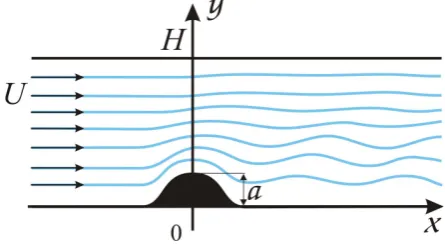
whereρis the fluid density, (u,v) is the fluid velocity vector, p is the pressure and g is the gravity acceleration. It is assumed that the flow domain is bounded from above by rigid lidy=H, whereH is identified with the depth of seawater or troposphere. The topography is represented by the smooth curve y=h(x), so the isolated mountain range is formed by a finite number of hills towering above the ground level y=0 (see Fig. 1). The kinematic boundary conditions at the bottom and the top lid are
v−u∂h ∂x=0
y=h(x), v=0
y=H. (5)
We suppose the absence of internal waves upstream on the left of the mountain range. Upwind flow is presented here by uniform current having constant speedU, so the velocity field should satisfy the condition
(u,v)→(U,0) (x→ −∞) (6)
Fig. 1. Scheme of stratified flow over obstacle.
In this case, the first of the conditions (5) can be replaced under the assumption of a small typical height a of topography by a simplified version of the bottom condition v(x,0)=U dh/dx
which is familiar for the lee wave theory. Using this condition permits us to more easily construct the far-field solution describing wave-train behind obstacle. However, we should preserve here the exact form (5) of the bottom condition in order to obtain the streamline picture precisely at the near field. Keeping this in mind, we introduce the stream functionψ by means ofu=ψy,v= −ψx. Integrating the mass conservation equation (3) implies the dependenceρ=
ρ(ψ ), which can be specified due to the upstream condition (6). Namely, if the upstream uniform flow, defined by the stream function ψ∞(y)=Uy, has known density profile
ρ∞(y)asx→ −∞, then we obtain
ρ(ψ )=ρ∞(ψ/U ). (7)
Now, as it was derived by Dubreil-Jacotin (1935) and Long (1953), eliminating the pressurepfrom the momentum equations (1)–(2) reduces the fully nonlinear Euler system (1)–(4) to equivalent scalar equation
∇2ψ+ρ
0(ψ )
ρ(ψ )
gy−gψ
U + 1 2
|∇ψ|2−U2
=0, (8)
where∇2=∂x2+∂y2is the Laplacian operator andρ0(ψ )=
dρ/dψ(we refer to Yih, 1980 for analytical details). Since the bottom and top lid are supposed to be streamlines, the boundary condition (5) is formulated as follows:
ψ=0
y=h(x), ψ=U H
y=H. (9)
The Dubreil-Jacotin – Long (DJL) equation (8) can be treated for a wide class of density coefficientsρ(ψ )prescribed by the formula (7) with the known function ρ∞. However,
common practice in the lee wave theory is to consider the buoyancy frequencyN,
N2(y)= −gρ
0 ∞(y)
ρ∞(y)
which is assumed to be constant. In this case, it immediately follows that the density ρ∞ depends exponentially on the
height,ρ∞(y)=ρ0exp(−N2y/g), whereρ0is the reference
density attained aty=0.
3 The von Mises transformation of scaled variables
Now, we introduce characteristic scales and control pa-rameters in order to formulate the governing equations in dimensionless form. We select as basic parameters the Boussinesq parameter σ and squared inverse densimetric Froude numberλdefined by the formulae
σ=N
2H
g , λ=
σ gH U2 .
The quantityσ determines the slope of the density profile for a uniformly stratified fluid being at rest and parameterλ qualifies the measure of sub- or super-criticality of upstream flow. Note that λ=F−2, where F =U/(N H ) is the standard Froude number used in most of the papers. On the other hand, there is the relationλ=κ−1, where the scaled frequency κ =N H /U is known as the Long’s number. Finally, we will use dimensionless height of topography α=a/H as a small parameter by applying the perturbation method. Selecting the height H as the length scale and upwind speed U as the velocity scale, we introduce the dimensionless variables as follows:
(x,y,h)=H x,¯ y,¯ h¯
, ψ=U Hψ .¯
In these variables, the shape of the bottom topography can be rewritten asy¯=αh(¯ x), and upstream density profile takes¯
dimensionless formρ∞/ρ0=exp(−σy). Dropping the bar¯ in new variables, we obtain from (8) and (9) the equations
∂2ψ ∂x2+
∂2ψ
∂y2+λ(ψ−y)= 1 2σ ( ∂ψ ∂x 2 + ∂ψ ∂y 2 −1 ) , (10)
ψ=0
y=αh(x), ψ=1
y=1 (11)
with the upstream condition
ψ (x,y)→y (x→ −∞) (12)
Curvilinear shape of lower boundary is the main source of difficulty when solving the problem formulated above. Therefore, we transform the Cartesian coordinates (x,y) in order to simplify the topographic condition (11). Namely, we seek the streamlines in the form y=Y (x,ψ ) with independent (x,ψ)-variables, so the flow domain transforms to the unit strip 0< ψ <1 in the (x, ψ)-plane. This is the von Mises transformation which is well-known in the fluid mechanics, especially in the airfoil theory. Partial derivatives with respect to old and new independent variables are changed by the transformation(x,y)→(x,ψ )as follows:
∂ ∂x → ∂ ∂x− Yx Yψ ∂ ∂ψ, ∂ ∂y → 1 Yψ ∂ ∂ψ.
For instance, first derivatives of both unknown functions ψ (x,y)andY (x,ψ )are coupled by the relations
∂ψ ∂x = −
Yx Yψ , ∂ψ ∂y = 1 Yψ .
As a result, Eq. (10) reduces to the equation
− ∂ ∂x Yx Yψ +1 2 ∂ ∂ψ
1+Yx2 Yψ2
=λ (Y−ψ )+1
2σ
1+Yx2 Yψ2
−1
!
, (13)
and boundary conditions (11) take the simple form
Y (x,0)=αh(x), Y (x,1)=1. (14)
The upstream condition (12) reduces to
Y (x,ψ )→ψ (x→ −∞) (15)
The advantage of the system (13)–(15) is a formulation of equations in a rectangular domain with reserved exact topographic condition at the lineψ=0. However, strong limitations appear while the von Mises transformation suggests all the streamlines to be projectible onto the horizontal levely=0. This condition does not permit step streamlines with overhanging as well as recirculation zones with closed streamlines. Numerous experiments and field observations indicate that vertical jets and zones of reverse flow are ubiquitous in the lee of obstacle of finite amplitude. Therefore, it is clear that the nonlinear model (13)–(15) may serve, in the first place, to simulate topographic flow over the barrier of sufficiently small height.
4 Modelling and results
Approximate analytical solution of the problem (13)–(15) is constructed by the perturbation procedure with small parameter α. Looking for the streamlines Y (x,ψ )=ψ+
αw(x,ψ ) with unknown deviation w, we obtain from Eq. (13) by expanding on powers ofαthe equation
wxx+wψ ψ−σ wψ+λw
=α
wxwψ
x+ 1 2 w
2 x+3w2ψ
ψ
−1
2α σ w 2 x+3w2ψ
+O α2 . (16)
Mises transformation changes the roles of these parameters by settingαto be the dimensionless measure of nonlinearity in the Eq. (16). Thus, we have to solve the linear problem
wxx+wψ ψ−σ wψ+λw=0 (17)
w(x,0)=h(x), w(x,1)=0 (18)
with the upstream condition
w→0 (x→ −∞) . (19)
Equation (17) is well-known in the linear theory of lee waves in the context of using together with the boundary condition on the curvilinear bed (Yih, 1980). However, in the case under consideration, this approximate equation is coupled with the exact condition (18) at the boundary of auxiliary rectangular domain. This distinctive feature provides the model with the flow patterns near the obstacle without loss of accuracy. Spectral problem
φxx+φψ ψ−σ φψ+λφ=0 (0< ψ <1) φ (x,0)=0, φ (x,1)=0
is an important role by solving Eqs. (17)–(19). Discrete normal modes are defined by the eigenfunctions
φn(x,ψ )=eikxeσ ψ/2sinπ nψ (n=1,2,3,...)
which correspond to the eigenvaluesλn=π2n2+k2+σ2/4 with real wave-numberk. Accordingly, parametric range of m-modal lee waves is formed by the values ofλbelonging to the sub-critical domain
π2m2+1
4σ
2< λ < π2(m+1)2+1 4σ
2. (20)
For a givenλsatisfying the condition (20), the set of wave-numbers
kn= q
λ−σ2/4−π2n2 (n=1,...,m) (21) determines the wave-lengths of basic harmonic components which form free wave-train far downstream the mountain range. Note, that neglecting smallσ in (20) leads us back to the known existence condition of lee waves in the case of slight stratification (Yih, 1980).
We use the Dorodnitsyn’s method in order to construct the solution series (the results of Dorodnitsyn’s papers are presented in Kochin et al., 1964). For a given shape of topography h(x), the Fourier solution of Eqs. (17)–(19) determines the elevation of streamlines as follows:
w(x,ψ )=eσ ψ/2
(
y(ψ )h(x)+
∞
X
n=1
wn(x)sinπ nψ )
. (22)
Here the function y(ψ )=sink0(1−ψ )
sink0
(23)
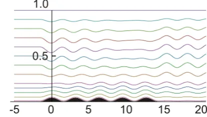
Fig. 2. Lee wave interference with shadow zone over the barrier.
Fig. 3. Isolated wave packets over the barrier.
satisfies the “hydrostatic” equation yψ ψ+k02y =0 with zero mode wave-number k0=
p
λ−σ2/4, and boundary conditionsy(0)=1, y(1)=0 are valid. Infinite sum in the right-hand side of (22) represents the non-hydrostatic part of the solution. The coefficientswnare as follows:
wn(x)= − cn kn
x Z
−∞
sinkn(x−s)h00(s)ds (n=1,...,m)
with the wave-numberskndefined by (21), and
wn(x)= cn 2kn
+∞
Z
−∞
e−kn|x−s|h00(s)ds (n>m+1)
withkn= p
π2n2+σ2/4−λ. In both the formula forw n, real numberscn are the Fourier coefficients of the function y(ψ )from (23) with respect to the basis{sinπ nψ}∞
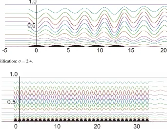
Fig. 4. Lee wave amplification:σ=2.4.
Fig. 5. Separation of wave zones over long sinusoidal topography: forced small-amplitude waves near the bottom (y <0.2) and slow modulated wave-train of moderate amplitude (y >0.2).
fulfilled (Baines, 1995). The dimensionless version of this condition has the formα
√
λ <2, and it is quite true in the case under consideration. The Boussinesq parameterσ is chosen asσ=0.2 except the case of the Fig. 4 whenσ=2.4. The length of the waves forced directly over the topography matches with the period of sinusoidal obstacle. Downstream wave-lengthL=2π/ k1corresponds to the wave-numberk1 from (21).
Figures 2 and 3 compare the interference patterns forced from two different topographies by the same upstream conditions. It is interesting here that the shadow zone arises over the five-bumped barrier. This topography forces no waves directly above the fourth and fifth peaks, but regular periodic wave tail appears beyond the last hill. Figure 3 displays the generation of localized wave packets formed over the eleven-bumped obstacle. Figure 4 illustrates monotone amplification of the wave amplitude by passing the flow over the barrier. Note, that upstream flows found in Figs. 2 and 4 differs only by stratification rate σ and topographies are identical in both the cases. Figure 5 shows an example of irregular interference which appear above the rough sinusoidal barrier composed by thirty three peaks. The wave street placed at the heighty=0.2 seems to be quasi-periodic. The wave amplitude is strongly depressed at this height level despite the upstream flow is very far from the conditions to create critical level.
As expected, wave reflection at the upper boundary did not appear due to small height of the obstacle. However, even for such a smallα, the wave amplification up to the amplitude about ∼0.3 was found by the variation of upstream flow parameters (see Fig. 4), what shows the necessity to take into account nonlinear dispersion effects. The perturbation procedure suggested in this paper allows us to construct higher order approximation inαbased on Eq. (16), this work being in progress now.
5 Conclusions
An analytical model of two-dimensional steady stratified flow over complex topography formed by isolated group of hills is considered. Our method involves asymptotic analysis of the Dubreil-Jacotin – Long equation transformed to the (x,ψ) independent variables, whereψis a stream function. Perturbation procedure uses small dimensionless parameter which characterises the typical height of the obstacle. The wave patterns appearing above the mountain range due to the interference from finite number peaks are calculated. In this paper, we have demonstrated that the flow patterns over the mountain range may be very sensible to the specific shape of topography.
Acknowledgements. We thank the referees for the constructive comments. This work was supported by the RFBR (grant No 09-01-00427), Russian Government (grant No 11.G34.31.0035), Russian Education Department (grant No 2.1.1.4918) and Program RAS (Project No 20.4).
Edited by: E. Pelinovsky
Reviewed by: T. Talipova and another anonymous referee
References
Aguilar, D. A. and Sutherland, B. R.: Internal wave gen-eration from rough topography, Phys. Fluids, 18, 066603, doi:10.1063/1.2214538, 2006.
Aguilar, D., Sutherland, B. R., and Muraki, D. J.: Generation of internal waves over sinusoidal topography, Deep-Sea Res. Pt. II 53, 96–115, 2006.
Baines, P. G.: Topographic Effects in Stratified Flows, Cambridge Univ. Press, New-York, 1995.
Dorodnitsyn, A. A.: Perturbations of airflow caused by the terrain roughness, Proc. Central Geophys. Observatory, 23(6), 3–17, 1938 (in Russian).
Dorodnitsyn, A. A.: Impact of earth relief on the airflow, Proc. Central Forecoast Inst., 21, 3–25, 1950 (in Russian).
Dubreil-Jacotin, M. L.: Compl´ement ´a une note ant´erieure sur les ondes de type permanent dans les liquides h´et´erog´enes, Atti Acad. Lincei Rend. Cl. Sci. Fis. Mat. Nat., 21(6), 344–346, 1935 (in French).
Fraser, N.: Surfing an oil rig, Energy Rev., 20–4 February/March, 1999.
Grimshaw, R. (Ed.): Environmental Stratified Flows, Kluwer, Boston, 2001.
Grimshaw, R. and Smyth, N.: Resonant flow of a stratified fluid over topography, J. Fluid Mech., 169, 429–464, 1986.
Gy¨ure, B. and J´anosi, I. M.: Stratified flow over asymmetric and double bell-shaped obstacles, Dynam. Atmos. Oceans, 37, 155– 170, 2003.
Humi, M.: Long’s equation in terrain following coordinates, Nonlin. Processes Geophys., 16, 533–541, doi:10.5194/npg-16-533-2009, 2009.
Inall, M. E., Shapiro, G. I., and Sherwina, T. J.: Mass transport by nonlinear internal waves on the Malin Shelf, Cont. Shelf Res., 21, 1449–1472, 2001.
Kochin, N. E., Kibel’, I. A., and Rose, N. V.: Theoretical hydromechanics, Wiley, New York, 1964.
Lilly, D. K. and Klemp, J. B.: The effect of terrain shape on non-linear hydrostatic mountain waves, J. Fluid Mech., 95, 241–261, 1979.
Long, R. R.: Some aspects of the flow of stratified fluids, I, A theoritical investigations, Tellus, 5, 42–57, 1953.
Long, R. R.: Some aspects of the flow of stratified fluids, III, Continuos density gradients, Tellus, 7, 341–357, 1955.
Long, R. R.: Finite amplitude disturbances in the flow of inviscid rotating and stratified fluids over an obstacle, Annu. Rev. Fluid Mech., 4, 69–92, 1972.
Lyra, G.: Theorie der stationaren Leewellenstromung in freier atmosphare, Z. Angew. Math. Mech., 23, 1–28, 1943.
Miles, J. W.: Lee waves in a stratified flow, Part 2: Semi-circular obstacle, J. Fluid Mech., 33, 803–814, 1968.
Nappo, C. J.: An introduction to atmospheric gravity waves, Academic Press, San Diego, 2002.
Peltier, W. R. and Clark, T. L.: Nonlinear mountain waves in two and three spatial dimensions, Q. J. Roy. Meteor. Soc., 109, 527– 548, 1983.
Queney, P.: The problem of air flow over mountains: A summary of theoretical studies, B. Am. Meteorol. Soc., 29, 16–26, 1948. Scorer, R. S.: Theory of waves in the lee of mountains, Q. J. Roy.
Meteor. Soc., 75, 41–56, 1949.
Scorer, R. S.: Environmental Aerodynamics, Halsted Press, N.-Y., 1978.
Skopovi, I. and Akylas, T. R.: The role of buoyancy-frequency oscillations in the generation of mountain gravity waves, Theor. Comput. Fluid Dyn., 21(6), 423–433, 2007.
Wurtele, M. G., Sharman, R. D., and Datta, A.: Atmospheric lee waves, Annu. Rev. Fluid Mech., 28, 429–476, 1996.