Fair Value Accounting And Financial
Stability – Based On The Adoption
Of K-IFRS In 2011
Chae Chang Im, Hankuk University of Foreign Studies, South Korea Ahrum Choi, Hong Kong Baptist University, Hong Kong Sungtaek Yim, Hankuk University of Foreign Studies, South Korea
ABSTRACT
Fair value accounting refers to the accounting method which an asset or liability is estimated based on the current market price, so called fair value. Under the fair value accounting, it is more difficult for managers to hide bad information, because the value of an asset or liabilities is re-estimated periodically to reflect the changes in fair value in the market. In this case, firms’ financial stability will be increased. On the other hand, fair value accounting can intensity the volatility of the numbers in the financial statement, which leads to decreases the financial stability. This papers empirically examines the effect of the fair value accounting on the financial stability based on the IFRS adoption in Korea. Using the non-financial firms listed in KOSPI and KOSDAQ from 2000 to 2013, we find that the expansion of fair value accounting increases financial stability. The results support the argument that fair value accounting prohibits managers from hiding bad information, rather it enforces the disclosure of value-relevant information to the investors. The results are consistent with a battery of robustness checks. Thus, the overall results show that the expansion of fair value accounting increase financial stability.
Keywords: Fair Value Accounting; Financial Stability; Crash Risk; Stock Return Volatility; Negative Skewness
1. INTRODUCTION
he role of fair value accounting is in big controversy, especially after financial crisis. Fair value accounting highlights the value-relevant information through mark-to-market accounting. Under the mark-to-market accounting, assets and liabilities are re-estimated periodically to reflect changes in their value and thus accounting information better reflects true underlying performance and financial statements. And due to the mechanism that periodically changes the reported value, it is more difficult for managers to hid bad information to investors under this system. As a results, the information are disclosed to public in a timely manner, works as an early warning mechanisms, which leads to the improvement in firm’s financial stability.
However, there is also a cost in applying fair value accounting. First, the reliability of the accounting number is likely to be distorted since the fair value is estimated by the managers who tend to pursue the strong self-interests. Second, under the fair value accounting, changes in market value can impact on either net income or other comprehensive income. Managers have an opportunistic incentive to transfer the unrealized gains and losses to other comprehensive income, which causes the selective gains trading. Third, the fair value measures sometimes provides less relevant information than amortized (Song and No, 2011). In this respect, fair value accounting is likely to be related to the economic or accounting events that are not directly linked to the firm’s operation activities. According to this view, fair value accounting can impose risks and harm the financial stability.
Despite the competing argument in the relations between fair value accounting and financial stability, there is no direct empirical analysis that examine the effect of fair value accounting and financial stability. Even if there are some empirical studies, they only focused on financial industries (Barth et al., 1995; Veron. 2008) and does not provide implication for non-financial industries.
However, Korea provides a good research setting to test the effect of fair value accounting on crash risk for nonfinancial firms. Since 2011, all listed companies in Korea have to adopt IFRS, which requires all firms to apply extensive fair value accounting in estimating the value of the assets and liabilities. Since previous Korean accounting standard used historical cost accounting system, IFRS adoption could be a good research setting to test the effect of fair value accounting on financial stability, especially for nonfinancial firms. So, the purpose of this paper is to get a comprehensive implication with regard to the effect of fair value accounting on the financial stability. Following prior studies, we measure financial stability using the first, second, and third moment of stock returns: the frequency of crash risk, volatility, and negative skewness respectively. (Chen et al. 2001; DeFond et al. 2015; Hutton et al. 2009; Kim et al. 2010, 2011).
Using the listed firms in KOSPI and KOSDAQ from 2000 to 2013, we find that the expansion of fair value accounting increases financial stability. It supports the argument that fair value accounting prohibits managers from hiding information, rather it enforces the disclosure of value-relevant information to the investors. The results are consistent with a battery of robustness checks. To remove the effect of financial crisis on the financial stability, we examine the separate period, but the main results are not changed. And when we analyze the subsample of firms that adopted IFRS voluntarily, financial stability is also improved after the adoption of IFRS. Thus, the overall results show that the expansion of fair value accounting increase financial stability.
Despite the measurement errors and correlated omitted problems, this paper contributes to the literatures as follows: First, it is the first paper that empirically examines the effect of fair value accounting on financial stability in nonfinancial firms. Second, by comparing the two different accounting system, historical cost accounting versus fair value accounting, it provides practical implication for regulators. Even though fair value accounting can be a double-edged sword, it can work as an instrument for curbing managers’ opportunistic behavior.
The remainder of the paper proceeds as follows: Section 2 describes the institutional backgrounds in Korea and hypothesis development; Section 3 and 4 discusses the research design and data, respectively. Section 5 and 6 shows the main empirical results and sensitivity checks; Finally, Section 7 concludes the paper.
2. HYPOTHESIS DEVELOPMENT
2.1. Fair-Value Accounting in Korea
Korea adopted IFRS (International Financial Reporting Standards) to enhance the accounting transparency in 2011. Adoption of IFRS has influenced various accounting practices in Korea. Korea Accounting Standard Board (KASB) pointed out that the extended application of fair value accounting is one of the key characteristics of IFRS compared to previous accounting standard.1
Before the adoption of IFRS, Korean accounting standard (K-GAAP) is largely based on the cost model in evaluating assets and liabilities. Under the cost model, which emphasize the reliability in accounting information, assets and liabilities are recorded at the initial cost when they are acquired and the value of the assets and liabilities are not changed. Since there is less uncertainty in estimating the value of the assets and liabilities, cost model is better in terms of the reliability.
However, cost-based model does not provide useful information because the recorded value can be far from the market value. Thus, IFRS requires fair value measurement and disclosures to provide more value relevant information. Specifically, all financial assets and liabilities that satisfy certain criteria are estimated based on market value and gain/loss from the financial instruments can be included in net income. IFRS also permits fair-value accounting to nonfinancial assets and liabilities. For example, fair-value accounting can be applied to tangible assets such as land or buildings as well as liabilities including post-employment benefit obligations.
1 As a key difference between IFRS and K-GAAP, KASB mentioned principle-based accounting, fair-value accounting and consolidated financial
2.2. Hypothesis Development
Fair value accounting highlights the value-relevant information through to-market accounting. Under the mark-to-market accounting, assets and liabilities are re-estimated periodically to reflect changes in their value and thus accounting information better reflects true underlying performance and financial statements
However, there is a cost in applying fair value accounting. First, the reliability of the accounting number is likely to be distorted since the fair value is estimated by the managers who tend to pursue the strong self-interests. Second, under the fair value accounting, changes in market value can impact on either net income or other comprehensive income. Managers have an opportunistic incentives to transfer the unrealized gains and losses to other comprehensive income, which causes the selective gains trading2. Third, the amortized cost can be more relevant than the fair value measures since amortized cost is likely to focus on the decision of purchasing, realized income effect and the recovery value (Song and No, 2011). In this respect, fair value accounting is likely to be related to the economic or accounting events that are not directly linked to the firm’s operation activities.
This controversy in fair value accounting is also related to the financial stability. Due to the double sides of fair value accounting, the effect of fair value accounting on the financial stability is also inconclusive. Financial stability means that the stock does not move sharply in the capital market. It sometimes has the opposite concept of crash risk. Financial stability can be considered in three different aspects. First, if the frequency of extreme negative stock returns are too high, the stock is regarded as financially unstable. This is related to the first moment of stock returns. Second aspect is volatility, the second moment of stock returns. If the volatility of the stock is too high, the stock is regarded as financially unstable. Third one is negative return skewness of the firms, which is a third moment of stock returns. If the firm has a disproportionate likelihood of experiencing extreme negative stock returns, financial stability of the firms is considered low.
Some studies provide a hint that fair value accounting has a positive effect on financial stability. Bleck and Liu (2007) show a theoretical rationale for a shift in accounting standards from historic cost accounting to marking to market accounting. According to the paper, marking to market accounting system can better reflect true performance because it provides investors with an early warning mechanisms. Thus, under the fair value accounting, it becomes more difficult for manages to hide bad news. On the other hand, managers have greater opportunities to mask a firm’s true economic performance under historical cost accounting.
Some empirical studies also support the positive role of fair value accounting on the financial stability during the crisis period. During the crisis period, stock returns fluctuate severely. However, Barth et al. (2010) show that fair value accounting is likely to relate little or no role to the financial crisis. Laux et al. (2010) also contradict the contention that fair value accounting has contributed to the year 2008 financial crisis, proposed by the European Commission and U.S. Congress. Instead, they find that there is little evidence as to whether fair value accounting played a role in the U.S banks' problems during the financial crisis.
A recent study by the IMF (2008) delineates pro-cyclical impact of fair value accounting on the capital ratios of banks and seeks potential measures that could mitigate it, which includes expanding the set of liabilities that are mark-to-market and limiting the impact of changes in fair value on the balance sheet via a smoothing mechanism or a circuit breaker. This suggests fair value accounting system mitigate the impact of macroeconomic factors on the financial statement from pro-cyclical market movement. Practically, IMF exhorts the adoption of fair value estimation for the reasons above.
On the other hand, some prior literatures provide evidence that support the negative effect of fair value accounting on the financial stability. For example, banks that have experienced losses from the deficiency of liquidity in crisis period transferred their accounting system from fair value accounting to historical cost accounting (Basel Committee, 2008).
2 Song and Ji (2009) and Song and No (2011) assert that since the gains and losses of valuation from available sales are recognized as capital stocks,
This indicates that the application of the fair value accounting system at financial institutions appears to have weakness and inconsistency in regards to the recent financial crisis in 2008. Under the financial crisis, serious write-offs are required in terms of financial assets at fair value, deteriorating their financial liquidation and credit evaluation. Ultimately, the financial stability is ruined (IIF, 2008)3. In addition, banks recognize the losses at fair value under the economic recession and thus attempt to raise extra capital to maintain their solvency ratio (Veron, 2008) 4. Also, Youngman (2008) asserts that since the financial market is frequently occupied by the market participants’ optimism or pessimism, fair value accounting unintentionally affects the economy and its financial system. Furthermore, fair value accounting intensifies the volatility of the earnings in bank industries (Barth et al., 1995).
Despite the controversy in the relations between fair value accounting and financial stability, there is no direct empirical analysis that examine the effect of fair value accounting and financial stability. Bleck and Liu (2007) show a theoretical comparison between historic cost accounting versus fair value accounting, they did not show any empirical analyses. Even if there are some empirical studies, they only focused on financial industries (Barth et al., 1995; Veron. 2008). The empirical analyses in these studies are largely based on the financial institutions, especially around crisis period, and there is lack of literatures that examines the effect of fair value accounting in nonfinancial companies. International Accounting Standard (IAS) 39, which is directly related to the fair value accounting, contains the standards about the recognition and measurement of financial instruments. That is why many prior literatures deal with financial industries.
However, Korea provides a good research setting to test the effect of fair value accounting on crash risk for nonfinancial firms. Since 2011, all listed companies in Korea have to adopt IFRS, which requires all firms to apply extensive fair value accounting in estimating the value of the assets and liabilities. Since previous Korean accounting standard used historical cost accounting system, IFRS adoption could be a good research setting to test the effect of fair value accounting on the crash risk, especially for nonfinancial firms. Thus, using the Korean data, we test the following hypothesis:
Hypothesis: Ceteris paribus, fair value accounting has no effect on financial stability
3. RESEARCH DESIGN
3.1. Measuring Financial Stability
Financial stability is measured using three variables: crash risk(CRASH), negative skewness(NCSKEW), and stock return volatility(VOL). These three measures are related to the first, second, and third moment of stock return respectively and are inverse measures of financial stability.
3.1.1 Crash Risk (CRASH)
Our first financial stability measure is crash risk, which is widely used in prior studies (Hutton et al. 2009; Kim et al. 2010). To measure crash risk, we first estimate firm-specific weekly returns for each firm and year from the following expanded market model:
𝑟"#=𝛼%+𝛽'"𝑟(,#*'+𝛽+"𝑟",#*'+𝛽,"𝑟(,#+𝛽-"𝑟",#+𝛽."𝑟(,#/'+𝛽0"𝑟",#/'+𝜀",# (1)
3 IIF (2008) reports that the write-off is likely to increase financial risk or liquidity premia under the current fair value accounting system, since the
fair value accounting accelerates further write-downs, margin calls, and the financial volatility. Thus, it is the main cause of the exceeding actual economic losses of many financial instruments.
4 Both IFRS and US GAAP require the disclosure that fair value hierarchy must be attached to the financial statement for financial instruments.
where
𝑟%,# : the return on stock i in week t
𝑟(,# : the return on market index (KOSPI index, KOSDAQ index) in week t
𝜀"# : residual in Equation (1)
We also include the lead and lag terms to allow the non-simultaneous transaction effects (Dimson, 1979). The firm specific weekly return for firm i in week t (𝑊"#) is measured by the natural log of one plus the residual (𝜀"#) in Eq. (1).
We define crash weeks as those weeks during which the stock return experiences weekly returns 3.2 standard deviations below the mean weekly returns over the entire fiscal year. 3.2 standard deviation is equivalent to the 0.1% in the normal distribution. CRASH, which is the first financial stability measure, is defined as an indicator variable that equals to one for a firm-year that experiences one or more firm-specific weekly returns falling 3.2 standard deviations below the mean firm-specific weekly returns over the fiscal year, and zero otherwise. The mean value of CRASH is 0.129, indicating that 12.9% of Korean listed firms, on average, experienced at least one crash event during a given year.
3.1.2 Negative Skewness (NCSKEW)
We measure our second financial stability proxy, NCSKEW, using the negative conditional return skewness (Chen et al. 2001; DeFond et al. 2015; Kim et al. 2011). Main cause of the NCSKEW is the volatility feedback effects (French et al., 1987; Campbell and Hentschel 1992). For example, the large variance of price may cause investors to be more hesitant and cautious, driving the risk premium from the financial market. Furthermore, the increased risk premium is likely to drop the equilibrium price. It will reinforce the impact of the bad news or weaken the impact of the good news. This procedure creates negative skewness (NCSKEW). Thus, stock return with higher negative skewness indicates that the firm’s financial stability is low.
We measure NCSKEW by taking the negative value of the third moment of the firm-specific weekly returns for each sample period and then we divide it by the standard deviation of the firm–specific weekly returns raised to the third power, as shown in the Equation (2) below:
𝑁𝐶𝑆𝐾𝐸𝑊"# = -[𝑛(𝑛 − 1),/+∑𝑊"#,]/ [(𝑛 − 1)(𝑛 − 2)( 𝑊"#
+),/+] (2)
3.1.3 Stock return Volatility (VOL)
Our last measure for financial stability is stock return volatility, VOL. Compare to the previous two measures, VOL does not premise the direction of the stock return. Volatility is calculated as the standard deviation of the firm i’s weekly returns at a given year. Higher volatility indicates that the firm’s stock price changes suddenly and unexpectedly. In other words, volatile stock return means lower financial stability.
3.2 Research Models
We set the model (3) and (4) to show the relation between fair value disclosure and firm’s financial stability as follows:
𝐶𝑅𝐴𝑆𝐻",# 𝑜𝑟 𝑁𝐶𝑆𝐾𝐸𝑊",# 𝑜𝑟 𝑉𝑂𝐿",#
= 𝛼H+ 𝛼'𝐹𝐴𝐼𝑅",#+ 𝛼+𝐷𝑇𝑈𝑅𝑁",#*'+ 𝛼,𝑅𝐸𝑇",#*'+ 𝛼-𝑆𝐼𝑍𝐸",#*' + 𝛼.𝑀𝐵",#*'+ 𝛼0𝐿𝐸𝑉",#*'+ 𝛼R𝑅𝑂𝐴",#*' + 𝛼S𝑁𝐶𝑆𝐾𝐸𝑊"#*'
Where
𝐶𝑅𝐴𝑆𝐻",# : an indicator variable that takes the value of one for a firm-year that experiences one or more
firm-specific weekly returns of firm j at year t
𝑁𝐶𝑆𝐾𝐸𝑊",# : the negative skewness of firm-specific weekly returns over the fiscal year period of firm i at
year t
𝑉𝑂𝐿",# : the standard deviation of the firm i’s weekly returns at year t
𝐷𝑇𝑈𝑅𝑁",#*' : the average of firm-specific weekly trading turnover over the fiscal year period of firm i at
year t-1
𝑆𝐼𝐺𝑀𝐴",#*' : the standard deviation of firm-specific weekly returns over the fiscal year period of firm i at
year t-1
𝑅𝐸𝑇",#*' : the mean of firm-specific weekly returns over the fiscal year t-1
𝑆𝐼𝑍𝐸",#*' : the log of market value of equity of firm i at the beginning of the fiscal year
𝑀𝐵",#*' : the market value of the equity divided by the book value of equity of firm i at the beginning
of the fiscal year
𝐿𝐸𝑉",#*' : the total debts divided by total assets of firm i at the beginning of the fiscal year
𝑅𝑂𝐴",#*' : the income before extraordinary items for fiscal year 5-1 divided by average total assets of firm i
𝑂𝑃𝐴𝑄𝑈𝐸",#*' : the moving sum of the absolute value of discretionary accruals over the last three years (years
t-1, t-2, and t-3) of firm i
We use 𝐶𝑅𝐴𝑆𝐻",# (𝑜𝑟 𝑁𝐶𝑆𝐾𝐸𝑊",# 𝑜𝑟 𝑉𝑂𝐿",# ) as dependent variables to show their relations to the fair value
accounting. 𝐹𝐴𝐼𝑅",# represents our main interest variable which equals to one in the year after the K-IFRS adoption
and 0 otherwise. Based on the prior studies (Chen et al. 2001; Hutton et al. 2009; Kim et al. 2011a, 2011b) we control the following variables that are regarded as the determinants of crash risk:𝐷𝑇𝑈𝑅𝑁#*', 𝑅𝐸𝑇#*', 𝑆𝐼𝑍𝐸#*',
𝑀𝐵#*', 𝐿𝐸𝑉#*', 𝑅𝑂𝐴#*', 𝑁𝐶𝑆𝐾𝐸𝑊#*', 𝑂𝑃𝐴𝑄𝑈𝐸#.
DTURN is the detrended average monthly stock turnover, where turnover is calculated as the monthly trading volume divided by the total number of shares outstanding during the previous fiscal year. DTURN indicates differences in the opinion among the investors, leading to positive (+) coefficient. RET is the average of weekly stock returns for the fiscal-year period. SIZE represents the firm size and expected coefficient is positive, because prior studies show a positive association between firm size and crash risk. MB is the market to book the ratio. Since growth firms are more likely to face negative stock shocks and higher return volatility, we expect MB to be positively related to crash risk. LEV represents the long-term financial stability at time t. Since higher leverage is likely to go through higher financial risk, we expect that LEV to be positively associated to the firm’s crash risk. ROA, which represents the profitability, are expected to have a negative sign because firms with higher profitability have a stable financial condition. 𝑁𝐶𝑆𝐾𝐸𝑊#*' represents the prior period NCSKEW, regarded as one of the determinant of the current financial stability
(Chen et al., 2001). We also suggest OPAQUE as the proxy of financial transparency. Hutton et al. (2009) found that the opacity of financial information is positively related to the firm’s crash risk. Finally, we add the industry dummy (∑INDUS) to the control industry fixed effects.
4. SAMPLE AND DATA
The sample includes all nonfinancial firms that are listed on Korean exchange market, KOSPI and KOSDAQ, from 2000 to 2013. The year 1999 is included when we define the stock crash (CRASH), negative skewness (NCSKEW) and the stock volatility (VOL) since we use the one-year-prior stock weekly returns to estimate these dependent variables. All the other control variables used in the data in the sample period from the year 2000 to 2013.
We excluded firms that belong to financial industry and firms whose fiscal year is not December. Financial institutions are excluded because their financial reporting standard differs from other industries.5 In addition, fair value accounting
5 Before the adoption of K-IFRS in 2011, the reporting system is used to differentiate between general manufacturing firms and financial firms.
and crash risk in the financial industries, especially during the crisis period, are already covered in the prior studies. After deleting observations that have missing values in variables needed to estimate financial stability and other control variables, 16,521 firm-year observations are used in the main analysis. <Table 1> shows summary statistics that used in the main analysis.
Table 1. Summary statistics
Variable Obs. Mean Std. Dev. Min Median Max
NCSKEW 12,988 -0.2571 0.9608 -6.8043 -0.2431 5.3663
CRASH 12,988 0.1290 0.3352 0.0000 0.0000 1.0000
VOL 12,988 7.9306 3.8772 0.0000 7.0921 56.7347
DTURN 12,988 -0.0034 0.0335 -0.9937 -0.0010 0.4949
RET 12,988 0.3386 1.7817 -40.7400 0.2252 71.4300
SIZE 12,988 17.9724 1.5387 12.2691 17.7057 26.1358
MB 12,988 1.3287 6.0562 -89.7471 0.8328 483.8676
LEV 12,988 0.4653 0.3505 0.0086 0.4612 26.4768
ROA 12,988 0.0041 0.2377 -13.0930 0.0298 9.6883
OPAQUE 12,988 0.2792 0.3962 0.0048 0.2014 17.4771
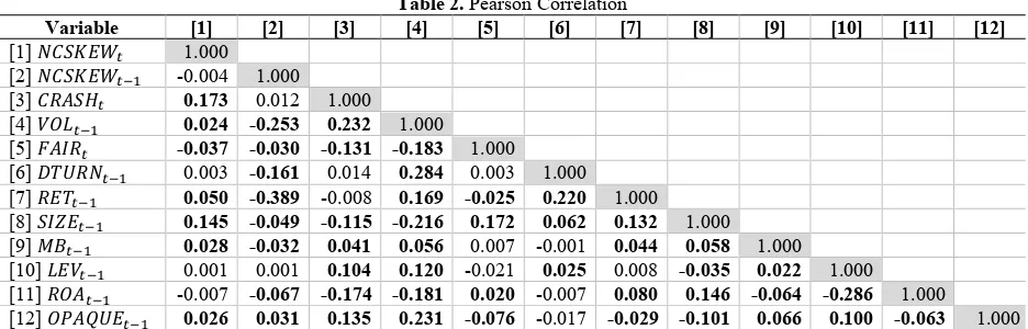
Table 2 shows the correlation among the main variables used in the empirical tests. First, 𝐹𝐴𝐼𝑅# is negatively (-)
related with all the dependent variables (𝐶𝑅𝐴𝑆𝐻#, 𝑁𝐶𝑆𝐾𝐸𝑊#, 𝑉𝑂𝐿#). It means that the expansion of the fair value
accounting is likely to decrease the financial stability. For the control variables, firm size (𝑆𝐼𝑍𝐸#*') and profitability
(𝑅𝑂𝐴#*') are the main causes of the decreased financial stability. On the other hand, the firm’s leverage (𝐿𝐸𝑉#*') and
opacity (𝑂𝑃𝐴𝑄𝑈𝐸#*') are positively (+) related to the financial stability as we expected.
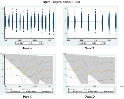
Before exhibiting the main empirical results, we show the trends of the main dependent variables (NCSKEW & VOL) during research period. Panel A of Figure 1 displays the trend of NCSKEW from the year 2000 to 2013. It indicates that the average of NCSKEW differs between period 1 (2000-2010) and 2 (2011-2013). We find that the average value is lower in period 2, compared to period 1. We also attempt to adjust the time period during the year 2006-2013 to show the more recent trends. Panel B of Figure 1 obviously indicates that the average value is lower during period 2, compared to period 1. However, in period 1 from the year 2008 to 2009, an abrupt decrease can be seen, from which we can infer that the effect of financial crisis in the year 2008 affected the financial stability. This is due to the attempt of the regulator trying to stabilize the financial market during the financial crisis and the efforts of the firms to avoid a liquidity risk from the financial market. Panel A and B of Figure 2 show the results of using the VOL, another proxy for a financial stability. These results are similar to the results presented in Figure 1. Thus, we may infer that the financial stability has decreased due to the expansion of the fair value accounting system from IFRS since 2011 in Korea.
Table 2. Pearson Correlation
Variable [1] [2] [3] [4] [5] [6] [7] [8] [9] [10] [11] [12]
[1] 𝑁𝐶𝑆𝐾𝐸𝑊# 1.000
[2] 𝑁𝐶𝑆𝐾𝐸𝑊#*' -0.004 1.000
[3] 𝐶𝑅𝐴𝑆𝐻# 0.173 0.012 1.000
[4] 𝑉𝑂𝐿#*' 0.024 -0.253 0.232 1.000
[5] 𝐹𝐴𝐼𝑅# -0.037 -0.030 -0.131 -0.183 1.000
[6] 𝐷𝑇𝑈𝑅𝑁#*' 0.003 -0.161 0.014 0.284 0.003 1.000
[7] 𝑅𝐸𝑇#*' 0.050 -0.389 -0.008 0.169 -0.025 0.220 1.000
[8] 𝑆𝐼𝑍𝐸#*' 0.145 -0.049 -0.115 -0.216 0.172 0.062 0.132 1.000
[9] 𝑀𝐵#*' 0.028 -0.032 0.041 0.056 0.007 -0.001 0.044 0.058 1.000
[10] 𝐿𝐸𝑉#*' 0.001 0.001 0.104 0.120 -0.021 0.025 0.008 -0.035 0.022 1.000
[11] 𝑅𝑂𝐴#*' -0.007 -0.067 -0.174 -0.181 0.020 -0.007 0.080 0.146 -0.064 -0.286 1.000
[12] 𝑂𝑃𝐴𝑄𝑈𝐸#*' 0.026 0.031 0.135 0.231 -0.076 -0.017 -0.029 -0.101 0.066 0.100 -0.063 1.000
Figure 1. Negative Skewness Trend
Panel A Panel B
Panel C Panel D
In panel A, the dot trend represents the pattern of NCSKEW from 2000 to 2013. The broken line (AVE1) indicates the pattern of NCSKEW from 2000-2010 before the adoption of IFRS in 2011. On the other hand, the solid line (AVE2) represents the pattern of NCSKEW from 2011 to 2013 after the adoption of IFRS in 2011.
In panel B, the dot trend represents the pattern of NCSKEW from 2006 to 2013. The broken line (AVE1) indicates the pattern of NCSKEW from 2006-2010 before the adoption of IFRS in 2011. On the other hand, the solid line (AVE2) represents the pattern of NCSKEW from 2011 to 2013 after the adoption of IFRS in 2011.
In panel C, the solid line trend represents the pattern of NCSKEW’s mean from 2000 to 2013. The long broken line (p25) above the solid line trend indicates the pattern of NCSKEW from 2000 to 2013 within the first quantile (25%). On the other hand, the short broken line (p75) represents the pattern of NCSKEW from 2000 to 2013 within the third quantile (75%).
In Panel D, the solid line trend represents the pattern of NCSKEW’s mean from 2006 to 2013. The long broken line (p25) above the solid line trend indicates the pattern of NCSKEW from 2006 to 2013 within the first quantile (25%). On the other hand, the short broken line (p75) represents the pattern of NCSKEW from 2006 to 2013 within the third quantile (75%).
-5
0
5
2000 2004 2008 2012
NCSKEW AVE1 AVE2
-5
0
5
2006 2008 2010 2012
NCSKEW AVE1 AVE2
-1
.3
-.
8
-.
3
.2
.7
2000 2004 2008 2012
FC FVS
NCSKEW(p25) NCSKEW(mean) NCSKEW(p75)
-1
.1
-.
6
-.
1
.4
.9
2006 2010 2014
FC FVS
Figure 2. Volatility Trend
Panel A Panel B
Panel C Panel D
In panel A, the dot trend represents the pattern of VOL from 2000 to 2013. The broken line (AVE1) indicates the pattern of VOL from 2000-2010 before the adoption of IFRS in 2011. On the other hand, the solid line (AVE2) represents the pattern of VOL from 2011 to 2013 after the adoption of IFRS in 2011.
In panel B, the dot trend represents the pattern of VOL from 2006 to 2013. The broken line (AVE1) indicates the pattern of NCSKEW from 2006-2010 before the adoption of IFRS in 2011. On the other hand, the solid line (AVE2) represents the pattern of VOL from 2011 to 2013 after the adoption of IFRS in 2011.
In panel C, the solid line trend represents the pattern of VOL’s mean from 2000 to 2013. The long broken line (p25) above the solid line trend indicates the pattern of VOL from 2000 to 2013 within the first quantile (25%). On the other hand, the short broken line (p75) represents the pattern of VOL from 2000 to 2013 within the third quantile (75%).
In panel D, the solid line trend represents the pattern of VOL’s mean from 2006 to 2013. The long broken line (p25) above the solid line trend indicates the pattern of VOL from 2006 to 2013 within the first quantile (25%). On the other hand, the short broken line (p75) represents the pattern of VOL from 2006 to 2013 within the third quantile (75%).
5. EMPIRICAL ANALYSIS
Table 3 demonstrates the effect of the expansion of the fair value accounting on the financial stability due to the adoption of IFRS in 2011. First, Column (1) in Table 3 displays a negative coefficient on 𝐹𝐴𝐼𝑅#, indicating that the
adoption of fair value accounting in year 2011 increases negative conditional return skewness. (Coefficient: -0.088, t-value: -4.79). Column (2) also reports a significant negative coefficient of 𝐹𝐴𝐼𝑅# on the firm’s crash risk (Coefficient: -0.602, z-value: -7.93). This indicates that the expansion of fair value accounting from the year 2011 to 2013 decreases crash risk, representing improvement in financial stability. Column (3) reports the result of using VOL as a proxy for financial stability. It also shows a negative relation with FAIR (Coefficient: -0.483, t-value: -8.30).
0
20
40
60
2000 2004 2008 2012
VOL AVE1 AVE2
0
20
40
60
2006 2008 2010 2012
VOL AVE1 AVE2
0
5
10
15
20
2000 2004 2008 2012
FC FVS
VOL(p25) VOL(mean) VOL(p75)
3
6
9
12
2006 2008 2010 2012 FC FVS
All results in Table 3 generally suggest that the expansion of the fair value accounting by the adoption of IFRS improves the firm’s financial instability. The results are consistent with the theoretical argument advocated by Bleck and Liu (2007). Since the fair value accounting provides an early warning mechanisms to the investors, managers have less opportunity to hide bad news in the capital market. In other words, fair value accounting alleviates the firm’s information risk or uncertainty. As a results, the frequency of negative shocks and negative skewness in stock return are reduced. This results are consistent with prior literatures which argues the positive role of fair value accounting in the financial industries. (Barth et al. 2010; Laux et al. 2010)
Table 3. Result of the Expansion of Fair Value System
𝐶𝑅𝐴𝑆𝐻",# 𝑜𝑟 𝑁𝐶𝑆𝐾𝐸𝑊",# 𝑜𝑟 𝑉𝑂𝐿",#
= 𝛼H+ 𝛼'𝐹𝐴𝐼𝑅",#+ 𝛼+𝐷𝑇𝑈𝑅𝑁",#*'+ 𝛼,𝑅𝐸𝑇",#*'+ 𝛼-𝑆𝐼𝑍𝐸",#*'+ 𝛼.𝑀𝐵",#*'+ 𝛼0𝐿𝐸𝑉",#*'
+ 𝛼R𝑅𝑂𝐴",#*' + 𝛼S𝑁𝐶𝑆𝐾𝐸𝑊"#*'+ 𝛼T𝑂𝑃𝐴𝑄𝑈𝐸",#*' + 𝛴𝐼𝑁𝐷𝑈𝑆 + 𝜖"# (3)
Column (1)
Dependent = NCSKEW Dependent = Column (2) CRASH Dependent = Column (3) VOL
Coef. t-value Coef. z-value Coef. t-value
𝐹𝐴𝐼𝑅# -0.088 -4.79 𝐹𝐴𝐼𝑅# -0.602 -7.93 𝐹𝐴𝐼𝑅# -0.483 -8.30
𝑁𝐶𝑆𝐾𝐸𝑊#*' 0.021 2.10 𝑁𝐶𝑆𝐾𝐸𝑊#*' 0.122 3.55 𝑁𝐶𝑆𝐾𝐸𝑊#*' 0.201 6.50
𝐷𝑇𝑈𝑅𝑁#*' -0.718 -2.68 𝐷𝑇𝑈𝑅𝑁#*' -3.131 -4.13 𝐷𝑇𝑈𝑅𝑁#*' -6.037 -7.15
𝑆𝐼𝐺𝑀𝐴#*' 0.010 3.53 𝑆𝐼𝐺𝑀𝐴#*' 0.129 14.51 𝑆𝐼𝐺𝑀𝐴#*' 0.349 38.82
𝑅𝐸𝑇#*' 0.016 3.22 𝑅𝐸𝑇#*' 0.008 0.48 𝑅𝐸𝑇#*' -0.027 -1.73
𝑆𝐼𝑍𝐸#*' 0.120 20.49 𝑆𝐼𝑍𝐸#*' -0.080 -3.42 𝑆𝐼𝑍𝐸#*' -0.397 -21.44
𝑀𝐵#*' 0.002 1.37 𝑀𝐵#*' 0.005 1.37 𝑀𝐵#*' 0.004 0.90 𝐿𝐸𝑉#*' -0.096 -2.33 𝐿𝐸𝑉#*' 0.845 5.93 𝐿𝐸𝑉#*' 1.275 9.85 𝑅𝑂𝐴#*' -0.141 -3.73 𝑅𝑂𝐴#*' -1.029 -6.83 𝑅𝑂𝐴#*' -1.396 -11.77
𝑂𝑃𝐴𝑄𝑈𝐸#*' 0.077 3.57 𝑂𝑃𝐴𝑄𝑈𝐸#*' 0.289 4.00 𝑂𝑃𝐴𝑄𝑈𝐸#*' 0.585 8.65
Indus Included Indus Included Indus Included
Adj_R2 0.035 Pse_R2 0.104 Adj_R2 0.261
No. obs 12,988 No. obs 12,988 No. obs 12,988
Pro>F 0.000 Pro>chi2 0.000 Pro>F 0.000
This table presents results from the regression analyses (H1) of the effect of fair value accounting adoption since 2011 in Korea on financial stability (with the value estimated in NCSKEWE, CRASH and VOL). The fair value accounting system has expanded since 2011. Thus, our main independent variable (FAIR) has a dummy value when the year is 2011, 2012 and 2013, the value has 0; otherwise, 1.
Across all regressions, we take N=12,988 for model (3), (4) and (5) using firm-years observations from 2000 to 2013. We also suggest the results from the regression of CRASH and VOL with similar results with NCSKEW. We suggest coefficient estimates with value, only significant if t-value (z-t-value) > |2|. Column 1 shows the coefficient t-value, wherein the dependent variable is NCSKEW as the proxy of financial stability, with main independent variable FAIR, representing the expansion of fair value accounting system. Column 2 and 3 present the results from similar regression analyses as Column 1 with financial stability estimated with CRASH and VOL. All the variables are defined in the Appendix A.
6. SENSITIVITY TESTS
6.1 Segment Research Periods
To distinguish the effect of the financial crisis occurred in year 2008 from the adoption of K-IFRS effect, we added a separated time dummy variable such as Time2009, Time2010 and Time2011.
𝑁𝐶𝑆𝐾𝐸𝑊",# (𝐶𝑅𝐴𝑆𝐻",#, 𝑉𝑂𝐿",#) = 𝛼H+ 𝛼'𝑃𝐸𝑅𝐼𝑂𝐷1",#+ 𝛼+𝑃𝐸𝑅𝐼𝑂𝐷2",#+ 𝛼,𝑃𝐸𝑅𝐼𝑂𝐷3",#+
𝛼-𝐷𝑇𝑈𝑅𝑁",#*'+ 𝛼.𝑅𝐸𝑇",#*'+ 𝛼0𝑆𝐼𝑍𝐸",#*'+ 𝛼R𝑀𝐵",#*'+ 𝛼S𝐿𝐸𝑉",#*'+ 𝛼T𝑅𝑂𝐴",#*' +
𝛼'H𝑁𝐶𝑆𝐾𝐸𝑊"#*'+ 𝛼''𝑂𝑃𝐴𝑄𝑈𝐸",#*' + 𝛴𝐼𝑁𝐷𝑈𝑆 + 𝜖",# (4)
where
𝑃𝐸𝑅𝐼𝑂𝐷1",# : the time variable of the year 2009 of firm i
𝑃𝐸𝑅𝐼𝑂𝐷2",# : the time variable of the year 2010 of firm i
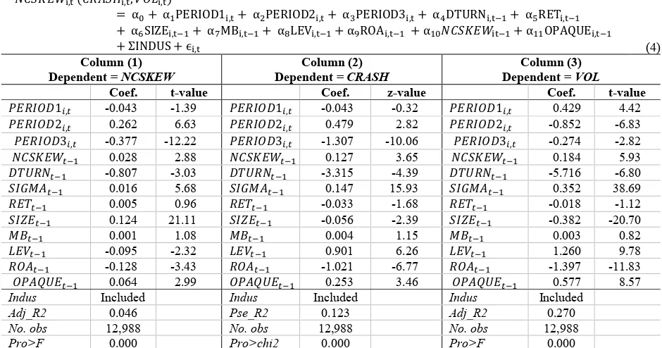
Table 4 shows the sole impact of the financial crisis in the year 2008 on the financial stability. Column (1) provides the result of the separated time trend variables, PERIOD1, PERIOD2 and PERIOD3, with NCSKEW. First, PERIOD1 has a significant negative coefficient (Coefficient: -0.043, t-value: -1.39). This indicates that the financial crash risk is mitigated by the financial regulation, and that the efficient firm’s financial risk managements are possible during the financial crisis. On the other hand, PERIOD2 has a significant positive coefficient (Coefficient: 0.262, t-value: 6.63) so when the impact of the regulation shrinks, it leads the firms to resume investment activities after the financial crisis. As a result, the firm’s crash risk returns to the average level. Finally, PERIOD3, represents the adopted year of IFRS, and reports the significant negative coefficient with NCSKEW (Coefficient: -0.377, t-value: -12.22). This suggests that those two events exclusively affect the financial stability. Column (2) also tests the exclusive effect of the financial crisis and the adoption of IFRS in terms of the financial stability by using the firm’s crash risk measure. PERIOD1 is not significant; however, PERIOD3, representing the expansion of fair value accounting by adoption of IFRS, shows a significant negative coefficient (Coefficient: -1.307, z-value: -10.06). Column (3) suggests that firm’s volatility (VOL) as a proxy of financial stability is related to time trend variables. First, PERIOD1 is positively related to firm’s volatility (Coefficient: 0.429, t-value: 4.42). But PERIOD3 shows negative relation with the firm’s volatility with significance (Coefficient: -0.274, t-value: -2.82). Thus, from the results of <Table 4>, we infer that the effect of financial crisis in the year 2008 and the effect of the adoption of IFRS in 2011 are mutually exclusive on the financial stability.
Table 4. Empirical Result of the Segmented Research Period
𝑁𝐶𝑆𝐾𝐸𝑊[,\ (𝐶𝑅𝐴𝑆𝐻[,\, 𝑉𝑂𝐿[,\)
= αH+ α'PERIOD1[,\+ α+PERIOD2[,\+ α,PERIOD3[,\+ α-DTURN[,\*'+ α.RET[,\*' + α0SIZE[,\*'+ αRMB[,\*'+ αSLEV[,\*'+ αTROA[,\*' + α'H𝑁𝐶𝑆𝐾𝐸𝑊[\*'+ α''OPAQUE[,\*'
+ ΣINDUS + ϵ[,\ (4)
Column (1) Dependent = NCSKEW
Column (2) Dependent = CRASH
Column (3) Dependent = VOL
Coef. t-value Coef. z-value Coef. t-value
𝑃𝐸𝑅𝐼𝑂𝐷1",# -0.043 -1.39 𝑃𝐸𝑅𝐼𝑂𝐷1",# -0.043 -0.32 𝑃𝐸𝑅𝐼𝑂𝐷1",# 0.429 4.42
𝑃𝐸𝑅𝐼𝑂𝐷2",# 0.262 6.63 𝑃𝐸𝑅𝐼𝑂𝐷2",# 0.479 2.82 𝑃𝐸𝑅𝐼𝑂𝐷2",# -0.852 -6.83
𝑃𝐸𝑅𝐼𝑂𝐷3",# -0.377 -12.22 𝑃𝐸𝑅𝐼𝑂𝐷3",# -1.307 -10.06 𝑃𝐸𝑅𝐼𝑂𝐷3",# -0.274 -2.82
𝑁𝐶𝑆𝐾𝐸𝑊#*' 0.028 2.88 𝑁𝐶𝑆𝐾𝐸𝑊#*' 0.127 3.65 𝑁𝐶𝑆𝐾𝐸𝑊#*' 0.184 5.93
𝐷𝑇𝑈𝑅𝑁#*' -0.807 -3.03 𝐷𝑇𝑈𝑅𝑁#*' -3.315 -4.39 𝐷𝑇𝑈𝑅𝑁#*' -5.716 -6.80
𝑆𝐼𝐺𝑀𝐴#*' 0.016 5.68 𝑆𝐼𝐺𝑀𝐴#*' 0.147 15.93 𝑆𝐼𝐺𝑀𝐴#*' 0.352 38.69
𝑅𝐸𝑇#*' 0.005 0.96 𝑅𝐸𝑇#*' -0.033 -1.68 𝑅𝐸𝑇#*' -0.018 -1.12 𝑆𝐼𝑍𝐸#*' 0.124 21.11 𝑆𝐼𝑍𝐸#*' -0.056 -2.39 𝑆𝐼𝑍𝐸#*' -0.382 -20.70
𝑀𝐵#*' 0.001 1.08 𝑀𝐵#*' 0.004 1.15 𝑀𝐵#*' 0.003 0.82
𝐿𝐸𝑉#*' -0.095 -2.32 𝐿𝐸𝑉#*' 0.901 6.26 𝐿𝐸𝑉#*' 1.260 9.78
𝑅𝑂𝐴#*' -0.128 -3.43 𝑅𝑂𝐴#*' -1.021 -6.77 𝑅𝑂𝐴#*' -1.397 -11.83
𝑂𝑃𝐴𝑄𝑈𝐸#*' 0.064 2.99 𝑂𝑃𝐴𝑄𝑈𝐸#*' 0.253 3.46 𝑂𝑃𝐴𝑄𝑈𝐸#*' 0.577 8.57
Indus Included Indus Included Indus Included
Adj_R2 0.046 Pse_R2 0.123 Adj_R2 0.270
No. obs 12,988 No. obs 12,988 No. obs 12,988
Pro>F 0.000 Pro>chi2 0.000 Pro>F 0.000
This table shows the results of sensitivity test to identify the pure effect on financial stability (with the value estimated with NCSKEWE, CRASH
and VOL) of the effect of the expansion of fair value accounting system from the effect of financial crisis in 2008 in the regression model (6), (7) and (8). The fair value accounting system has expanded since 2011, thus our main independent variable (FAIR) has a dummy value when the year is 2011, 2012 and 2013, the value has 0; otherwise, 1.
Across all the regressions, we take N=12,988 for model (6), (7) and (8) using firm-years observations from 2000 to 2013. We also suggest the results from the regression of CRASH and VOL with similar results with CRASH. We suggest coefficient estimates with t-value, only significant if t-value (z-value)> |2|. Column 1 shows the coefficient value, wherein the dependent variable is NCSKEW as the proxy of financial stability, with main independent variable FAIR, representing the expansion of fair value accounting system. Column 2 and 3 present the results from similar regression analyses as Column 1 with financial stability estimated with CRASH and VOL. All the variables are defined in the Appendix A.
6.2 Comparison between the Impacts on Financial Stability by Industry Types
Table 5. Industry Categories
Industries N of Obs Percent Cumulative
[1] Construction 559 3.38% 3.38% [4] Wholesale and Retail 1,342 8.12% 11.51% [5] Communication 373 2.26% 13.76% [6] Non-Metal Manufacturing 1,740 10.53% 24.30% [7] Consumer Manufacturing 1,911 11.57% 35.86% [9] Electronics Manufacturing 3,026 18.32% 54.18% [10] Expert Service 1,568 9.49% 63.67% [11] Detailed Manufacturing 2,741 16.59% 80.26% [12] Publication, Media, Broadcasting and Information Services 718 4.35% 84.61% [13] Chemical Manufacturing 2,543 15.39% 100%
Total 16,521 100% 100%
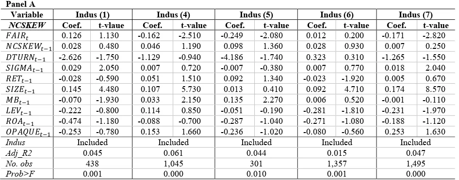
Table 6 shows the results that examine the effect of fair value accounting on financial stability of each industry. The results generally support that FAIR is negatively (-) related to NCSKEW (IndusN (4), (5), (7), (9), (10), and (13)). We can infer that the expansion of fair value accounting is likely to increase financial stability. Thus, we conclude that the expansion of fair value accounting by adopting K-IFRS in 2011 affects financial stability even in the test with individual industries.
Table 6. Comparison of the Impact on the Financial Stability by Individual Industry Types Panel A
Variable Indus (1) Indus (4) Indus (5) Indus (6) Indus (7)
NCSKEW Coef. t-vlaue Coef. t-value Coef. t-value Coef. t-value Coef. t-value
𝐹𝐴𝐼𝑅# 0.126 1.130 -0.162 -2.510 -0.249 -2.080 0.012 0.200 -0.171 -2.820
𝑁𝐶𝑆𝐾𝐸𝑊#*' 0.028 0.480 0.046 1.190 0.098 1.360 0.028 0.930 0.007 0.250
𝐷𝑇𝑈𝑅𝑁#*' -2.626 -1.750 -1.129 -0.940 -4.186 -1.740 0.323 0.310 -1.265 -1.550
𝑆𝐼𝐺𝑀𝐴#*' 0.029 2.050 0.007 0.720 -0.007 -0.380 0.007 0.770 0.018 2.040
𝑅𝐸𝑇#*' -0.028 -0.590 0.051 1.510 0.092 1.340 -0.023 -1.920 0.005 0.670
𝑆𝐼𝑍𝐸#*' 0.145 4.480 0.107 5.730 0.013 0.410 0.092 4.710 0.174 8.570
𝑀𝐵#*' -0.070 -1.930 0.033 2.150 0.135 2.270 0.006 0.520 -0.001 -0.110
𝐿𝐸𝑉#*' -0.222 -0.800 0.114 0.850 -0.051 -0.190 -0.281 -1.810 -0.231 -1.970
𝑅𝑂𝐴#*' -0.474 -1.180 -0.088 -0.700 -0.287 -1.040 -0.271 -1.080 -0.188 -1.120
𝑂𝑃𝐴𝑄𝑈𝐸#*' -0.253 -0.780 0.153 1.660 -0.236 -1.020 -0.080 -0.560 0.253 1.630
Indus Included Included Included Included Included
Adj_R2 0.045 0.061 0.044 0.015 0.047
No. obs 438 1,045 301 1,357 1,495
Prob>F 0.001 0.000 0.010 0.001 0.000
(Table 6 continued)
Panel B
Variable Indus (9) Indus (10) Indus (11) Indus (12) Indus (13)
NCSKEW Coef. t-value Coef. t-value Coef. t-value Coef. t-value Coef. t-value
𝐹𝐴𝐼𝑅# -0.097 -2.390 -0.101 -1.790 -0.043 -0.980 -0.079 -0.970 -0.089 -1.810
𝑁𝐶𝑆𝐾𝐸𝑊#*' 0.021 0.820 0.070 2.030 0.068 2.460 0.029 0.540 0.085 3.040
𝐷𝑇𝑈𝑅𝑁#*' -0.332 -0.650 -1.157 -1.260 -1.573 -2.310 -1.401 -1.480 -2.236 -2.760
𝑆𝐼𝐺𝑀𝐴#*' 0.002 0.280 -0.010 -1.160 0.020 2.500 0.002 0.130 -0.004 -0.470
𝑅𝐸𝑇#*' 0.080 4.040 0.094 3.170 0.084 3.500 0.154 3.620 0.118 4.170
𝑆𝐼𝑍𝐸#*' 0.138 9.170 0.099 5.770 0.093 6.510 0.187 4.790 0.085 4.950
𝑀𝐵#*' -0.001 -0.440 0.001 0.260 0.001 0.700 0.003 0.120 0.027 2.250
𝐿𝐸𝑉#*' 0.041 0.440 0.044 0.370 -0.113 -1.040 0.075 0.350 -0.106 -0.890
𝑅𝑂𝐴#*' -0.189 -2.870 -0.051 -0.590 0.034 0.230 -0.373 -2.140 -0.130 -0.540
𝑂𝑃𝐴𝑄𝑈𝐸#*' 0.075 2.600 0.114 2.430 0.196 2.340 0.120 0.680 0.022 0.150
Indus Included Included Included Included Included
Adj_R2 0.052 0.048 0.037 0.088 0.036
No. obs 2,420 1,372 2,140 577 1,978
Prob>F 0.000 0.000 0.000 0.000 0.000
This table suggests the results of sensitivity test to identify the sole effect on financial stability (with the value estimated in NCSKEW) of the effect of the expansion of the fair value accounting system in the regression model (3), (4) and (5) by each industry. The fair value accounting system has expanded since 2011, and thus our main independent variable (FAIR) has a dummy value when the year is 2011, 2012 and 2013, the value has 0; otherwise, 1.
Across all the regressions, we take N=16,521 by using firm-years observations from 2000 to 2013. We suggest coefficient estimates with t-value (z-value), only significant if t-value > |2|. Column 1 shows the coefficient value, wherein the dependent variable is NCSKEW as the proxy of financial stability, with main independent variable FAIR, representing the expansion of fair value accounting system. Column 2 and 3 present the results from similar regression analyses as Column 1 with financial stability estimated with CRASH and VOL. All the variables are defined in the Appendix A.
6.3 Early Adoption of K-IFRS on the Financial Stability
Previous results show the effect of mandatory adoption of K-IFRS on the financial stability. However, several firms voluntarily adopted K-IFRS earlier than 2011. Early adopters may have different characteristics that are related to the financial stability compared to the other firms. Thus, we test the effect of the early adoption of K-IFRS on the financial stability using the following regression model:6
𝑁𝐶𝑆𝐾𝐸𝑊",#(𝐶𝑅𝐴𝑆𝐻 & 𝑉𝑂𝐿) = 𝛼H+ 𝛼'𝐸𝐴𝐷𝑂𝑃",#+ 𝛼+𝐷𝑇𝑈𝑅𝑁",#*'+ 𝛼,𝑅𝐸𝑇",#*'+ 𝛼-𝑆𝐼𝑍𝐸",#*'+
𝛼.𝑀𝐵",#*'+ 𝛼0𝐿𝐸𝑉",#*'+ 𝛼R𝑅𝑂𝐴",#*' + 𝛼S𝑁𝐶𝑆𝐾𝐸𝑊"#*'+ 𝛼T𝑂𝑃𝐴𝑄𝑈𝐸",#*' + 𝛴𝐼𝑁𝐷𝑈𝑆 + 𝜖"# (5)
where
𝐸𝐴𝐷𝑂𝑃",#: firms that early adopts the K-IFRS
Table 7. Empirical Result of the Early Adoption Firms
𝑁𝐶𝑆𝐾𝐸𝑊[,\(𝐶𝑅𝐴𝑆𝐻 & 𝑉𝑂𝐿)
= αH+ α'EADOP[,\+ α+DTURN[,\*'+ α,RET[,\*'+ α-SIZE[,\*'+ α.MB[,\*'+ α0LEV[,\*'
+ αRROA[,\*' + αS𝑁𝐶𝑆𝐾𝐸𝑊[\*'+ αTOPAQUE[,\*' + ΣINDUS + ϵ[\ (5)
Column (1)
Dependent = NCSKEW Dependent = Column (2) CRASH Dependent = Column (3) VOL NCSKEW Coef. t-value CRASH Coef. z-value VOL Coef. t-value
𝐸𝐴𝐷𝑂𝑃# -0.089 -4.84 𝐸𝐴𝐷𝑂𝑃# -0.612 -8.06 𝐸𝐴𝐷𝑂𝑃# -0.489 -8.42
𝑁𝐶𝑆𝐾𝐸𝑊#*' 0.021 2.09 𝑁𝐶𝑆𝐾𝐸𝑊#*' 0.122 3.54 𝑁𝐶𝑆𝐾𝐸𝑊#*' 0.201 6.50
𝐷𝑇𝑈𝑅𝑁#*' -0.716 -2.67 𝐷𝑇𝑈𝑅𝑁#*' -3.116 -4.11 𝐷𝑇𝑈𝑅𝑁#*' -6.027 -7.14
𝑆𝐼𝐺𝑀𝐴#*' 0.010 3.53 𝑆𝐼𝐺𝑀𝐴#*' 0.129 14.50 𝑆𝐼𝐺𝑀𝐴#*' 0.349 38.83
𝑅𝐸𝑇#*' 0.016 3.21 𝑅𝐸𝑇#*' 0.008 0.46 𝑅𝐸𝑇#*' -0.028 -1.74
𝑆𝐼𝑍𝐸#*' 0.121 20.51 𝑆𝐼𝑍𝐸#*' -0.078 -3.36 𝑆𝐼𝑍𝐸#*' -0.396 -21.35
𝑀𝐵#*' 0.002 1.36 𝑀𝐵#*' 0.005 1.36 𝑀𝐵#*' 0.004 0.90
𝐿𝐸𝑉#*' -0.096 -2.33 𝐿𝐸𝑉#*' 0.843 5.92 𝐿𝐸𝑉#*' 1.274 9.84
𝑅𝑂𝐴#*' -0.141 -3.75 𝑅𝑂𝐴#*' -1.034 -6.87 𝑅𝑂𝐴#*' -1.398 -11.79
𝑂𝑃𝐴𝑄𝑈𝐸#*' 0.077 3.57 𝑂𝑃𝐴𝑄𝑈𝐸#*' 0.290 4.01 𝑂𝑃𝐴𝑄𝑈𝐸#*' 0.586 8.66
Indus Included Indus Included Indus Included
Adj_R2 0.035 Pse_R2 0.104 Adj_R2 0.262
No. obs 12,988 No. obs 12,988 No. obs 12,988
Prob>F 0.000 Pro>chi2 0.000 Prob>F 0.000
This table suggests the results of the test to identify the pure effect of the early adoption of IFRS on financial stability (with the value estimated with NCSKEWE, CRASH and VOL) of the effect of the expansion of fair value accounting system in the regression model (9), (10) and (11). The fair value accounting system has expanded since 2011, but many firms are allowed to adopt the earlier IFRS system, and thus we attempt to segment the effect of the early adoption. To test the effect of the early adoption, we set the additional model (9), (10) and (11), and our main independent variable (EADOP) has a dummy value when the firm adopts IFRS earlier than others.
Across all the regressions, we take N=12,988 for model (9), (10) and (11) using firm-years observations from 2000 to 2013. We also suggest the results from the regression of CRASH and VOL with similar results with NCAKEW. We suggest coefficient estimates with t-value, only significant if t-value (z-value) > |2|. Column 1 shows the coefficient value, wherein the dependent variable is NCSKEW as the proxy of financial stability, with main independent variable EADOP, representing the expansion of fair value accounting system. Column 2 and 3 present the results from similar regression analyses as Column 1 with financial stability estimated with CRASH and VOL. All the variables are defined in the Appendix A.
Table 7 shows the results of the effect of the early adoption of K-IFRS on the financial stability. First, column (1) in Table 7 suggests the negative sign (-) between financial stability (NCSKEW) and the fair value accounting before 2011 (Coefficient: -0.0089, t-value: -4.84). This indicates that the early adoption enables companies to enjoy enhanced financial stability through the fair value accounting. Second, column (2) in Table 7 suggests similar results. Early adopters have less likelihood of crash risk. It can also be inferred that the fair value accounting is likely to lead to enhancement of the financial stability (Coefficient: -0.612, z-value: -8.06). Finally, column (3) in Table 7 shows that the early adoption firms are negatively (-) related with volatility (Coefficient: -0.489, t-value: -8.42). The results in Table 7 generally supports that fair value accounting decreases the firm’s crash risk as well as firm’s entire volatility risk. Thus, we contend that the expansion of fair value accounting improves financial stability.
7. CONCLUSION
To test the effect of fair value accounting on financial stability, we use Korean data. Korea provides a good research setting to test the effect of fair value accounting on crash risk for nonfinancial firms. Since 2011, all listed companies in Korea have to adopt IFRS, which requires all firms to apply extensive fair value accounting in estimating the value of the assets and liabilities. Since previous Korean accounting standard used historical cost accounting system, IFRS adoption could be a good research setting to test the effect of fair value accounting on financial stability, especially for nonfinancial firms.
Using the listed firms in KOSPI and KOSDAQ from 2000 to 2013, we find that the expansion of fair value accounting increases financial stability. It supports the argument that fair value accounting prohibits managers from hiding information, rather it enforces the disclosure of value-relevant information to the investors. The results are consistent with a battery of robustness checks. To remove the effect of financial crisis on the financial stability, we examine the separate period, but the main results are not changed. And when we analyze the subsample of firms that adopted IFRS voluntarily, financial stability is also improved after the adoption of IFRS. Thus, the overall results show that the expansion of fair value accounting increase financial stability.
Despite the measurement errors and correlated omitted problems, this paper contributes to the literatures as follows: First, it is the first paper that empirically examines the effect of fair value accounting on financial stability in nonfinancial firms. Second, by comparing the two different accounting system, historical cost accounting versus fair value accounting, it provides practical implication for regulators. Even though fair value accounting can be a double-edged sword, it can work as an instrument for curbing managers’ opportunistic behavior.
AUTHOR BIOGRAPHIES
Chaechang Im (1st Author) is a Ph.D. of Hankuk University of Foreign Studies. 107, Imun-ro, Dongdaemun-gu, Seoul, 02450, South Korea. E-mail: imcee@naver.com.
Ahrum Choi (corresponding author), Ph.D., is an assistant professor at Hong Kong Baptist University. WLB 615,
34 Renfrew Road, Kowloon, Hong Kong. E-mail: archoi@hkbu.edu.hk.
Sungtaek Yim (Co-Author) is a Ph.D. of Hankuk University of Foreign Studies. 107, Imun-ro, Dongdaemun-gu, Seoul, 02450, South Korea. E-mail: yst17@paran.com.
REFERENCES
Aboody, D., M. E. Barth, & R. Kasznik. (2004). Firms' Voluntary Recognition of Stock-based Compensation Expense. Journal of Accounting Research 42: 123-50.
Ahmed, A., E. Kilic, & G. Lobo. (2006). Does Recognition versus Disclosure Matter? Evidence from Value-relevance of Banks’ Recognized and Disclosed Derivative Financial Instruments. TheAccounting Review 81: 567-88.
Barth, M. & W. Landsman. (2010). How did Financial Reporting Contribute to the Financial Crisis?, The European Accounting Review 19: 399-423.
Barth, M. E., Landsman, W. R. & Wahlen, J. M. (1995). Fair Value Accounting: Effects on Banks’ Earnings Volatility, Regulatory Capital, and Value of Contractual Cash Flows, Journal of Banking & Finance, 19: 577–605.
Basel Committee on Banking Supervision. (2008). Fair Value Measurement and Modeling: An Assessment of Challenges and Lessons Learned from the Market Stress. Bank for International Settlements
Benmelech, Efraim, & Jennifer Dlugosz. (2009). The Credit Rating Crisis. NBER Working Paper 15045.
Campbell, J.Y., Hentschel, L., 1992. No News is Good News: An Asymmetric Model of Changing Volatility in Stock Returns.
Journal of Financial Economics 31: 281–318.
Chen, J., H. Hong, & J. C. Stein. (2001). Forecasting Crashes: Trading Volume, Past Returns, and Conditional Skewness in Stock Prices. Journal of Financial Economics 61: 345-381.
Dimson, E., (1979). Risk Measurement When Shares are Subject to Infrequent Trading. Journal of Financial Economics 7: 197– 227.
French, K.R., Schwert, G.W., & Stambaugh, R.F. (1987). Expected Stock Returns and Volatility. Journal of Financial Economics 19: 3-29.
Hutton, A. P., A. J. Marcus, & H. Tehranian. (2009). Opaque Financial Reports, R2, and Crash Risk. Journal of Financial Economics 94: 67-86.
Conduct and Best Practice Recommendations.
International Monetary Fund (IMF). (2008). Global Financial Stability Report. Jeffrey, G. (2008). Mark market debate down as a draw. The Bottom Line
Ji, H. M. & Song, I. M. (2009). Earnings Management Using the Selective Disposal of Available-for-Sale Securities. Korean Accounting Review 34: 1-26. [Printed in Korean]
Jin, L., & S. C. Myers. 2006. R2 around the World: New Theory and New Tests. Journal of Financial Economics 79: 257-292. Kim, J., & L. Zhang. (2010). Does Accounting Conservatism Reduce Stock Price Crash Risk? Firm-level Evidence. Working
paper.
Kim, J. O. (2011). The Effect of K-IFRS Adoption on Financial Reporting: Evidence from Early Adopted Listed Company.
Korea Accounting Information Journal 29 (2): 345-368. [Printed in Korean]
Kim, J., Y. Li, & L. Zhang. (2011). Corporate Tax Avoidance and Stock Price Crash Risk: Firm-level Analysis. Journal of Financial Economics 100: 639-662.
Laux, C. (2010). Did Fair-value Accounting Contribute to the Financial Crisis? Journal of Economic Perspectives 24 (1): 93-118. Lee, J. H., J. Y., Cho & Im, C. C. (2014). The Impact of Reporting Quality on Crash Risks in the Korean Stock Market, Korean
Accounting Review 39 (2): 361-394. [Printed in Korean]
Li K., Morck R., Yang F., & Yeung B. (2004). Firm-specific Variation and Openness in Emerging Markets. Review of Economics and Statistics 86: 658–669.
Magnan, M. L. (2009).Fair Value Accounting and the Financial Crisis: Messenger or Contributor? Accounting Perspectives 8 (3): 189-213.
McFarland, J., & J. Partridge. (2008). Mark-to-market Accounting Rules Fuel Debate. Globe and Mail. Report on Business.
Penman, S. H. (2007). Financial Reporting Quality: Is Fair Value a Plus or a Minus? Accounting & Business Research (Wolters Kluwer UK). Special Issue: 33-43.
Piotroski, J. D., & Roulstone, D.T. (2004). The Influence of Analysts, Institutional Investors and Insiders on the Incorporation of Market, Industry and Firm-specific Information into Stock Prices. Accounting Review 79: 1119–1151.
Roll, R. (1988). R2. Journal of Finance 43(1): 541-566.
Ryan, S. G. (2008). Accounting in and for the Subprime Crisis. The Accounting Review 83 (6):1605-1638.
Securities and Exchange Commission (SEC). (2008). Report and Recommendations Pursuant to Section 133 of the Emergency Economic Stabilization Act of 2008: Study on Mark-to-market Accounting. Office of the Chief Accountant, Division of Corporation Finance, Washington, DC.
Song, I. M., & H. S, No. (2011). IFRS and Fair Value Evaluation. KIF Finance Report from Korea Institute of Finance (3): 1-103. [Printed in Korean]
Venkatachalam, M. (1996). Value Relevance of Banks’ Derivatives Disclosures. Journal of Accounting and Economics 22 (1-3): 327-55.
APPENDIX A
Variable Definitions
Category Definition
Dependent Variables
NCSKEW the negative skewness of firm-specific weekly returns over the fiscal year period
CRASH
an indicator variable that takes the value of one for a year that experiences one or more firm-specific weekly returns falling 3.2 standard deviations below the mean firm-firm-specific weekly returns over the fiscal year, with 3.2 chosen to generate frequencies of 0.1% in the normal distribution during the fiscal year period, and zero, otherwise.
VOL The standard deviation of firm i weekly returns at year t
Control Variables
DTURN the average of firm-specific weekly trading turnover over the fiscal year period of firm j at year t-1
SIGMA the standard deviation of firm-specific weekly returns over the fiscal year period of firm j at year t-1
RET the mean of firm-specific weekly returns over the fiscal year period, times 100
SIZE the log value of market value of firm j at year t-1
MB the market value of the equity divided by the book value of equity of firm j at year t-1
LEV total debts divided by total assets of firm j at year t-1
ROA income divided by average total assets of firm j at year t-1
OPAQUE the moving sum of the absolute value of discretionary accruals over the last three years (years t-1, t-2, and t-3). (Hutton et al. 2009)
Variables for Sensitivity Tests
TIME2009 the time variable of 2009
TIME2010 the time variable of 2010
TIME2011 the time variable of 2011
APPENDIX B
Early Adoption Firms of K-IFRS from 2009 to 2010
Panel A
KOSPI Transition Day Industry
KT&G 2008.1.1 Manufacturing STX PANOCEAN 2008.1.1 Transportation Pulmuone Holdings 2008.1.1 Manufacturing EAGON 2008.1.1 Manufacturing COSMO CHEMICAL 2008.1.1 Manufacturing YOUGJIN Pharmaceutical 2008.1.1 Manufacturing LG 2009.1.1 Expert Service LG Display 2009.1.1 Manufacturing LG Life Sciences 2009.1.1 Manufacturing LG Household & Health Care 2009.1.1 Manufacturing LG Electronics 2009.1.1 Manufacturing LG Innotek 2009.1.1 Manufacturing LG U+ 2009.1.1 Communication LG Chem 2009.1.1 Manufacturing Samsung Electronics 2009.1.1 Manufacturing Samsung SDI 2009.1.1 Manufacturing KOREA FLANGE 2009.1.1 Manufacturing GⅡR 2009.1.1 Expert Service
Sum of KOSPI firms 18 Firms
Panel B
KOSDAQ Transition Day Industry
PAPER COREA 2008.1.1 Manufacturing INSUN ENT 2008.1.1 Wastewater Treatment DISPLAYTECH 2008.1.1 Manufacturing Palytech 2008.1.1 Manufacturing CUBIC KOREA 2008.1.1 Manufacturing ECOENERGY Holdings 2008.1.1 Manufacturing GIKO&ROOTIZ 2008.1.1 Manufacturing KOOKJE ELECTRIC KOREA 2008.4.1 Manufacturing NEXCON Technology 2009.1.1 Manufacturing DBK 2009.1.1 Manufacturing ENTER TECH 2009.1.1 Manufacturing UJU ELECTRONICS 2009.1.1 Manufacturing EUGENE 2009.1.1 Manufacturing CAVAC 2009.1.1 Manufacturing
Sum of KOSDAQ firms 14 Firms