197
Assessing The Adequacy Of Split-Plot Design
Models
David, I. J., Asiribo, O. E., Dikko, H. G.
Abstract: This paper assesses the adequacy of model fit of the split-plot design models that is the whole plot (WP) sub design model with WP error and the split-plot (SP) sub design model with SP error using the four measures of adequacy of fit for the WP and SP sub designs proposed by Almimi et al.
[3] which are the R2, R2-Adjusted, Prediction Error Sum of Square (PRESS) and R2-Prediction statistics and we proposed five other methods which are the Modeling Efficiency (MEF), Resistant Coefficient of Determination (r2r), Mean Square Error (MSE), Mean Square Error Prediction (MSEP) and
Adequate Precision (AP) statistics. A 2(1+3) replicated two-level SP design and 31 x 42 replicated mixed level SP design were used for computing the measures of model adequacy of fit for each WP and SP sub design models. These measures describe the predictive performance of each WP and SP sub design models.
Key Words: AP, MEF, MSE, MSEP, Model Adequacy, PRESS, R2, R2-Adjusted, R2-Prediction, r2r, SP error, WP error
————————————————————
1 INTRODUCTION
Experiments are performed by investigators in virtually all fields of enquiry, usually to discover something about a particular process or system. Literarily, an experiment is a test. A designed experiment is a test or series of tests in which purposeful changes are made to the input variables of a process or system so that we may observe and identify the reasons for changes in the output responses [15]. The split-plot experimental design has a model with two experimental errors and the adequacy of the model can be diagnosed for its fitness, using methods such as the coefficient of determination (R2), adjusted coefficient of determination (R2 - Adjusted), prediction error sum of squares (PRESS), mean bias, graphical approach, etc. The manner in which the measures of
R2, R2 - Adjusted, PRESS, etc are obtained from a design with one type of error in its model is quite different from that of the split-plot design with two types of errors in its model, which are whole plot or main plot error and the split-plot or sub-plot error. The calculation of these measures should be for both the main plot error and the split-plot error due to the assumption that the whole-plot errors are independent and identically distributed as N (0, σ2w), and the split-plot errors are independent and
identically distributed as N (0, σ2
), which are mutually independent. These are, guaranteed by the system of randomization in split-plot experimental design [3]. Almimi et al. [3] stated that although R2 is a useful measure of goodness of fit, it has some limitations [15]: R2 can increase by adding terms to the model, the magnitude of R2 depends on the range of variability in the regressor variable, and R2 does not measure the magnitude of the slope of the regression line.
Nonetheless, the use of the least-square method to derive a linear regression of observed on model-predicted values for model evaluation has little interest since the predicted value is useless in evaluating the mathematical model; therefore, the
R2 is irrelevant since one does not intend to make predictions from the fitted line [13]. Then R2 is weakly increasing in the number of regressors in the model as such, R2 models with different numbers of independent variables. This conforms to the statement by [3] that the limitations about R2 mentioned by [15] call for the use of alternative measures. He further stated that the R2 – adjusted is preferred to R2 because its value only increases if a variable that is being added to the model reduces the residual mean square. Hence, unlike R2, R2 – adjusted does not increase if irrelevant terms are being added to the model. Masoud and Rahim [11] stated that when outliers occur in a data the assumption of normally distributed errors is violated and reduces the performance of the linear regression models. Further they stated that detecting outliers is much easier than deciding what to do with them because after detecting, the investigator should consider whether the outliers are recording errors. They advised that after these cases are detected they should never be blindly deleted and the investigator should analyze the full data set including the outliers as well as the data set after the outliers have been removed (either by deleting the cases or the variables that contain the outliers). Kvalseth [8] proposed the use of resistant coefficient of determination (rr
2
), which uses the medians instead of the means and results in a coefficient that is highly resistant to outliers or extreme data points. Almimi et al. [3] stated that the prediction error sum of squares, PRESS and
R2- prediction which are useful measures of model adequacy were proposed by [1], [2], is used to evaluate the performance of the model in predicting the responses in new and future experiments. Moreover, PRESS is very useful when comparing models because a model with a small value of PRESS is generally better than a model with a large value of PRESS. Similarly, R2-Prediction, which is based on PRESS, is
a measure of the predictive performance of a model. Tedeschi [17] presented the modelling efficiency statistic (MEF), in which he stated that the method is similar to ρ, which is interpreted as the proportion of variation explained by the fitted line whereas the MEF statistic is the proportion of variation explained by the line Y = f(X1, . . , Xp). He further stated that the statistic has been extensively used in hydrology models, but can certainly be used in biological models. He concluded that in a perfect fit, both the ρ (correlation coefficient) and the ————————————————
David, I. J. is currently a PhD student of Statistics in Department of Mathematics, Ahmadu Bello University, Zaria-Nigeria. PH- +2348060581391. Email: [email protected]
Asiribo, O. E. is a Professor of Statistics, Department of Mathematics, Ahmadu Bello University, Zaria-Nigeria. PH- +8033526707.
MEF would result in a value equal to one and that the upper bound of MEF is one and the (theoretical) lower bound of MEF is negative infinity. Loague and Green [10] stated that if MEF is lower than zero; the model predicted values are worse than the observed mean. The MEF statistic may be used as a good indicator of goodness of fit [12]. Tedeschi [17] stated that the mean square error (MSE) and the mean square error of prediction (MSEP) are probably the most common and reliable estimate to assess the precision and measure the predictive accuracy of a model respectively. Tedeschi [17] stated that the MSE assesses the precision of the fitted linear regression using the difference between observed values (Yi) and regression-predicted values (Ŷi). While MSEP consist of the difference between observed values (Yi) and model – predicted values (f (Xi,…,Xp)i) rather than regression-predicted value. Sergio and Joan [16] stated that like variance, MSE has the disadvantage of heavily weighting outliers. They said it is because of the squaring of each term, which effectively weights large errors more heavily than small ones. This property, undesirable in many applications, has led researchers to use alternatives such as the mean absolute error, or those based on the median. Some drawbacks of the MSE and MSEP analysis are notable. Mitchell and Sheehy [14] stated that the MSEP (or its root) removes the negative sign and weights the deviation by their squares, thus giving more influence to larger data points, and does not provide any information about model precision. Tedeschi [17] stated that the MSEP estimate is a reliable measure of model accuracy. Nonetheless, the reliability will decrease as n decreases. Therefore, the estimate of MSEP variance has an important role. Tedeschi [17] further stated that a different scenario arises when the model parameters are adjusted to the data set; the real MSEP will be underestimated because the model will reproduce more closely the data that have been modeled than it would for the entire population of interest. A simple and easy approach to check model adequacy between two (or more) models is computing the MSEP of each model and choosing the one with smaller MSEP estimates. Wallach and Goffinet (1989) presented a different approach that makes use of the difference in MSEP (∆MSEP) values between two models. They stated that if the estimated difference (∆MSEP) is positive then model g(Z1,…,Zk)i is preferred, while if ∆MSEP is negative then model f(X1,…,Xp)i is preferred since it has the smaller MSEP estimate.
n
Z
Z
g
Y
X
X
f
Y
S
n i i k i i p i
1 2 1 21
,...,
)
(
,...,
)
(
Montgomery [15] presented and discussed the adequate precision (AP) statistic which is computed by dividing the difference between the maximum predicted (max Ŷi) response
and the minimum predicted (min Ŷi) response by the average
standard deviation of all predicted responses. He stated that large values of this quantity are desirable and values that exceed four (AP > 4) usually indicate that the model will give reasonable performance in prediction. This paper discussed potential weakness in some of the methods used in checking adequacy of models that uses the mean which is not resistant to outliers and their strength if the median is used instead of the mean.
2 METHODOLOGY
Nine methods and their procedures to compute model adequacy of fit from a split-plot design as discussed in the literature are explored. Four out of the nine methods were used, being applied by Almimi et al. [3] in both the replicated and unreplicated split-plot design. However, we introduced the application of the remaining four out of which we proposed the use of difference in mean square error (∆MSE) values between two models that is the whole plot and split-plot models and the method proposed by Wallach and Goffinet [18]: difference in mean square error prediction (∆MSEP). In this research paper, we only considered the replicated split-plot design.
2.1 Procedure for Computing Model Adequacy of Fit from Split-Plot Design
Detailed procedures for computing the measures of model adequacy of fit from split-plot design for R2, R2 – Adjusted,
PRESS and R2-Prediction are been given by Almimi et al. [3]. However, we presented procedures for the other introduced measures for model adequacy of fit from split-plot design. The introduced measures are modeling efficiency statistic (MEF), resistant coefficient of determination (R2r), difference in mean
square error (∆MSE), difference in mean square error prediction (∆MSEP) and adequate precision (AP).
2.1.1 MEF (Modeling Efficiency) Statistic
1. From the WP sub-design, subtract the model-predicted values (f(X1,…,Xp)i) from the observed
values (Yi), take the summation and square. Divide
the value obtained by the total sum of squares (SSTotal) for the WP sub-design and subtract the value
obtained from one to obtain the MEF for the WP sub-design model.
MEFWP=
n i WP i ni i WP
p i
Y
Y
X
X
f
Y
1 2 ) ( 1 2 ) ( 1,...,
1
(1)2. Use the ANOVA column for the SP sub-design, subtract the model-predicted values (f(X1,…,Xp)i) from
the observed values (Yi), take the summation and
square. Divide the value obtained by the total sum of squares (SSTotal) and subtract the value obtained from
one to obtain the MEF for the SP sub-design model.
MEFSP =
n i SP i n i SP i p iY
Y
X
X
f
Y
1 2 ) ( 1 2 ) ( 1,...,
1
(2)2.1.2
r
r2 (Resistant Coefficient of Determination)199
2. Obtain the absolute difference of the mean value of the WP observed values from the WP observed
values (|Yi (wp) -
Y
(wp)|) and obtain its median(Med|Yi (wp) -
Y
(wp)|).3. Divide (Med|ei (wp)|) by (Med|Yi (wp) -
Y
(wp)|) square theresult obtained and subtract from 1 to obtain
r
r2 .2 ) (wp r
r
=
2 1 11
WP i n i WP i n iY
Y
M
e
M
(3)4. For the SP sub-design, the
r
r2 is calculated using the absolute SP residual (|ei (sp)|) and obtain its median (Med|ei (sp)|).5. Obtain the absolute difference of the mean value of the SP observed values from the SP observed values
(|Yi (sp) -
Y
(sp)|) and obtain its median (Med|Yi (sp) -(sp)
Y
|).6. Divide (Med|ei (sp)|) by (Med|Yi (sp) -
Y
(sp)|) square theresult obtained and subtract from 1 to obtain
r
r2 .2 ) (sp r
r
=
2 1 11
SP i n i SP i n iY
Y
M
e
M
(4)2.1.3 ∆MSE (Difference in Mean Square Error) and ∆MSEP (Difference in Mean Square Error Prediction)
1. Use the ANOVA column of the WP sub-design with the complete whole plot factors (i.e. significant and insignificant factors) to obtain the residual sum of square (SSResidual) and divide by (n-2) to obtain the
MSE for WP as follows:
MSEWP =
( ) ) ( Re2
WP WP sidualn
SS
(5)2. Use the ANOVA column of the SP sub-design with the complete split-plot factors (i.e. significant and insignificant factors) to obtain the residual sum of square (SSResidual) and divide by (n-2) to obtain the
MSE for SP as follows:
MSESP =
( ) ) ( Re2
SP SP sidualn
SS
(6)3. Obtain the difference between the MSEWP and MSESP as follows:
∆MSE(wp, sp) = MSEwp – MSEsp (7)
4. Use the ANOVA column of the WP sub-design to obtain the residual sum of square (SSResidual) and
divide by (n) to obtain the MSEP for WP as follows:
MSEPWP =
( ) ) ( Re WP WP sidualn
SS
(8)5. Use the ANOVA column of the SP sub-design to obtain the residual sum of square (SSResidual) and
divide by (n) to obtain the MSE for SP as follows:
MSEPSP =
( ) ) ( Re SP SP sidualn
SS
(9)6. Obtain the difference between the MSEPWP and MSEPSP as follows:
∆MSEP(wp, sp) = MSEPwp – MSEPsp (10)
2.1.4 Adequate Precision (AP)
1. Obtain the fitted values corresponding to the whole plot sub model.
2. Select the maximum predicted response (Max Ŷ) and minimum predicted response (Mini Ŷ) corresponding to the whole plot.
3. Obtain their difference (Max Ŷ – Mini Ŷ).
4. Divide the estimated difference (Max Ŷ– Mini Ŷ) by the average standard deviation of all predicted response corresponding to the whole plot
APwp =
WP Y WP
n
S
Y
Min
Y
Max
)
(
)
ˆ
ˆ
(
ˆ
(11)5. Obtain the fitted values corresponding to the split-plot sub model.
6. Select the maximum predicted response (Max Ŷ) and minimum predicted response (Mini Ŷ) corresponding to the split plot.
7. Obtain their difference (Max Ŷ – Mini Ŷ).
8. Divide the estimated difference (Max Ŷ– Mini Ŷ) by the average standard deviation of all predicted response corresponding to the split plot
APsp =
SP Y SP
n
S
Y
Min
Y
Max
)
(
)
ˆ
ˆ
(
ˆ
(12)2.1.5 Whole Plot and Split-Plot Residuals Calculation
Almimi et al. [3] presented the procedure in calculating the whole plot (WP) and split-plot (SP) residuals, the steps are been given as follows:
2. Subtract the fitted values from the response values to obtain the residuals.
3. To calculate the WP residuals, average the residuals that correspond to the runs in each WP. Now, all the runs within a WP have the same WP residual.
4. To calculate the SP residuals, subtract the WP residuals obtained in step 3 from the residuals obtained in step 2 for all the runs in the design.
3.0 ANALYSIS AND DISCUSSION OF RESULTS
The data used for illustrations for the various methods discussed in this paper are of two sets where the first set is one of the data used by Almimi et al. [3] which is a 2(1+3) replicated two-level split-plot design data. The data consist of four factors each at two levels, the WP sub design is made of one factor (Z) and the remaining three factors (A, B and C) are for the SP sub designwhile the second set of data is a 31 x 42 replicated mixed level split-plot design data on the effect of four nitrogen fertilizer levels on the yield of four varieties of rice at three irrigation levels.
3.1 Presentation and Interpretation of Results for the 2(1+3) Replicated Two-Level Split-Plot Design
After we applied all the procedures for the reviewed methods and proposed methods for checking model fitness from a 2(1+3) replicated two-level split-plot design. Below are the results.
Table 1: ANOVA for the 2(1+3) Replicated Two-Level Split-Plot Design
ANOVA for the WP Sub Design
Source DF SS MS F P-Value
Model 1 59.13 59.13 2.94 0.228
Z 1 59.13 59.13 2.94 0.228
Error 2 40.17 20.08
Total 3 99.30
ANOVA for the SP Sub Design
Source DF SS MS F P-value
Model 5 2136.9
4
427.38
8 155.8 0.0001
A 1 597.72 597.72 217.9
2 0.0001
B 1 1226.3
6
1226.3 6
447.0
9 0.0001
ZA 1 14.72 14.72 5.37 0.030
ZB 1 285.01 285.01 103.9
0 0.0001
AB 1 13.13 13.13 4.79 0.039
Error 23 63.08 2.743
Total 28 2200.0
2
Source: Author’s computation
Table 2: Summary of the Results for the Four Measures of Model Adequacy of Fit for the 2(1+3) Replicated
Two-Level Split-Plot Design by Almimi et al. [3]
Whole Plot Sub Design Subplot Sub Design
R2WP 0.595
2
SP
R
0.971R2WP -Adjusted 0.393 R 2
SP –Adjusted 0.965
PRESSWP 40.293 PRESSSP 63.866
R2WP –
Predicted 0.594
R2SP –
Predicted 0.971
Source: Author’s computation
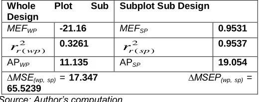
Table 3: Summary of the Results for the Four Proposed Measures of Model Adequacy of Fit for the 2(1+3) Replicated
Two-Level Split-Plot Design by Almimi et al. [3]
Whole Plot Sub Design
Subplot Sub Design
MEFWP -21.16 MEFSP 0.9531
2 ) (wp r
r
0.3261 2) (sp r
r
0.9537APWP 11.135 APSP 19.054
∆MSE(wp, sp) = 17.347 ∆MSEP(wp, sp) =
65.5239
Source: Author’s computation
Table 1 above present the ANOVA table for the WP sub design significant effects and the SP sub design significant effects while table 2 present results for the four measures of model adequacy of fit from a 2(1+3) replicated two level split-plot design presented by [3] and table 3 present the results for the four introduced measures for this paper for model adequacy of fit from a 2(1+3) replicated two level split-plot design presented by [3]. The measures proposed by [3] and those we proposed provide some notable difference though conclusion is the same. The R2, adj- R2, and pred-R2values for the WP and SP sub design model are (0.595 and 0.971), (0.393 and 0.965)
and (0.594 and 0.971) respectively. The
r
r2and MEF values for the WP and SP sub design model are (0.3261 and 0.9537) and (-21.6 and 0.9531) respectively. We observed that the R2and pred-R2 values for the WP sub design model is about 60% but the adj-R2 value for the WP sub design model is 39%
comparing both values the difference is large and this is an indication that the R2 and pred-R2 values could be misleading but for the SP sub design model the difference between the R2
and pred-R2 value of 97% and adj- R2 value of 96.5% is small, this shows that for the SP sub design model R2 and pred-R2
are reliable as the adj- R2. Comparing this values with the 2
r
r
and MEF values we observed that ther
r2value for the WP sub design model of 32.6% is even smaller than theadj-R2 value of 39% this is an indication that the
r
r2is not affected by outliers in the data so its value is not influenced by it and the R2 and pred-R2 are not to be relied upon. Likewise, the negative value of the MEF is a clear indication for worse predictive values by the WP sub design effects because thevalue is less than zero. The values of
r
r2(95.37%) and MEF201 and pred-R2 values (97%) and adj-R2 value (96.5%) this is
another indication that the
r
r2 is not affected by outliers andis more reliable likewise the MEF value is similar to the
r
r2 value. The PRESS value for the WP sub design model is smaller compared to the SP sub design model PRESS value which is large indicating that the WP sub design model fit well in predicting new responses compared to the SP sub design model but this is not in agreement with other measures of fit which indicates that the SP sub design model is adequately fit compared to the WP sub design model. Likewise, the APvalues for the WP and SP sub design model are large because they exceed four but the SP sub design model value is larger. The PRESS and AP values can be misleading as that of the R2 and pred-R2 values because we observed that a small value of PRESS or large value of AP does not really tell that the model fit adequately besides the PRESS is worse because there is no bench mark or cut point to say a PRESS value is small enough or too large to say a model fit adequately or worse while the AP value could be that, it is affected by outliers that is why we observed an AP value greater than four in the WP sub design model when it is been
observed by other measures (
r
r2, adj-R2 and MEF) values indicated that the WP sub design model is not adequately fit.3.2 Presentation and Interpretation of Results for the 31x42 Replicated Mixed Level Split-Plot Design
In this section we applied all the reviewed methods and proposed methods for checking model fitness from a 31 x 42 replicated mixed level split-plot design. Below are the results.
Table 4: ANOVA for the 31x42 Replicated Mixed Level Split-Plot Design
ANOVA for the WP Sub Design Sourc
e Df SS MS F
P-Value Model 5 860.93
1 172.19 15.75
I 2 742.92
2 371.46 33.99 0.0001
V 3 118.009 39.34 3.6 0.034
Error 18 196.69
9 10.93
Total 23 1057.6 3
ANOVA for the SP Sub Design Sourc
e Df SS MS F
P-value Model 18 542.68 30.15 8.469
N 3 198.16 66.05 18.56 0.0001
I*N 6 156.62 26.10 7.34 0.0001
V*N 9 187.90 20.88 5.87 0.0001
Error 54 192.17 3.56
Total 72 734.85
Source: Author’s computation
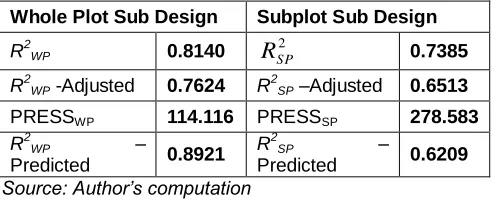
Table 5: Summary of the Results for the Four Measures of Model Adequacy of Fit for the 31x42 Replicated Mixed
Level Split-Plot Design
Whole Plot Sub Design Subplot Sub Design
R2WP 0.8140
2
SP
R
0.7385R2WP -Adjusted 0.7624 R 2
SP –Adjusted 0.6513
PRESSWP 114.116 PRESSSP 278.583
R2WP –
Predicted 0.8921
R2SP –
Predicted 0.6209
Source: Author’s computation
Table 6: Summary of the Results for the Four Proposed Measures of Model Adequacy of Fit for the 31 X 42 Replicated
Mixed Level Split-Plot Design
Whole Plot Sub
Design Subplot Sub Design
MEFWP 0.9229 MEFSP 0.7307
2 ) (wp r
r
0.8824r
r2(sp) 0.8477APWP 31.8567 APSP 41.1480
∆MSE(wp, sp) = 7.37 ∆MSEP(wp, sp) = -1.1558
Source: Author’s computation
Table 4 above present the ANOVA table for the WP sub design significant effects and the SP sub design significant effects while table 5 above present the results for the four measures (used by [3]) of model adequacy of fit from a 31 x 42 replicated mixed level split-plot design and table 6 above present the results for the four introduced measures for the research paper of model adequacy of fit from a 31 x 42 replicated two level split-plot designs. The measures proposed by [3] and those we proposed provides some notable differences though conclusion is the same. The R2, adj- R2, and pred-R2 values for the WP and SP sub design model are (0.8140 and 0.7385), (0.7624 and 0.6513) and (0.8921 and 0.6209) respectively.
The
r
r2and MEF values for the WP and SP sub design model are (0.8824 and 0.8477) and (0.9229 and 0.7307) respectively. We observed that the pred-R2value for the WP is greater than the R2 WP and the pred-R2 value for SP sub design model is less than that of the R2 value for the SP sub design model, these differences could be due to the presence of outliers in the data. The adj-R2 value for the WP sub design model is lower than that of the R2 and pred-R2 and its SP sub design model value is less than the R2 value but slightly above the pred-R2 value this shows its ability to withstand unnecessary increment when a factor is removed or added from a model but it is not free from the effect of outliers.Comparing this values with the
r
r2and MEF values weobserved that the
r
r2value for the WP sub design model of 88.24% is greater than the R2 and the adj-R2 values but there is no much difference with the WP pred- R2 value while theMEF value for the WP sub design model is greater than all the
model. There is no much difference in
r
r2value for both the WP and SP sub design models and base on these values fromthe
r
r2we could say that the WP and SP sub design models predict well the observed values because both values explainlarge variability in the data. This shows that the
r
r2is not affected by outliers in the data. The PRESS statistic value for the WP sub design model support the claim that the WP is adequate for prediction but, the AP value do not support the claim rather it support the SP sub design model to be more adequately precise in navigating its design space though both AP values for the WP sub design and SP sub design are far greater than four and this could be its inability of withstanding outliers or extreme data point.4 CONCLUSION
The results obtained from the 2(1+3) replicated two-level
split-plot design showed that the
r
r2result is unbiased because its value is not affected by outliers, its SP sub design model value is high but not as high as the R2, adj-R2 and pred-R2 values which are affected by outliers as sited in the literature. The results from the methods applied on the second data (31 x 42 replicated mixed level split-plot design) showed that the WP sub design model attained high values of R2, adj-R2, pred-R2,MEF and
r
r2with negative value of ΔMSEP but the AP and ΔMSE values showed that the SP sub design model have a better predictive Precision and from our observation ther
r2 value for the WP sub design model (0.8824) is not adequately larger than the SP sub design model value (0.8477). Based on these results we cannot completely say that the WP sub design model is better than the SP sub design model rather they are operating in the same rate. This is an indication that the other measures of model adequacy of model fit could be missleading due to none resistance to outliers, unecessary increase or reduction of values due to introduction of a variable or variables into the model or removal of a variable or variables from the model. Based on our observations we recommend the following for assessing the adequacy of model fit from SP designs and checking the performance of two or more models either for present or future use.1. Measures of adequacy of fit of models that uses the mean could be misleading because their magnitudes are not consistently related to the accuracy of prediction, that is, where accuracy is defined as the degree to which model-predicted observations approach the magnitudes of their observed counterparts [19]. So, care should be taking in using measures that uses the mean.
2. We recommend the use of robust objective functions, which are based on the median instead of the mean because the resistant coefficient of determination
2
r
r
which uses the median shows that its reliability is adequate due to its ability of withstanding outliers or extreme data points.3. The ΔMSE and the ΔMSEP values could be
questionable because as N samples become smaller their results becomes biased, so, we recommend that large sample size should be used, if sample size is
small then they should not be considered as reliable measures for model adequacy of fit.
4. We recommend also that the ΔMSE is not an
adequate measure of model fit for SP designs and should not be relied upon because it is often expected that the WP sub design model will always have the largest MSE compared to the MSE of the SP sub design model only in rare and special cases where the reverse is the case because the SP design usually sacrifices precision in estimating the average effects of the treatments assigned to WP sub design by improving the precision for comparing the average effects of treatments assigned to SP sub design. Hence, we recommend the use of ΔMSE for assessing the precision of regression models.
5. We also recommended that the PRESS and AP statistic could be misleading because they don’t have reliabel bench mark or point interval for recommending a best PRESS or AP value. Although, the AP value is desirable or best when its value is > 4 [15] but we observed that we obtained AP values that are adequately > 4 for both the WP sub design and SP sub design models for both data.
Finally, it is our hope that this research paper presents the strength and fault of each methods explored either as a review or introduction to assessing adequacy of model fit from split-plot designs with objective basis for model selection by researchers in the field of Statistics, Mathematics, Econometrics, Agronomy, Biological Sciences, etc.
REFERENCES
[1]. Allen, D. M. (1971). Mean Square Error of Prediction as a Criterion for Selecting Variables. Technometrics 13(3): 469-475.
[2]. Allen, D. M. (1971). The Relationship between Variable Selection and Data Augmentation and a Method for Prediction. Technometrics 16(1): 125-127.
[3]. Almini, A. A., Kulahci, M. and Montgomery, D. C. (2006). Checking the Adequacy of fit of Models from split-plot Designs. Journal of Quality Technology 38: 58 – 190.
[4]. Berger, J. O. (1985). Statistical Decision Theory and Bayesian Analysis, 2nd ed. New York: Springer-Verlag. PP. 60.
[5]. DeGroot, M. H. (1980). Probability and Statistics. 2nd ed. Addison-Wesley.
[6]. Dent, J. B. and Blackie, M. J. (1979). Systems Simulation in Agriculture. Applied Science, London.
[7]. Draper, N. R. and Smith, H. (1998). Applied Regression Analysis. Wiley-Interscience. ISBN 0-417-17082-8.
[8]. Kavalseth, T. O. (1985). Cautionary Note about R2. The American Statistician 39: 279 – 285.
203 MR1639875 (
http://www.ams.org/mathscinet-getitem?mr=1639875). ISBN 0-387-98502-6.
[10]. Loague, K. and Green, R. E. (1991). statistical and Graphical Methods for Evaluating Solute Transport Models: Overview and Application. Journal of Contaminant Hydrology 7: 51-73.
[11]. Masoud, Y. and Rahim, M. (2010). The Effect of Outliers on Robust and Resistant Coefficient of Determination in the Linear Regression Models. International Journal of Academic Research 2(3): 133-138.
[12]. Mayer, D.G. and Butler, D.G. (1993). Statistical Validation. Ecological Modeling 68: 21 - 32.
[13]. Mitchell, P. L. (1997). Misuse of Regression for Empirical Validation of Models. Agricultural Systems 54: 313-326.
[14]. Mitchell, P. L. and Sheehy, J. E. (1997). Comparison of Predictions and observations to assess Model Performance: A Method of Empirical Validation. Kluwer Academic Publishers, Boston. MA, PP. 437-451.
[15]. Montgomery, D. C. (2005). Design and Analysis of Experiments, 5th ed. John Wiley and Sons New York, PP. 76-104 and 392 – 422.
[16]. Sergio, B. and Joan, C. (2001). Oriented Principal Component Analysis for Large margin Classifiers. Neural Networks 14(10): 1447-1461.
[17]. Tedeschi, L. O. (2006). Assessment of the Adequacy of Mathematical Models. Agricultural systems 89: 225-247.
[18]. Wallach, D. and Goffinet, B. (1989). Mean Squared Error of Prediction as a Criterion for Evaluating and Comparing System Models. Ecological Modeling 44: 299-306.