www.nat-hazards-earth-syst-sci.net/14/1341/2014/ doi:10.5194/nhess-14-1341-2014
© Author(s) 2014. CC Attribution 3.0 License.
Subsidence activity maps derived from DInSAR data:
Orihuela case study
M. P. Sanabria1,3, C. Guardiola-Albert2, R. Tomás3,4, G. Herrera2,3, A. Prieto1, H. Sánchez1, and S. Tessitore2,5
1Geohazards InSAR laboratory and Modelling group, Infrastructures and services Department, Geological Survey of Spain, Rios Rosas 23, 28003 Madrid, Spain
2Geohazards InSAR laboratory and Modelling group, Geosciences Department, Geological Survey of Spain, Alenza 1, 28003 Madrid, Spain
3Unidad Asociada de investigación IGME-UA de movimientos del terreno mediante interferometría radar (UNIRAD), Universidad de Alicante, P.O. Box 99, 03080 Alicante, Spain
4Departamento de Ingeniería Civil, Escuela Politécnica Superior, Universidad de Alicante, P.O. Box 99, 03080 Alicante, Spain
5Department of Earth Sciences, Environment and Resources, Federico II University of Naples, Naples, Italy Correspondence to: M. P. Sanabria (m.sanabria@igme.es)
Received: 11 September 2013 – Published in Nat. Hazards Earth Syst. Sci. Discuss.: 8 October 2013 Revised: – – Accepted: 13 April 2014 – Published: 27 May 2014
Abstract. A new methodology is proposed to produce
sub-sidence activity maps based on the geostatistical analysis of persistent scatterer interferometry (PSI) data. PSI displace-ment measuredisplace-ments are interpolated based on conditional Sequential Gaussian Simulation (SGS) to calculate multiple equiprobable realizations of subsidence. The result from this process is a series of interpolated subsidence values, with an estimation of the spatial variability and a confidence level on the interpolation. These maps complement the PSI displace-ment map, improving the identification of wide subsiding ar-eas at a regional scale. At a local scale, they can be used to identify buildings susceptible to suffer subsidence related damages. In order to do so, it is necessary to calculate the maximum differential settlement and the maximum angular distortion for each building of the study area. Based on PSI-derived parameters those buildings in which the serviceabil-ity limit state has been exceeded, and where in situ foren-sic analysis should be made, can be automatically identified. This methodology has been tested in the city of Orihuela (SE Spain) for the study of historical buildings damaged during the last two decades by subsidence due to aquifer overex-ploitation. The qualitative evaluation of the results from the methodology carried out in buildings where damages have been reported shows a success rate of 100 %.
1 Introduction
in-formation on the temporal evolution of the ground displace-ment (Arnaud et al., 2003; Berardino et al., 2002, Ferretti et al., 2001, 2011; Mora et al., 2003; Prati et al., 2010; Sowter et al., 2013). These techniques have been validated for subsi-dence monitoring with measurements obtained using classi-cal survey techniques by Herrera et al. (2009a, b), Hung et al. (2011), and Raucoules et al. (2009). These authors computed
±1 mm year−1 and±5 mm errors for the average displace-ment rate and cumulated displacedisplace-ment values along the line of sight (LOS), respectively.
Mostly, A-DInSAR techniques have been applied to mon-itor wide areas affected by ground surface movements asso-ciated with groundwater changes (e.g. Galloway et al., 2007; Heleno et al., 2011; Raspini et al., 2012; Stramondo et al., 2008; Tomás et al., 2010, 2014). Fewer works use these tech-niques to monitor singular urban structures and infrastruc-tures and indicate their usefulness as a prevention tool (Karila et al., 2005; Bru et al., 2010; Herrera et al., 2010; Cigna et al., 2011, 2012; Tapete et al., 2012; Arangio et al., 2013; Sousa et al., 2013). Some authors (Cascini et al., 2007; Tomás et al., 2012) go further, and apply geotechnical criteria to A-DInSAR techniques in order to identify buildings where set-tlement induced damages could occur.
This work focuses on the utility of A-DInSAR tech-niques to monitor and characterize the phenomenon of sub-sidence both regionally and locally, adopting a geotech-nical approach for the local scale. A preliminary analy-sis was shown in Sanabria et al. (2014). In this paper, a much deeper analysis and discussion is presented. The ground surface settlements, caused by groundwater with-drawals, in the city of Orihuela are evaluated by ERS (Euro-pean Remote-Sensing Satellite)-1/2 and Envisat ASAR (Ad-vanced Synthetic Aperture Radar) sensors covering two dif-ferent periods July 1995–December 2005 and January 2004– December 2008. The A-DInSAR displacement data obtained are interpolated based on conditional Sequential Gaussian Simulation (SGS) to generate subsidence activity maps both at regional and local scales. The conditional SGS allows quantifying the spatial variability of the interpolation and provides a confidence level on the interpolation. From the interpolated maps, the serviceability limit states of 27 her-itage buildings (16th–19th century) of the city of Orihuela (Fig. 1) are studied by means of geometrical–geotechnical criteria (i.e. differential settlements and angular distortions). A qualitative evaluation of the results is made with 10 build-ings where damages have been reported. Finally, a compar-ison between the serviceability parameters obtained for the Santas Justa and Rufina Church (Iglesia de las Santas Justa y Rufina) and a detailed damage study (Tomás et al., 2012) is performed.
2 Description of the study area
The city of Orihuela is located in the Vega Baja of the Se-gura River (VBSR) (province of Alicante, SE Spain). The basin is filled by Neogene–Quaternary sediments deposited by the Segura River. The substratum of the VBSR basin (Fig. 1a) consists on Permo–Triassic rocks and Tertiary sed-iments that outcrop in the north and south of the basin (de Boer et al., 1982). These materials constitute the geotechni-cal substratum of the city of Orihuela, being the Pleistocene to Holocene sediments the most compressible ones. The spa-tial distribution of soft soils in the VBSR increases towards to the centre of the valley reaching a maximum thickness of up to 50 m (Delgado et al., 2000). These data have been digitized and completed with the geotechnical information derived from new boreholes located west of the city of Ori-huela and interpolated with the kriging method (Matheron, 1963) to generate the soft soil thickness map (Fig. 4). Tomás et al. (2010) characterized these soft sediments as sediments with moderate to high compressibility, exhibiting compres-sion indexes (Cc) varying from 0.07 to 0.29 and with an av-erage value of 0.18.
From a hydrogeological point of view the study area be-longs to the Guadalentín–Segura aquifer system (IGME, 1986), which is divided in two units. The first one is an un-confined shallow aquifer with low conductivity (sand, silts and clays) with the water table a few metres below the ground surface. The deep aquifer is formed by gravels, usually in-terbedded with marls, showing a greater hydraulic conduc-tivity than the upper aquifer (IGME, 1986).
Figure 1. (a) Location and geology of the study area. (b) Piezometric level evolution for the study period.
advanced differential interferometry for the 1995–2008 pe-riod and field data, was performed by Tomás et al. (2012).
3 Methodology
In this section a new proposed methodology to obtain subsi-dence activity maps from persistent scatterer interferometry (PSI) displacement estimates is described. A more detailed description of the PSI techniques can be found in Arnaud et al. (2003) and Duro et al. (2005). Sansosti et al. (2010) and Tomás et al. (2014) also present a review of PSI appli-cations for subsidence research. In this work, ground sub-sidence measurements were obtained using a PSI technique called the stable point network (SPN). The SPN software (Arnaud et al., 2003; Duro et al., 2005) uses the DIAPA-SON interferometric algorithm for all SAR data handling,
e.g. co-registration task and interferogram generation. The SPN procedure generates three main products starting from a set of single-look complex (SLC) SAR images: (a) the av-erage deformation velocity along the LOS of a single per-sistent scatterer (PS), (b) a map of height error, and (c) the LOS displacement time series of individual PS. The pro-posed methodology is based on the third product, i.e. the to-tal cumulated displacement over a period covered by a set of SAR images.
Figure 2. Proposed methodology for the elaboration of subsidence
activity maps.
Nelder, 1989) is calculated between the PSs and the geothe-matic layers. This coefficient allows discriminating if the geothematic layers should be considered as a second input when performing the interpolation.
The second step consists on the interpolation of the cu-mulative displacement along the satellite LOS; taking into account previously identified PS populations (Fig. 2, second step). For this task, geostatistical tools, coupled with a ge-ographic information system (GIS) (Burrough and McDon-nell, 1998), allow us to perform spatial interpolation of scat-tered measurements and to obtain an assessment of the corre-sponding accuracy and precision. Kriging (Matheron, 1963) is a geostatistical interpolation technique that considers both the distance and the relation between sampled data points when inferring values at unsampled locations (Journel and Huijberegts, 1978; Isaaks and Srivastava, 1989; Goovaerts, 1997). The kriging smoothing effect on the interpolated maps may be a disadvantage because the reality is expected to be more variable. As a consequence of this effect the variance of the estimated values is lower than the variance of the real
val-ues. Geostatistical simulation (Goovaerts, 1997) allows gen-erating multiple equiprobable realizations of the attribute un-der study, rather than simply estimating the mean. This is a key property of this approach, since a series of realizations representing a plausible range is generated, not just one best estimate. Hence, accuracy can be estimated through distri-butions of inferred values at unsampled locations using the series of simulated realizations. A large number of geostati-tiscally based algorithms exist for the simulation of realiza-tions (i.e, spectral simulation, sequential Gaussian simulation method, Boolean simulation, turning bands, etc.). The condi-tional SGS method (Gómez-Hernández et al., 1993) has been used in this work because of its long history and wide accep-tance for environmental modelling applications.
First of all, each PS population is analysed and, if nec-essary, transformed into a Gaussian or normalized distribu-tion (Fig. 2, first step). Then, for each normalized PS popula-tion, the experimental variograms (Goovaerts, 1997) are es-tablished. Variograms are widely used to quantify the spatial variability of spatial phenomena (e.g. Journel and Huijbregts, 1978; Armstrong, 1984; Olea, 1994; Goovaerts, 1997). In this work, the plot of the semivariances as a function of dis-tance from a PS is referred to as variogram:
γ (h)= 1
2N
N
X
i=1
[δ(xi)−δ(xi+h)]2, (1)
whereN is the number of PS pairs separated at a distance
h,δ(xi)are PS cumulated displacement values andδ(xi+h)
are all the PS cumulated displacement values at a distanceh
away from the PSxi. The analysis of this function for
differ-ent separation distances (hvalues) allows the characteriza-tion of the spatial variability of the PSs. After the calculacharacteriza-tion of the experimental variogram, a variogram model must be inferred. The parameters of the variogram model are used as input for the SGS. This interpolation method generates mul-tiple equiprobable surfaces of the displacement reproducing the observed data at their locations. To preserve resolution of the satellite images, the chosen pixel size of the interpolated surfaces should be the same as the ground resolution of SAR images.
Table 1. Adopted SLS criterion for the performed analysis.
Expected structural Maximum Maximum Maximum angular Maximum differential damage level due angular differential distortion settlement projected to foundation distortion settlement projected along the along the LOS, settlements (βmax) (δs max) LOS,βmax-los(Eq. 6) δs max-los(Eq. 4)
Negligible <1/3000 <25 mm <3.07×10⁻⁴ <23.01 mm
Medium 1/3000−1/2000 – 3.07×10⁻⁴–4.60×10⁻⁴ –
High >1/2000 >25 mm >4.60×10⁻⁴ >23.01 mm
Figure 3. Schematic explanation of the serviceability limit state
pa-rameters adopted in the analysis.
In the fourth step (Fig. 2, fourth step) subsidence activ-ity maps are used to identify buildings that can be damaged by ground subsidence, according to the serviceability limit state (SLS) criterion. The presence of damages mainly de-pends on the structure’s typology and the settlement’s magni-tude and distribution. The SLS are those conditions that make the structure unsuitable for its projected use. In foundation’s design, the most common serviceability limit states are dif-ferential settlements (δs; i.e. unequal settling of a building’s foundation that is computed as the maximum difference be-tween two points from the foundation) and angular distor-tions (βmax; i.e. the ratio of the differential settlement be-tween two points and the horizontal distance bebe-tween them), which must be less or equal than the corresponding limit-ing value stated for them. A vast number of limitlimit-ing criteria for settlements and angular distortion values are available in the geotechnical literature and standards (e.g. Terzaghi and Peck, 1948; Skempton and McDonalds, 1956; Burland et al., 1977; EN, 1990; CTE, 2006). In this work, considering the cohesive character of the available soils and the high rigidity of the heritage masonry building studied in the city of Ori-huela, we have adopted the values shown in Table 1 for angu-lar distortion and differential settlements following the afore-mentioned authors’ recommendations. Note that the limiting values established in the literature correspond to vertical dis-placements (δvs). Therefore, these vertical displacement val-ues were multiplied by the cosine of the satellite look angle (θ=23◦for ERS and Envisat) (Fig. 3), in order to compute
the settlements projected along the LOS (δvs-LOS) for a direct comparison between A-DInSAR and settlement-limiting val-ues:
δvs−LOSi= |δvs-i×cos(θ )|. (2)
Then, according to Eq. (2) the vertical differential settlement (δs)between two pixels (iandj) can be expressed as
δs= |δvs-i−δvs-j| =
δi-LOS−δj-LOS
cosθ =
|δs-LOS|
cosθ . (3)
Consequently, considering Eq. (3) and an allowable vertical differential settlement (δs max), the maximum allowable dif-ferential settlement between two pixels (i andj) along the LOS (δs-LOS)is
δsmax-LOS= |δsmax×cosθ|. (4) Additionally, the vertical angular distortion (β) between two pixels (i andj) can be also computed by means of the ex-pression β= δs Li,j =
δvs-i−δvs-j
Li,j =
δi-LOS−δj-LOS Li,j×cosθ
= βLOS cosθ . (5) Consequently, considering Eq. (5) and adopting a maxi-mum allowable angular distortion caused by vertical settle-ments (βmax), the maximum angular distortion between two pixels (iandj) along the LOS (βmax-LOS) can be expressed as
βmax-LOS= |βmax×cosθ|. (6)
The values provided by Eqs. (4) and (6), considering the lim-iting vertical values shown in Table 1, are used as limlim-iting values throughout the analysis. Note that the main advantage of projecting the maximum allowable settlement and angu-lar distortion along the LOS is that these values can be di-rectly compared with the displacement values provided by DInSAR.
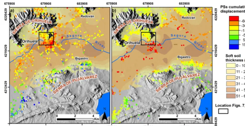
Figure 4. Cumulative displacement (mm) along the LOS superimposed to soft soil thickness for both processed periods: (a) 1995–2005 and (b) 2004–2008.
values from the subsidence activity raster maps, and rep-resents the subsidence influence area of the building where damages can be induced. From the selected cumulative dis-placement values, both the maximum differential settlement and the maximum angular distortion along the LOS are com-puted for each building (Fig. 3) and compared with the max-imum allowable values shown in Table 1.
4 Data analysis
In this section the above mentioned methodology is applied to the city of Orihuela, where SAR images covering two dif-ferent periods from July 1995 to December 2005 and from January 2004 to December 2008 have been processed using the SPN algorithm. First of all, the resulting PSI data for both processed periods are described. Then, following the first two stages of the methodology, the results obtained in the city of Orihuela for both periods are presented.
4.1 PSI data
PSI displacement maps were retrieved from the SPN processing of 110 C-band SLC SAR images from de-scending orbits acquired by the European Space Agency (ESA) ERS-1/2 and Envisat ASAR satellites covering two different periods: July 1995–December 2005 and Jan-uary 2004–December 2008 (Table 2). A similar crop of about 20 km×8 km was selected from the 100 km×100 km SAR images, corresponding to the westernmost sector of the Vega Baja of the Segura River. Interferograms were generated from pairs of SAR images with a perpendicular spatial base-line smaller than 800 m, a temporal basebase-line shorter than 6 and 3 years for the 1995–2005 and 2004–2008 periods,
re-spectively, and a relative Doppler centroid difference below 400 Hz. The digital elevation model (DEM) of the Shuttle Radar Topography Mission (SRTM) has been used. The PS selection for the estimation of displacements was based on a combination of several quality parameters including low-amplitude standard deviation and high model coherence.
Even though the reference points used for both periods are not strictly the same, they were both located in nearby stable areas of the city of Murcia, 20 km west of the city of Orihuela. Considering the whole data set for both pe-riods, the average displacement rate of the PSs included within the stable lithologies (i.e. the mountain ranges) is be-low 2 mm year−1, which is the common stability threshold adopted in the scientific literature for C-band satellite sen-sors. Moreover, the validation experiments, performed for these SPN data sets with the extensometric network in the city of Murcia (Herrera et al., 2009a, b; Tomás et al., 2011), provided a similar cumulative error (±5 mm) for both peri-ods analysed. Thus, even though the reference point is differ-ent for each period, both data sets define the same unstable areas with the same error.
Table 2. Main characteristics of the processed data stacks of the westernmost sector of Vega Baja of the Segura River:λ, wavelength;θ, look angle; Desc, descending.
Data Stack λ Orbit θ(◦) Repeat Ground Time Number Processing PS density Georeference (cm) cycle range interval of scene technique (PS km−2) accuracy (m)
(days) resolution (m)
ERS1/2 5.6 Desc 23 35 20 21/07/1995– 84 SPN 117 5
22/10/2005
ERS2 Envisat 31/01/2004– 50 50 3
20/12/2008
Table 3. Descriptive statistical measurements for both periods.
No. of PS Minimum Maximum Cumulated Displacement Standard Skewness
PS density (mm) (mm) displacements mean deviation
(PS km−2) mean (mm) (mm year−1) (mm)
1995–2005 5730 20.46 −118.88 66.78 −24.91 −2.45 21.14 −0.07
2004–2008 4922 17.58 −109.30 12.35 −20.76 −4.28 13.23 −1.85
Figure 5. PS classification according to normal distributions (first
and second components) and geological criteria for both studied pe-riods: (a) 1995–2005 and (a) 2004–2008.
the distribution of sample data) reveals that the period 2004– 2008 has a greater population of subsidence PS than the pe-riod 1995–2005. Hence, it can be concluded that the subsi-dence phenomenon is more intense in the period 2004–2008.
4.2 Spatial analysis
Once the preliminary statistical analyses were completed, the relationship between the geothematic layers and the cumula-tive displacement was studied. Tomás et al. (2010) pointed out that the geology and the thickness of alluvial soft sedi-ments were two important subsidence conditioning factors.
Table 4. Parameters of the variogram models for each normalized PS data group.
Period Geology Model Nugget Partial Effective Effective range sill range 60◦ 150◦
1995– Soft soils Exponential 0.22 0.76 3240 1860
2005
Geotechnical Exponential 0.15 0.43 1550 1300
sustratum
2004– Soft soils Spherical 0.16 1.05 4410 3150
2008
Geotechnical Spherical 0.40 0.50 4620 3920
sustratum
Figure 6. Experimental variograms with the fitted theoretical model
in 60 and 150◦directions (angles are counted from the north, in-creasing clockwise).
from the component analysis. The first component encloses stable PS on the stable rock outcrops, while the second ponent includes active PS on the younger and more com-pressible alluvial sediments. Consequently, through this anal-ysis it is demonstrated that the geology is a subsidence con-ditioning factor. Therefore, to perform PS data interpolations two different PS populations should be distinguished in each period: one in the stable sediments and another in the more deformable soft sediments.
The second conditioning factor pointed out by Tomás et al. (2010) was the thickness of alluvial soft sediments. Fig. 4 qualitatively shows a spatial correlation between soft soil thickness and cumulative ground displacements, in agree-ment with Tomás et al. (2010) stateagree-ments. Consequently, if a high linear correlation exists between the soft soil thickness and the ground displacements, the thickness could be used as a secondary variable to obtain a more accurate ground displacement interpolation. To evaluate if the soft soil thick-ness could be included as a secondary variable the Pearson correlation coefficient (McCullagh and Nelder, 1989) was calculated between the displacements and the thickness of soft soils. For this purpose the elaborated soft soil thick-ness map described in Sect. 2 was used. Note that the PSs not included within this map were not considered. The Pear-son correlation coefficient is−0.22 and −0.52 for periods 1995–2005 and 2004–2008, respectively (Appendix A). Us-ing Kaiser’s (1974) scale, the values obtained indicate that our variables have a poor linear correlation and/or other vari-ables might also be involved. Therefore, the thickness of the soft soils cannot be considered as an additional source of information for improving the displacement data interpola-tion. The observed lack of high linear correlation can be ex-plained considering that the ground displacements are the re-sult of the combined and superposed effect of piezometric level changes and the soil thickness deformability that do not follow a linear relationship.
4.3 Variogram analysis
this fact reinforces the idea that geology is a conditioning factor of subsidence.
The experimental and fitted variogram models obtained for the four PS populations previously defined are shown in Fig. 6 and described in Table 4. Experimental variograms for the 1995–2005 period present higher fluctuations around the sill than the ones computed for the 2004–2008 period. This behaviour can be attributed to the fact that during the pe-riod 1995–2005 the groundwater level was under a recuper-ation phase. Hence, measured subsidence rates are low and sparsely distributed and correspond to the residual consoli-dation of the 1992–1995 drought period. During the 2004– 2008 drought period there was an intensive exploitation of the aquifer in the vicinity of the city of Orihuela, which in-duced a regional subsidence over the area. This process ex-plains the lower spatial variability of PS displacement values, which corresponds to a lower slope of the variogram models near the origin during this period. Consequently, the analy-ses of the variogram models confirm a different subsidence spatial variability for each period, which corresponds to dif-ferent phases (piezometric level recuperation and fall) of the subsidence phenomena.
5 Results and discussion
In this section, following the last two stages of the method-ology presented in Sect. 3, the regional and local subsidence activity maps are generated and discussed for both analysed periods in the city of Orihuela. First all, the different per-centile maps are analysed. Then, the SLS for 27 historical buildings are calculated and evaluated with the reported ages inventory. Finally a comparison is made between a dam-age study and the results obtained for the Santas Justa and Rufina Church.
5.1 Regional subsidence activity maps
The parameters of the four fitted models (Table 4) are in-troduced in the SGeMS software to generate 100 equally likely realizations of subsidence by the SGS method. As the ground resolution of ERS1/2 and Envisat images is 20 m, the pixel size of the resulting surfaces has been set to 20 m. Subsidence activity maps are obtained from the SGS results. The mean of these simulations represents the expected sub-sidence value, which should be very similar to the result of the kriging interpolation (Figs. 7a, 8a). The spatial variabil-ity of the subsidence is evaluated calculating the variance for the 100 simulations performed (Figs. 7b, 8b). The confidence level for subsidence-interpolated values is established calcu-lating the percentiles from the 100 simulations. In our test site, 68th and 95th percentile maps are analysed for both pe-riods (Figs. 7c, d, 8c, d). These maps display the threshold subsidence value for which there is a probability of 68 % and 95 %, respectively, that the true subsidence is greater or equal
Figure 7. Sequential Gaussian conditional simulation results for the
1995–2005 period: (a) mean; (b) variance; (c) 68th percentile; (d) 95th percentile; and (e) location of historic buildings listed in Ta-ble 5.
to that threshold. Note that greater subsidence means a more negative value. Visually, during the period 1995–2005, the 68th and 95th percentile maps are the same, being their av-erage cumulated subsidence −17 mm. Note that the mean, which represents a 50 % confidence level, exhibits an aver-age cumulated displacement of−36 mm that is closer to the average of the PS data set (−47 mm). This fact suggests that the mean is the best estimator to elaborate subsidence activity maps in this period.
Concerning the period 2004–2008, 68th and 95th per-centiles differ substantially from each other, visually and nu-merically, with an average cumulated subsidence of−47 and
Figure 8. Sequential Gaussian conditional simulation results for the
2004–2008 period: (a) mean; (b) variance, (c) 68th percentile; (d) 95th percentile; and (e) location of historic buildings listed in Ta-ble 5.
level, and the mean for the period 1995–2005 that provides a 50 % confidence level on the interpolation.
Analysing the subsidence activity maps generated with the highest confidence level (Figs. 7a, 8c), a lower and a more lo-calized subsidence is shown in the period 1995–2005 than in the period 2004–2008, when a greater and more extended subsidence occurred. This observation is explained by the higher spatial variability (Sect. 4.3) estimated during the first period (variance between 0 and 473.07 mm2)than during the second one (variance between 0 and 387.83 mm2). Overall, the geostatistical analysis agrees with the fact that during the period 2004–2008 there was a widespread subsidence due to water withdrawal, whereas for period 1995–2005 a more heterogeneous subsidence was due to the groundwater level recuperation.
5.2 Local subsidence activity maps
The purpose at this stage is to identify those buildings sus-ceptible to suffer damage induced by subsidence based on subsidence activity maps. Following the SLS assessment methodology proposed in Sect. 3, maximum differential set-tlements and maximum angular distortions along the LOS are calculated for the 27 historical buildings of the city of Orihuela and compared with allowable values. The buffer area used in this case study is 14 m as the pixel size of the subsidence activity maps is 20 m. Note that for this resolu-tion only five pixels are considered for the SLS calcularesolu-tion of two buildings (22 and 23 in Table 5) due to their small area. In both cases, predictions might not be accurate enough and a higher resolution would be required. The results calculated for the remaining buildings indicate if the adopted SLS crite-ria exceed or do not exceed the values shown in Table 1; they represent the local subsidence activity map (Fig. 9). In these maps it is observed that the direction of both the maximum angular distortion (Fig. 9c, d) and the maximum differential settlement (Fig. 9a, b) are mainly radial to the Mesozoic re-liefs dipping towards the thickest compressible sediments.
According to SLS results (Table 5), the expected dam-age in the period 1995–2005 affects almost twice the num-ber of buildings than in the period 2004–2008. This is due to the more heterogeneous and variable spatial distribution of the 1995–2005 period displacements, which favours the existence of greater differential settlements and angular dis-tortion. Unfortunately, the lower confidence degree (50 %) obtained in the 1995–2005 period’s subsidence activity map could bias the calculation of the maximum differential set-tlement and the maximum angular distortion along the LOS (δs max-LOS,βmax-LOS). However, the greater confidence de-gree (68 %) and the lower variance obtained for the 2004– 2008 period’s subsidence activity map provides a more reli-able calculation of the service-limite state varireli-ables.
Table 5. Note that angular distortions (βmax-LOS) and (δs max-LOS) values provided by InSAR for both periods have been classified using
the font format set in Table 1 (bold for negligible, underlined for medium and italic for high). NA: not available; R: Renaissance; G: Gothic; B: Baroque; N: neoclassical; U: unknown. (∗) Total or partial underpinned foundation.
Id (Figs. 7, 8)
Name of the building
Century Style Area (m2) Period 1995–2005 Period 2004–2008 Structural damage, general de-scription (performed between 2011 and 2013)
Year of repair and/or stabilization works
Reference
δs-LOS βmax-LOS δs-LOS βmax-LOS mm (Mean) (Mean) mm (P68) (P68)
1 Santa Iglesia Catedral del Salvador
14th G, R 2473.53 15.62 4.43×10⁻⁴ 6.32 1.77×10⁻⁴ Cracks (up to 2 cm width) in
in-ternal and exin-ternal walls, in the ceiling and in a cupola. There are uncracked plaster markers. The S and W façades exhibit apparently ancient tilts.
1990, 2002∗ Lara (2003) and field work
2 Colegio
Diocesano Santo Domingo
16th R 9962.95 27.51 9.43×10⁻⁴ 9.42 1.89×10⁻⁴ Cracks in internal and
exter-nal walls of the cloister (up to 6 cm in the refectory). Most of the cylindrical vaults from the corridors also present millimet-ric to submillimetmillimet-ric fissures. The annexed church presents a clearly ancient tilt. Some plas-ter markers placed in the clois-ter in 2000 are uncracked.
2002 (only the Comunión Chapel was repaired)∗ Lara (2003), Maciá (2005) and field work
3 Iglesia Parroquial de Santiago Apostol
15th G 1881.50 4.96 1.94×10⁻⁴ 16.35 7.63×10⁻⁴ Good overall condition. Most of the damages are located in the SW corner and consist of cracks and fissures affecting the walls and the ceiling.
1993, 2002∗ Lara (2003) and field work
4 Santuario de Nuestra Señora de Monserrate
17th B 2031.75 26.97 7.54×10⁻⁴ 14.43 4.34×10⁻⁴ Cracks on the bell towers, the internal and external walls, in the vaults and cupolas.
None Field work
5 Iglesia Parroquial de San Antón
18th B 263.88 5.64 2.27×10⁻⁴ 0.63 3.17×10⁻⁵ NA NA
6 Santas Justa and Rufina Church
14th G 1880.13 15.18 3.99×10⁻⁴ 19.16 6.41×10⁻⁴ Millimetre to centimetre cracks on the internal and external walls of the main building. The eastern wall presents an ancient tilt. The cupola from the Co-munión Chapel presents a cen-timetric crack.
1970, 2002, 2010∗
Lara (2003) and Tomás et al. (2012)
7 Ermita del Santo Sepulcro
17th B 348.74 9.65 4.82×10⁻⁴ 1.60 8.00×10⁻⁵ NA NA
8 Seminario Diocesano de San Miguel
18th B 6933.81 9.99 3.53×10⁻⁴ 5.50 2.42×10⁻⁴ NA NA
9 Iglesia y convento del Carmen
18th B 1230.62 19.41 4.98×10⁻⁴ 4.08 1.49×10⁻⁴ Cracks on the external walls from the main building. The number of cracks (with a submillimetre width) increases in the internal face of the walls. Most of the cylindrical vaults present submillimetric– millimetric fissures. There are some uncracked plaster markers placed in 2007.
1986, 2004 Field work
10 Real Monasterio de las Religiosas Salesas
18th N 2895.02 20.10 5.67×10⁻⁴ 6.78 2.08×10⁻⁴ 45◦cracks (with a subcentimet-ric width) on the façades from the main building coinciding with the window corners. Inside the building, Louis (2005) de-scribed important irregularities caused by ground settlements in the pavement of the convent which were repaired in 2008.
2008 Louis (2005) and field work
11 Monasterio de San Juan Bautista de la Penitencia
15th B 2840.28 14.72 4.43×10⁻⁴ 6.10 1.98×10⁻⁴ NA NA
12 Monasterio de la Santísima Trinidad
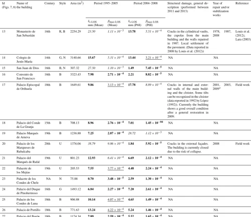
Table 6. Continued.
Id (Figs. 7, 8)
Name of the building
Century Style Area (m2) Period 1995–2005 Period 2004–2008 Structural damage, general de-scription (performed between 2011 and 2013)
Year of repair and/or stabilization works
Reference
δs-LOS βmax-LOS δs-LOS βmax-LOS mm (Mean) (Mean) mm (P68) (P68)
13 Monasterio de San Sebastián
16th R, B 2254.29 23.50 1.11×10⁻³ 13.78 5.51×10⁻⁴ Cracks in the cylindrical vaults, the cupolas from the main building and the walls repaired in 1987. Local settlement of the pavement. (Data reported in 2008 by Louis et al. (2012))
1978, 1987, 2008
Louis et al. (2012); Lara (2003)
14 Colegio de Jesús-María
14th G, N 3140.66 15.67 5.31×10⁻⁴ 13.44 3.21×10⁻⁴ NA NA
15 San Juan de Dios 16th B, N 307.32 27.50 1.10×10⁻³ 1.49 7.45×10⁻⁵ NA NA
16 Convento de San Francisco
16th B 3323.43 7.98 2.71×10⁻⁴ 2.21 8.82×10⁻⁵ NA NA
17 Palacio Episcopal de Orihuela
18th B 1649.61 9.86 3.13×10⁻⁴ 17.78 8.89×10⁻⁴ Cracks in internal and exter-nal walls of the main build-ing and the cloister. Some tilts can be recognized in the cloister (data reported in 1992 by López (1992)). Currently the building shows a good overall condition after a general restoration in 2009.
2001, 2003, 2009∗
Field work
18 Palacio del Conde de La Granja
15th B 708.13 8.96 2.76×10⁻⁴ 7.01 1.45×10−04 NA NA
19 Palacio Marqués de Arneva
19th B 1236.88 7.25 2.87×10⁻⁴ 28.72 1.12×10⁻³ NA NA
20 Palacio de los Marqueses de Rubalcaba
20th U 1376.06 38.79 9.86×10⁻⁴ 1.84 5.92×10⁻⁵ Cracks in the external façades.
The building is currently closed due to the risk of collapse.
2008 Field work
21 Palacio del Marqués de Rafal
19th U 801.23 12.93 6.41×10⁻⁴ 6.69 2.12×10⁻⁴ NA NA
22 Palacete de los Mejías
19th U 205.53 7.55 3.77×10⁻⁴ 4.48 2.24×10⁻⁴ NA NA
23 Palacete de los Condes de Chele
NA N 75.88 0.70 3.48×10⁻⁵ 2.59 1.30×10⁻⁴ NA NA
24 Palacio del Duque de Pinohermoso
16th G 1493.12 6.84 2.27×10⁻⁴ 7.20 2.61×10⁻⁴ NA NA
25 Palacio de los Condes de Luna
18th B 906.88 10.14 4.07×10⁻⁴ 4.65 1.49×10⁻⁴ NA NA
26 Palacio de Portillo 18th B 771.63 13.24 4.22×10⁻⁴ 5.24 1.46×10⁻⁴ NA NA
27 Palacio del Barón de la Linde
18th B 1174.34 7.89 2.59×10⁻⁴ 5.52 1.65×10⁻⁴ NA NA
expected after the repair actions. Additionally, we have to consider that damages are repaired in different phases that can extend over years, acting on different parts of the build-ing (e.g. in the Santas Justa and Rufina Church the foundation was only partially underpinned and part of the church is still supported by the old foundation).
Considering the heterogeneity of the available informa-tion and the previously meninforma-tioned constrains that can dis-tort the interpretation of the results, reported damages (Ta-ble 5) have only been used for a qualitative evaluation of local subsidence activity maps. Nevertheless, 100 % of the build-ings (over 10) where damages have been reported exhibit “medium” to “high” levels of expected damages according to SLS calculations. Note that during the 1995–2005 period 90 % of the buildings (over 10) exceeded the allowable SLS
while for the 2004–2008 period this rate dropped to 50 % of the buildings (over 10). In this context, damages observed on several buildings (2, 3, 4, 6, 9, 10, 13 and 20) can be at-tributed to cumulated subsidence during both periods, since no restoration activities were performed. For these buildings subsidence activity maps show a good agreement with the observed damage since the SLS threshold values were ex-ceeded in at least one of the two periods.
Figure 9. Local subsidence activity maps for both periods studied. Notice that the interpolation surfaces used are the mean and the 68th
percentile for 1995–2005 and the 2004–2008 periods, respectively.
even if a good overall condition was recognized during re-cent field work. This mismatch is explained by the build-ing’s restoration in 2009. Additionally López (1992) recog-nized numerous damages that could be related to the ex-pected “medium” and “high” levels of damage calculated for the 1995–2005 and 2004–2008 periods, respectively.
Analyzing those buildings where no information about their SLS state could be gathered, buildings 12 and 15 (Ta-ble 5) show in both periods, an expected “high” or “medium” level of damage and should be considered as priority targets
Figure 10. Location of the structural damage and restoration and
reinforcement actions performed on the Santas Justa and Rufina Church (modified from Tomás et al., 2012).
5.3 Analysis of the Santas Justa and Rufina Church
A more detailed analysis of the local subsidence activity map is carried out in the Santas Justa and Rufina Church, where a forensic analysis is available. The Santas Justa and Rufina Church is located on the north bank of the Segura River in the centre of the city of Orihuela (Fig. 7 and 8). It was de-clared a Spanish National Monument in 1971. During the last 20 years damages induced by regional subsidence have af-fected the structural elements of this church (Fig. 10). Tomás et al. (2012) performed a detailed analysis of the damage suf-fered by the building, summarized here. In the 1970 s the principal chapel suffered an important tilt (Fig. 10). In the 1990 s, important settlements affected the San José Chapel and the foundation was reinforced in 2002 with micropiles. In the first decade of the present century, displacements af-fected the whole north zone of the church and the principal chapel area. Multiple cracks where identified in the north, west, and east walls, affecting as well La Comunión Cupola (Fig. 10a), the sacristy and the antesacristy (Fig. 10c). Sev-eral plaster markers were placed in the cracks in 2006 and controlled in 2008 (Fig. 10b). Figure 10 shows that multiple cracks grew during this period as a consequence of the sink-ing of the foundation walls caused by ground subsidence.
Subsidence activity maps, maximum differential settle-ment and maximum angular distortion along the LOS, of the Santas Justa and Rufina Church are shown in Fig. 11. The average cumulated displacements are−39.2 and−31.9 mm
for the 1995–2005 and 2004–2008 periods, respectively, but a greater variance is appreciated for the first period. The max-imum angular distortion shows medium (1995–2005) to high (2004–2008) values. Note that during the first period, the maximum angular distortion is located NE of the church, mainly affecting the main chapel. However, it is observed that during the second period the maximum angular distor-tion is located SW of La Comunión Chapel. The orientadistor-tion of the two vectors representing the maximum angular dis-tortion is E–W, which is in agreement with the location of reported damages (Fig. 10). Concerning the maximum differ-ential settlement, the vector direction (NE–SW) is the same for both periods. This would indicate that the church would have tilted towards the SW and as a consequence the direc-tions of cracks (normal to tension stresses) are expected to be oriented from NW to SE, coinciding with the reported damages (Fig. 10). Even if the 23.01 mm threshold has not been exceeded in each period, and taking into account that the direction of both vectors is similar, the combination of them yields a 34 mm maximum differential settlement. One can say that the reported damages match, spatially and tem-porally, with the calculated SLS.
6 Conclusions
This work proposes a novel method to produce subsidence activity maps based on the geostatistical analysis of persis-tent scatterer interferometry (PSI) displacement data. These maps permit us to identify widespread subsiding areas and buildings where damages could be produced, providing a useful tool for the planning and management activities of the local authorities. However, the derived results cannot be ex-ploited in an isolated way. They need to be combined with in situ field data to confirm the potential levels of damage. The methodology has been tested in 27 historical buildings of the city of Orihuela (SE Spain), which have been damaged in past decades due to subsidence triggered by groundwater overexploitation.
The spatial analysis and directional variograms revealed that geology is a subsidence conditioning factor that should be taken into account when performing a geostatistical anal-ysis. The variogram-fitted models differ for each period, confirming a different spatio-temporal subsidence behaviour, which is explained by groundwater level changes during droughts. The conditional sequential Gaussian simulation (SGS) provided realistic subsidence estimations including the evaluation of its confidence degree level and its spatial variability.
Figure 11. Mean (1995–2005), 68th percentile (2004–2008) and
variance for both studied periods in the vicinity of the Santas Justa and Rufina Church.
parameters: the differential settlement and the angular distor-tion. In 27 historical buildings of the city of Orihuela, SLS results have been compared with reported damages and field checks available for 10 buildings, showing a 100 % success rate. Additionally, SLS allowed distinguishing two groups of potentially damaged buildings, enabling us to establish an inspection priority in agreement with the expected level of damage.
Appendix A
Appendix B:
Table B1. List of processed SAR images.
Date Sensor Date Sensor Date Sensor Date SENSOR
21/07/1995 ERS1 18/12/1999 ERS2 18/10/2003 Envisat 17/09/2005 Envisat 26/08/1995 ERS2 22/01/2000 ERS2 18/10/2003 ERS2 22/10/2005 ERS2 30/09/1995 ERS2 26/02/2000 ERS2 22/11/2003 ERS2 26/11/2005 Envisat 04/11/1995 ERS2 01/04/2000 ERS2 27/12/2003 ERS2 26/11/2005 ERS2 26/04/1996 ERS1 06/05/2000 ERS2 31/01/2004 ERS2 31/12/2005 Envisat 19/10/1996 ERS2 15/07/2000 ERS2 31/01/2004 Envisat 31/12/2005 ERS2 23/11/1996 ERS2 19/08/2000 ERS2 06/03/2004 Envisat 11/03/2006 ERS2 12/04/1997 ERS2 23/09/2000 ERS2 10/04/2004 ERS2 15/04/2006 Envisat 17/05/1997 ERS2 28/10/2000 ERS2 15/05/2004 Envisat 20/05/2006 ERS2 26/07/1997 ERS2 02/12/2000 ERS2 15/05/2004 ERS2 24/06/2006 ERS2 30/08/1997 ERS2 06/01/2001 ERS2 19/06/2004 ERS2 02/09/2006 Envisat 04/10/1997 ERS2 04/08/2001 ERS2 19/06/2004 Envisat 07/10/2006 Envisat 08/11/1997 ERS2 08/09/2001 ERS2 24/07/2004 ERS2 11/11/2006 ERS2 17/01/1998 ERS2 13/10/2001 ERS2 28/08/2004 ERS2 31/03/2007 Envisat 28/03/1998 ERS2 17/11/2001 ERS2 02/10/2004 ERS2 31/03/2007 Envisat 11/07/1998 ERS2 22/12/2001 ERS2 06/11/2004 ERS2 05/05/2007 Envisat 19/09/1998 ERS2 02/03/2002 ERS2 11/12/2004 ERS2 18/08/2007 Envisat 28/11/1998 ERS2 06/04/2002 ERS2 11/12/2004 Envisat 05/01/2008 Envisat 13/03/1999 ERS2 11/05/2002 ERS2 15/01/2005 Envisat 09/02/2008 Envisat 17/04/1999 ERS2 15/06/2002 ERS2 19/02/2005 Envisat 15/03/2008 Envisat 22/05/1999 ERS2 20/07/2002 ERS2 19/02/2005 ERS2 24/05/2008 Envisat 30/07/1999 ERS1 24/08/2002 ERS2 26/03/2005 Envisat 28/06/2008 Envisat 31/07/1999 ERS2 28/09/2002 ERS2 26/03/2005 ERS3 28/06/2008 Envisat 03/09/1999 ERS1 02/11/2002 ERS2 30/04/2005 Envisat 02/08/2008 Envisat 04/09/1999 ERS2 11/01/2003 ERS2 04/06/2005 ERS2 06/09/2008 Envisat 09/10/1999 ERS2 22/03/2003 Envisat 09/07/2005 ERS2 11/10/2008 Envisat 13/11/1999 ERS2 26/04/2003 ERS2 13/08/2005 ERS2 15/11/2008 Envisat
Acknowledgements. The authors would like to honour the memory of Enrique Chacón Oreja, professor at the School of Mines, who sadly passed away before the publication of this article. His ideas were the inspiration of this work.
The European Space Agency (ESA) Terrafirma project has funded all the SAR data processing with the SPN technique. Additionally, this work has been partially financed by DORIS project (Ground deformation risk scenarios: an advanced as-sessment service) funded by the EC-GMES-FP7 initiative (grant agreement no. 242212), and the Spanish Geological and Mining Institute (IGME). This work has been also supported by the Spanish Ministry of Science and Research (MICINN) under project TEC2011-28201-C02-02 and EU FEDER.
Edited by: F. Guzzetti
Reviewed by: three anonymous referees
References
Arangio, S., Calò, F., Di Mauro, M., Bonano, M., Marsella, M., and Manunta, M.: An application of the SBAS-DInSAR technique for the Assessment of structural damage in the city of Rome, in: Structure and Infrastructure Engineering: Maintenance, Management, Life-Cy. Design Perform., 1–15, doi:10.1080/15732479.2013.833949, 2013.
Armstrong, M.: Problems with universal kriging, J. Internat. Ass. Mathemat. Geol., 16, 101–108, 1984.
Arnaud, A., Adam, N., Hanssen, R., Inglada, J., Duro, J., Closa, J., and Eineder, M.: ASAR ERS interferometric phase continu-ity, Geoscience and Remote Sensing Symposium, 2003, IGARSS ’03, Proceedings, 2003 IEEE International, 21–25 July 2003, 2, 1133–1135, 2003.
Benaglia, T., Chauveau, D., Hunter, D. R., and Young, D.: “mix-tools”: an R package for analyzing finite mixture models, J. Statist. Software, 32, 1–29, 2009.
Berardino, P., Fornaro, G., Lanari, R., and Sansosti, E.: A new algo-rithm for surface deformation monitoring based on small base-line differential SAR interferograms, IEEE Trans. Geosci. Re-mote Sens., 40, 2375–2383, 2002.
Bjerrum, L.: Allowable settlement of structures. Proceedings of the 3rd European Conference on Soil Mechanics and Foundation En-gineering, Wiesbaden, Germany, 2, 135–137, 1963.
Boscardin, M. D. and Cording J. C.: Building response to excavation-induced settlement, J. Geotechn. Engin., ASCE, 115, 1–21, 1989.
Bru, G., Herrera, G., Tomás, R., Duro, J., De la Vega, R., and Mulas, J.: Control of deformation of buildings affected by subsidence us-ing persistent scatterer interferometry, Struct. Infrastructure En-gin., 9, 188–200, 2010.
Burland, J. B. and Wroth, C. P.: Settlement of buildings and asso-ciated damage. Proceedings of the Conference on Settlement of Structures, Cambridge, UK, Pentech Press, London, UK, 611– 654, 1974.
Burland, J. B., Broms, B. B., and de Mello, V. F.: Behaviour of foundations and structures, S.O.A. Report. IX ICSMFE, Tokyo, 2, 495–546, 1977.
Burrough, P. A and McDonnell, R.: Principles of Geographical Information Systems (vol. 333). Oxford University Press, New York, 1998.
Cascini, L., Ferlisi, S., Peduto, D., Fornaro G., and Manunta M.: Analysis of a subsidence phenomenon via DInSAR data and geotechnical criteria, Italian Geotechn. J., 41, 50–67, 2007. Cigna, F., Del Ventisette, C., Liguori, V., and Casagli, N.: Advanced
radar-interpretation of InSAR time series for mapping and char-acterization of geological processes, Nat. Hazards Earth Syst. Sci., 11, 865–881, doi:10.5194/nhess-11-865-2011, 2011. Cigna, F., Del Ventisette, C., Gigli, G., Menna, F., Agili, F., Liguori,
V., and Casagli, N.: Ground instability in the old town of Agri-gento (Italy) depicted by on-site investigations and Persistent Scatterers data, Nat. Hazards Earth Syst. Sci., 12, 3589–3603, doi:10.5194/nhess-12-3589-2012, 2012.
CTE: Código Técnico de la Edificación, SE-C Seguridad structural de cimientos, 160 pp., 2006 (in Spanish).
de Boer, A., Egeler, C. G., Kampschuur, W., Montenat, C., Rondeel, H. E., Simon, O. J., and van Winkoop, A. A.: Mapa Geológico de España, 1:50 000, IGME, Hoja 913, Orihuela, 1982. Delgado, J., López Casado, C., Estévez, A., Giner, J., Cuenca, A.,
and Molina, S.: Mapping soft soils in the Segura river valley (SE Spain): a case study of microtremors as an exploration tool, J. Appl. Geophys., 45, 19–32, 2000.
Duro, J., Inglada, J., Closa, J., Adam, N., and Arnaud, A.: High resolution differential interferometry using time series of ERS and ENVISAT SAR data, in: FRINGE 2003,Frascati, Italy, 1–5 December 2005.
EN: 2002 Eurocode – Basis of Structural Design, CEN, 29 Novem-ber 2001, 1990.
Ferretti, A., Prati, C., and Rocca, F.: Permanent scatterers in SAR interferometry, IEEE Transact. Geosci. Remote Sens., 39, 8–20, 2001.
Ferretti, A., Fumagalli, A., Novali, F., Prati, C., Rocca, F., and Rucci, A.: new algorithm for processing interferometric data-stacks, SqueeSAR, IEEE Transact. Geosci. Remote Sens., 49, 3460–70, 2011.
Galloway, D. and Hoffmann, J.: The application of satellite differ-ential SAR interferometry-derived ground displacements in hy-drogeology, Hydrogeol, J., 15, 133–154, 2007.
Galloway, D. and Burbey, T.: Review: regional land subsidence ac-companying groundwater extraction, Hydrogeol. J., 19, 1459– 1486, 2011.
Galloway, D. L., Jones, D. R., and Ingebritsen, S. E.: Land Subsi-dence in the United States US, Geological Survey Circular US, Geological Survey, Reston, Virginia, p. 177, 1999.
Gómez-Hernández, J. J. and Journel, A. G.: Joint Sequential Sim-ulation of MultiGaussian Fields. InGeostatistics Tróia ’92, A. Soares (editor), Kluwer Academic Publishers, 1, 85–94, 1993. Goovaerts, P.: Geostatistics for Natural Resources Evaluation.
Ox-ford University Press, New York, 1997.
Heleno, S. I. N., Oliveira, L. G. S., Henriques, M. J., Falcão, A. P., Lima, J. N. P., Cooksley, G., Ferretti, A., Fonseca, A. M., Lobo-Ferreira, J. P., and Fonseca, J. F. B. D.: Persistent scatterers in-terferometry detects and measures ground subsidence in Lisbon, Remote Sens. Environ., 115, 2152–2167, 2011.
Herrera, G., Tomás, R., López–Sánchez, J. M., Delgado, J., Vi-cente, F., Mulas, J., Cooksley, G., Sánchez, M., Duro, J., Ar-naud, A., Blanco, P., Duque, S., Mallorquí, J. J., Vega–Panizo, R., and Monserrat, O.: Validation and comparison of Advanced Dif-ferential Interferometry Techniques: Murcia metropolitan area case study, ISPRS J. Photogramm. Remote Sens., 64, 501–512, 2009b.
Herrera, G., Tomás, R., Monells, D., Centolanza, G., Mallorquí, J. J., Vicente, F., Navarro, V. D., Lopez-Sanchez, J. M., Sanabria, M., Cano, M., and Mulas, J.: Analysis of subsidence using TerraSAR-X data: Murcia case study, Engin. Geol., 116, 284– 295, 2010.
Hung, W., Hwang, C., Chen, Y., Chang, C., Yen, J., Hooper, A., and Yang, J.: Surface deformation from persistent scatterers SAR in-terferometry and fusion with leveling data: A case study over the Choushui River Alluvial Fan, Taiwan, Remote Sens. Environ., 115, 957–967, 2011.
IGME: Calidad de Las Aguas Subterrá neas en la Cuenca Baja del Segura y Costeras de Alicante. Instituto Geológico y Minero, Madrid, Technical Report, 77 pp., 1986.
Isaaks, E. H and Srivastava, R. M.: Applied Geostatistics, Oxford University Press, New York, 1989.
Journel, A. G. and Huijbregts, C. J.: Mining Geostatistics (vol. 859), London Academic press, London, 1978.
Kaiser, H.: An index of factorial simplicity, Psychometrika, 39, 31– 36, 1974.
Karila, K., Karjalainen, M., and Hyyppä, J.: Urban Land Subsidence Studies in Finland Using Synthetic Aperture Radar Images and Coherent Targets, Photogramm. J. Finland, 19, 43–53, 2005. Lara, S.: Las arquitecturas de Semblantes de la vida, Ed. Servicio de
Publicaciones de la UPV, Valencia, España, ISBN 84-607-9540-3, 164 pp., 2003.
López, S.: Restauración del Palacio Episcopal de Orihuela, Docu-mento 1 Memoria y anexos, Tomo II, Anexos arquitectura, Fase 1, Capítulo 3: Investigación patológica, Technical Report, Inedit, 259–262, 1992.
Louis, M.: Toma de datos y proyecto restauración Iglesia las Sale-sas (Orihuela), Septiembre 2005, Technical Report, unpublished, 2005.
Louis, M., Spairani, Y., Huesca, J. A., and Prado, R.: La restau-ración de la iglesia de San Sebastián, Orihuela (Alicante), in: XI Congreso Internacional de Rehabilitación del Patrimonio Arqui-tectónico y Edificación , edited by: Servicio de Publicaciones de la Fundación Centro Internacional para la Conservación del Pat-rimonio (CICOP), Cascais, Portugal: Servicio de Publicaciones de la Fundación Centro Internacional para la Conservación del Patrimonio (CICOP), 202–210, 2012.
Maciá, J. A.: Estudio diagnóstico y propuesta de intervenciones en el colegio Diocesano Santo Domingo, Technical Report, unpub-lished, 2005.
Martínez, M., Mulas, J., Herrera, G., and Aragón, R.: Efectos de una subsidencia moderada por extracción de agua subterránea en Murcia, España, Proc. XXXIII Congress of IAH-ALHSUD, Za-catecas, Mexico, Conference on Groundwater Flow Understand-ing from local to regional scales, CD ROM, 2004.
Massonnet, D., Rossi, M., Carmona, C., Adragna, F., Peltzer, G., Feigl, K., and Rabaute, T.: The displacement field of the Landers earthquake mapped by radar interferometry, Nature, 364, 138– 142, 1993.
Matheron, G.: Principles of geostatistics, Econ. Geol., 58, 1246– 1266, 1963.
McCullagh, P. and Nelder, J. A.: Generalized Linear Models, Chap-man and Hall, London, 1989.
Mora, O., Mallorquí, J. J., and Broquetas, A.: Linear and nonlinear terrain deformation maps from a reduced set of interferometric SAR images, IEEE Transact. Geosci. Remote Sens., 41, 2243– 2253, 2003.
Mulas, J., Aragón, R., Martínez, M., Lambán, J., García-Arostegui, J. L., Fernández-Grillo, A. I., Hornero, J., Rodríguez, J., and Ro-dríguez, J. M.: Geotechnical and hydrological analysis of land subsidence in Murcia (Spain), Proc. 1-International Conference on Groundwater in Geological Engineering, 22–26 September, Bled, Slovenia, 50, 249–252, 2003
Namazi, E. and Mohamad, H.: Potential damage assessment in buildings undergoing tilt, Proceedings of the ICE – Geotechni-cal Engineering, 365–375, 2013.
Olea, R. A.: Fundamentals of semivariogram estimation, modeling, and usage, in: AAPG Computer Applications in Geology No. 3, edited by: Yarus, J. M., and Chambers, R. L., Chapter 4, 27-35, 1994.
Pebesma, E. J.: Multivariable geostatistics in S: the gstat package, Comput. Geosci., 30, 683–691, 2004.
Peltzer, G. and Rosen, P.: Surface Displacement of the 17 May 1993 Eureka Valley, California, Earthquake Observed by SAR Inter-ferometry, Science, 268, 1333–1336, 1995.
Poland, J. F., Yamamoto, S., and working group: Field measure-ments of deformation, in: Guidebook to studies of land subsi-dence due to ground-water withdrawal: United Nations Educa-tional, Scientific and Cultural Organization,Poland, edited by: J. F., Paris, Studies and Reports in Hydrology, 40, 17–36, 1984. Prati, C., Ferretti, A., and Perissin, D.: Recent advances on surface
ground deformation measurement by means of repeated space-borne SAR observations, J. Geodyn., 49, 161–170, 2010. R Development Core Team: A language and environment for
statis-tical computing. R Foundation for Statisstatis-tical Computing, Vienna, Austria, http://www.R-project.org., ISBN 3-900051-07-0, 2010. Raspini, F., Cigna, F., and Moretti, S.: Multi-temporal mapping of land subsidence at basin scale exploiting Persistent Scatterer In-terferometry: case study of Gioia Tauro plain (Italy), J. Maps, 8, 514–524, 2012.
Raucoules, D., Bourgine, B., De Michele, M., Le Cozannet, G., Closset, L., Bremmer, C., Veldkamp, H., Tragheim, D., Bateson, L., Crosetto, M., Agudo, M., and Engdahl, M.: Validation and Intercomparison of Persistent Scatterers Interferometry: PSIC4 project results, J. Appl. Geophys., 68, 335–347, 2009.
Remy, N., Boucher, A., and Wu, J.: Applied Geostatistics with SGeMS: A User’s Guide, UK, Cambridge University Press, 2009.
Ribeiro, Jr. P. J. and Peter, J.: Diggle geoR: a package for geostatis-tical analysis R-NEWS, 1, 15–18, 2001.
Sanabria, M. P., Guardiola-Albert, C., Tomás, R., Cooksley, C., and Herrera, G.: Geostatistical Analysis of PSI Radar Data: A Methodology to Assess Serviceable Limit State of Buildingsin Mathematics of Planet Earth, Lecture Notes in Earth System Sci-ences, 267–270, 2014.
sur-face displacement analysis, Geophys. Res. Lett., 37, L20305, doi:10.1029/2010GL044379, 2010.
Skempton, A. W. and McDonalds, D. H.: Allowable settlements of buildings, Proc. ICE, London, 5, 727–768, 1956.
Sousa, J. J. and Bastos, L.: Multi-temporal SAR interferometry re-veals acceleration of bridge sinking before collapse, Nat. Haz-ards Earth Syst, Sci., 13, 659–667, doi:10.5194/nhess-13-659-2013, 2013.
Sowter, A., Bateson, L., Strange, P., Ambrose, K., and Sya?udin, M.: DInSAR estimation of land motion using intermittent coher-ence with application to the South Derbyshire and Leicestershire coalfield, Remote Sens. Lett., 4, 979–987, 2013.
Stramondo, S., Bozzano, F., Marra, F., Wegmuller, U., Cinti, F. R., Moro, M., and Saroli, M.: Subsidence induced by urbanization in the city of Rome detected by advanced InSAR technique and geotechnical investigations, Remote Sens. Environ., 112, 3160– 3172, 2008.
Tapete, D., Fanti, R., Cecchi, R. Petrangeli, P., and Casagli, N.: Satellite radar interferometry for monitoring and early-stage warning of structural instability in archaeological sites, J. Geo-phys. Engin., 9, S10–S25, 2012.
Terzaghi, K. and Peck, R. B.: Soil Mechanics in Engineering Prac-tice, John Wiley and Sons, New York, 1948.
Tomás, R., Domenech, Mira, A., Cuenca, A., and Delgado, J.: Pre-consolidation stress in the Vega Baja and Media areas of the River Segura (SE Spain): causes and relationship with piezomet-ric level changes, Engin. Geol., 91, 135–151, 2007a.
Tomás, R., Lopez-Sanchez, J. M., Delgado, J., Vicente, F., Cuenca, A., Mallorquí, J. J., Blanco, P., and Duque, S.: DInSAR mon-itoring of land subsidence in Orihuela city, Spain: Comparison with geotechnical data, 2007 International Geoscience and Re-mote Sensing Symposium, Barcelona, 2007b.
Tomás, R., Herrera, G., Lopez-Sanchez, J. M., Vicente, F., Cuenca, A., and Mallorquí, J. J.: Study of the land subsidence in the Orihuela city (SE Spain) using PSI data: distribution, evolution and correlation with conditioning and triggering factors, Engin. Geol., 115, 105–121, 2010.
Tomás, R., Herrera, G., Cooksley, G., and Mulas, J.: Persistent Scat-terer Interferometry subsidence data exploitation using spatial tools: The Vega Media of the Segura River Basin case study, J. Hydrol., 400, 411–428, 2011.
Tomás, R., García-Barba, J., Cano, M., Sanabria, M. P., Ivorra, S., Duro, J., and Herrera, G.: Subsidence damage assessment of a gothic church using Differential Interferometry and field data, Struct. Health Monit., 11, 751–762, 2012.