University of Pennsylvania
ScholarlyCommons
Publicly Accessible Penn Dissertations
1-1-2013
Bayesian Aspects of Classification Procedures
Igar Fuki
University of Pennsylvania, [email protected]
Follow this and additional works at:http://repository.upenn.edu/edissertations Part of theStatistics and Probability Commons
This paper is posted at ScholarlyCommons.http://repository.upenn.edu/edissertations/863
Recommended Citation
Fuki, Igar, "Bayesian Aspects of Classification Procedures" (2013).Publicly Accessible Penn Dissertations. 863.
Bayesian Aspects of Classification Procedures
Abstract
We consider several statistical approaches to binary classification and multiple hypothesis testing problems. Situations in which a binary choice must be made are common in science. Usually, there is uncertainty involved in making the choice and a great number of statistical techniques have been put forth to help researchers deal with this uncertainty in separating signal from noise in reasonable ways. For example, in genetic studies, one may want to identify genes that affect a certain biological process from among a larger set of genes. In such examples, costs are attached to making incorrect choices and many choices must be made at the same time. Reasonable ways of modeling the cost structure and choosing the appropriate criteria for evaluating the performance of statistical techniques are needed. The following three chapters have proposals of some Bayesian methods for these issues.
In the first chapter, we focus on an empirical Bayes approach to a popular binary classification problem formulation. In this framework, observations are treated as independent draws from a hierarchical model with a mixture prior distribution. The mixture prior combines prior distributions for the ``noise'' and for the ``signal'' observations. In the literature, parametric assumptions are usually made about the prior distribution from which the ``signal'' observations come. We suggest a Bayes classification rule which minimizes the expectation of a flexible and easily interpretable mixture loss function which brings together constant penalties for false positive misclassifications and $L_2$ penalties for false negative misclassifications. Due in part to the form of the loss function, empirical Bayes techniques can then be used to construct the Bayes classification rule without specifying the ``signal'' part of the mixture prior distribution. The proposed classification technique builds directly on the nonparametric mixture prior approach proposed by Raykar and Zhao (2010, 2011).
Many different criteria can be used to judge the success of a classification procedure. A very useful criterion called the False Discovery Rate (FDR) was introduced by Benjamini and Hochberg in a 1995 paper. For many applications, the FDR, which is defined as the expected proportion of false positive results among the
observations declared to be ``signal'', is a reasonable criterion to target. Bayesian versions of the false
discovery rate, the so-called positive false discovery rate (pFDR) and local false discovery rate, were proposed by Storey (2002, 2003) and Efron and coauthors (2001), respectively. There is an interesting connection between the local false discovery rate and the nonparametric mixture prior approach for binary classification problems. The second part of the dissertation is focused on this link and provides a comparison of various approaches for estimating Bayesian false discovery rates.
The third chapter is an account of a connection between the celebrated Neyman-Pearson lemma and the area (AUC) under the receiver operating characteristic (ROC) curve when the observations that need to be classified come from a pair of normal distributions. Using this connection, it is possible to derive a classification rule which maximizes the AUC for binormal data.
Degree Type
Dissertation
Degree Name
Graduate Group
Statistics
First Advisor
Linda H. Zhao
Keywords
Classification procedures, empirical Bayes, False discovery rate, nonparametric mixture prior
Subject Categories
BAYESIAN ASPECTS OF
CLASSIFICATION
PROCEDURES
Igar Fuki
A DISSERTATION
in
Statistics
For the Graduate Group in Managerial Science and Applied
Economics
Presented to the Faculties of the University of Pennsylvania
in
Partial Fulfillment of the Requirements for the
Degree of Doctor of Philosophy
2013
Supervisor of Dissertation
Linda Zhao, Professor, Statistics
Graduate Group Chairperson
Eric Bradlow, K.P. Chao Professor, Marketing, Statistics and Education
Dissertation Committee
Linda Zhao, Professor of Statistics
BAYESIAN ASPECTS OF CLASSIFICATION PROCEDURES
COPYRIGHT
2013
Igar Fuki
This work is licensed under the Creative Commons
Attribution-NonCommercial-ShareAlike 3.0 License
To view a copy of this license, visit
Acknowledgement
This dissertation and all of my projects in graduate school would not have been
possible without Linda Zhao. I would like to thank her for her incredible help and
support. Professor Zhao not only set out my research path, but was a source of
strength during the most difficult times. Thank you for everything.
I would like to thank my committee members, Lawrence Brown and Fernando
Ferreira, for their help and invaluable advice with my dissertation. I would also like
to express my deepest gratitude to Marja Hoek-Smit, whose door was always open
for me.
Thank you to Todd Sinai, Warren Ewens, Murray Gerstenhaber, Carol Reich,
Keith Weigelt, Daniel Yekutieli, and W. Bruce Allen for their guidance and advice.
My thanks also to Vikas Raykar and Xu Han.
This thesis is based on several joint working papers, and I would like to thank my
senior co-authors for their contributions to the text, for their inspiration, and for
teaching me about research and scientific writing.
Thank you also to the faculty, staff, and students of the Statistics and Real Estate
departments at Wharton, and to many others at the University of Pennsylvania for
all of their help.
ABSTRACT
BAYESIAN ASPECTS OF CLASSIFICATION
PROCEDURES
Igar Fuki
Linda Zhao
We consider several statistical approaches to binary classification and multiple
hypothesis testing problems. Situations in which a binary choice must be made
are common in science. Usually, there is uncertainty involved in making the choice
and a great number of statistical techniques have been put forth to help researchers
deal with this uncertainty in separating signal from noise in reasonable ways. For
example, in genetic studies, one may want to identify genes that affect a certain
biological process from among a larger set of genes. In such examples, costs are
attached to making incorrect choices and many choices must be made at the same
time. Reasonable ways of modeling the cost structure and choosing the appropriate
criteria for evaluating the performance of statistical techniques are needed. The
following three chapters have proposals of some Bayesian methods for these issues.
In the first chapter, we focus on an empirical Bayes approach to a popular binary
classification problem formulation. In this framework, observations are treated as
The mixture prior combines prior distributions for the “noise” and for the “signal”
observations. In the literature, parametric assumptions are usually made about
the prior distribution from which the “signal” observations come. We suggest a
Bayes classification rule which minimizes the expectation of a flexible and easily
interpretable mixture loss function which brings together constant penalties for false
positive misclassifications andL2 penalties for false negative misclassifications. Due
in part to the form of the loss function, empirical Bayes techniques can then be used
to construct the Bayes classification rule without specifying the “signal” part of the
mixture prior distribution. The proposed classification technique builds directly on
the nonparametric mixture prior approach proposed by Raykar and Zhao (2010,
2011).
Many different criteria can be used to judge the success of a classification
proce-dure. A very useful criterion called the False Discovery Rate (FDR) was introduced
by Benjamini and Hochberg in a 1995 paper. For many applications, the FDR, which
is defined as the expected proportion of false positive results among the
observa-tions declared to be “signal”, is a reasonable criterion to target. Bayesian versions of
the false discovery rate, the so-called positive false discovery rate (pFDR) and local
false discovery rate, were proposed by Storey (2002, 2003) and Efron and coauthors
(2001), respectively. There is an interesting connection between the local false
dis-covery rate and the nonparametric mixture prior approach for binary classification
problems. The second part of the dissertation is focused on this link and provides a
comparison of various approaches for estimating Bayesian false discovery rates.
Neyman-Pearson lemma and the area (AUC) under the receiver operating characteristic
(ROC) curve when the observations that need to be classified come from a pair
of normal distributions. Using this connection, it is possible to derive a
Contents
Dedication . . . iii
Acknowledgement . . . iv
Abstract . . . v
List of Tables . . . x
List of Figures . . . xi
1 A Nonparametric Bayesian Classifier under a Mixture Loss Func-tion 1 1.1 Introduction . . . 1
1.2 The Model . . . 3
1.3 A Highly Interpretable Loss Function . . . 5
1.3.1 Bayes Rules . . . 6
1.4 A Bayesian Apporach Based on Mixture Priors . . . 7
1.4.1 The Mixture Prior Formulation . . . 7
1.4.2 A Bayes Rule . . . 9
1.4.3 Parametric Prior γ . . . 11
1.4.4 Nonparametric Prior γ . . . 12
1.5 Simulations . . . 13
1.6 Classification of Microarray Experiment Output . . . 16
1.6.1 Gene Expression Data . . . 16
1.6.2 Classification Results . . . 17
2 Classification Procedures based on False Discovery Rates 20
2.1 Introduction . . . 20
2.2 Multiple Hypothesis Testing and the False Discovery Rate Criterion . 22 2.2.1 The False Discovery Rate . . . 24
2.2.2 The pFDR criterion . . . 25
2.3 Nonparametric Bayesian Classification and FDR . . . 27
2.4 Simulation Results . . . 29
2.5 Discussion of Simulation Results . . . 31
3 A Recalibration Procedure which maximizes the AUC: A Use-Case for Binormal Assumtions 37 3.1 Introduction and Related Work . . . 37
3.2 Binary classification based on scores . . . 42
3.2.1 Discriminant function and classifier score . . . 42
3.2.2 Score-based thresholding . . . 43
3.2.3 Receiver Operating Characteristic curve . . . 43
3.2.4 Area under the ROC curve . . . 44
3.3 An AUC-maximizing recalibration . . . 45
3.3.1 Neyman-Pearson lemma and AUC . . . 45
3.3.2 Bi-normality assumption for the scores . . . 47
3.3.3 Quadratic score based thresholding . . . 47
3.3.4 Discussion . . . 49
3.4 Illustrations and Empirical Evaluation . . . 53
3.5 Conclusions and Proposed Extensions . . . 54
4 Conclusion 56
List of Tables
2.1 A “confusion matrix” for multiple hypothesis testing . . . 23 2.2 Average empirical V /R, testing βi = 0 against βi = 2, π0=0.9 . . . 32 2.3 Average empirical V /R, testing βi = 0 against βi = 2 or−2, π0=0.9 . 32 2.4 Average empirical V /R, testing βi = 0 against βi from 0.5N(2,1) +
List of Figures
Chapter 1
A Nonparametric Bayesian
Classifier under a Mixture Loss
Function
1.1
Introduction
The problem of separating “signal” from “noise” is fundamental to many
scien-tific applications. In formulating a concise model for a natural phenomenon, one
attempts to identify relevant features (“signal”) and separate them from the less
relevant ones (“noise”). In biology, for example, one is often interested in finding
genes that are responsible for certain traits in an organism. In such an application,
the researcher may begin by examining hundreds or thousands of candidate genes
a particular biological mechanism. One might need to make hundreds or thousands
of classification decisions simultaneously and a classification rule that deals with the
large amount of data in a reasonable way can therefore be quite useful.
In this chapter, an empirical Bayes approach to classification problems is
consid-ered. In general, the empirical Bayes approach can be described using a hierarchical
framework. In this framework, a sample of unseen values θ1, ..., θnis drawn from an
unknown prior distribution γ(θ). A sample of observations Z1, ..., Zn is then drawn,
with each observation Zj coming from the distribution fθj(z), which belongs to the
known probability family fθ(z). As noted by Efron (2013), the empirical Bayes
lit-erature can loosely be divided into two parts. One part of the research has focused
on results which rely on estimating the distribution fθ(z), and the other part on
estimating the prior distribution γ(θ). For example, work based on the classical
James-Stein estimator is directly connected to empirical Bayes approaches (for a
discussion of the connections, see, for example, Efron and Morris, 1975) and can be
classified in the first category. Other work, such as Zhang (1997), has focused on
problems that require better estimation of the prior distributionγ(θ). A very
acces-sible review of the literature and of various empirical Bayes techniques is provided
by Efron (2013).
Empirical Bayes techniques can be used in an intuitive way to attack
classifica-tion problems. In this chapter, a nonparametric Bayes classificaclassifica-tion rule aimed at
minimizing a highly interpretable risk function is proposed. Its performance is
com-pared to that of a parametric classifier in simulations for various signal distributions,
for the parametric classifier, the nonparametric classification rule performs better in
terms of emprical risk. Reassuringly, even when the prior distribution assumptions
are correct, the nonparametric classifier is seen to have comparable performance to
its parametric counterpart.
In the next section, a commonly used model for the classification context is
de-scribed. An intuitive loss function is then introduced and the problem is cast in a
Bayesian framework.
1.2
The Model
In this section, a commonly used classification model is described. This is a model
with n observations of the form
zi =θi+i, (1.2.1)
wherei= 1, ..., nindexes the observations and thei’s are independent and normally
distributed with mean 0 and constant variance σ2 (using the notation N(
i|0, σ2) to denote this). Without loss of generality, σ2 = 1 is set for the remainder of the
chapter.
In this setup, z= (z1, z2, ..., zn)T constitutes a vector of observations,
θ= (θ1, θ2, ..., θn)T
unob-served additive random error vector. With the applications described in the
Intro-duction in mind, it is assumed that a large proportion of theθi’s may be equal to zero.
For the classification problem, the goal is to decide which θi = 0 (corresponding to
“noise”) and whichθi 6= 0 (corresponding to “signal”). More formally, given the data
z, one would like to provide an n-dimensional decision vector a = (a1, a2, ..., an)T,
where
ai =
0, for deciding that θi = 0
1, for deciding that θi 6= 0.
In other words, declaring ai = 0 corresponds to a decision that θi = 0 and declaring
ai = 1 corresponds to a decision that θi 6= 0. As is usual for such models, it is
assumed that with each incorrect classification decision, the researcher incurs some
cost. Given a particular form for the cost structure, the goal is to select a decision
vector a that makes the overall cost small. This is formalized using the standard
decision-theoretic loss function framework. A highly interpretable loss function for
the classifier is described in the next section.
As discussed in the next section, the selected loss function has two main appealing
features. First, one can argue that it is well-motivated from the standpoint of typical
applications, such as the biological microarray framework. In such applications, it
seems reasonable to assume that false positives and false negatives do not carry
equal weight, and should therefore be penalized differently. This loss function also
allows the researcher to get an estimate of a Bayes rule without having to specify
1.3
A Highly Interpretable Loss Function
For a particular value ofθi, letL(ai, θi) be the loss incurred from making the decision
ai. In what follows, we will assume that the total loss incurred is additive; that is, we
assume that the total loss T L(a, θ) from selecting a decision vectorafor classifying
the observations z is
T L(a, θ) = n
X
i=1
L(ai, θi). (1.3.1)
We use the following penalty structure for each classification decision:
L(1, θi) =
0 if θi 6= 0
1 if θi = 0
and
L(0, θi) =
0 if θi = 0
cθ2
i if θi 6= 0
(1.3.2)
That is, the cost of saying that θi 6= 0 when it is in fact equal to 0 is constant
(and normalized to be 1). On the other hand, the cost of saying that θi = 0
when it is non-zero is proportional to the square of its magnitude. In the genetic
array framework, this idealized cost structure can be interpreted as putting a fixed
cost for each subsequent experiment performed to sequence genes that were called
“differentially expressed” (θi 6= 0) in the initial screening step and costs proportional
total loss under this structure is given by
T L(a, θ) = n
X
i=1
ai1θi=0+ (1−ai)c θ
2
i
, (1.3.3)
where ai corresponds to the classification decision for the ith observation and 1θi is
an indicator variable which equals one when θi = 0 and equals zero when θi 6= 0. In
Section 3, we use the total loss function (1.3.3) to evaluate the performance of two
classifiers.
1.3.1
Bayes Rules
A vast literature covers various aspects of the model in expression (1.2.1) in the
con-text of microarray analysis, signal processing, statistical model selection, machine
learning, and other fields. In Bayesian approaches to this problem, one places prior
distributions on parameters of interest in the model and computes various posterior
distribution quantities based on the observed data. For a particular prior
distri-bution structure, a classification rule which minimizes the expected loss is called
a Bayes rule. In the next section, we focus on a Bayesian approach that relies
on mixture prior distributions and formulate a Bayes rule for the loss structure in
1.4
A Bayesian Apporach Based on Mixture
Pri-ors
1.4.1
The Mixture Prior Formulation
A sensible Bayesian approach for treating the model (1.2.1) is to place a mixture
prior distribution of the form
p(θi|ω, γ) =ωδ(θi) + (1−ω)γ(θi) (1.4.1)
on the θi’s and to compute posterior probabilities for θi = 0 and θi 6= 0. In this
parametrization of the mixture, ω is the weight placed on an atom of probability at
0 and γ is a density function from which the non-zeroθi’s are thought to come. The
prior distribution on θi is thus a weighted mixture of a delta function, which places
an atom of mass at 0, and some density γ.
Because of independence, the likelihood function of the observationsz= (z1, z2, ..., zn)
given the parameters θ = (θ1, θ2, ..., θn) can be factored as
p(z|θ) = n
Y
i=1
p(zi|θi) = n
Y
i=1
N(zi|θi,1). (1.4.2)
The posterior distribution of θ given ω and γ is given by
p(θ|z, ω, γ) =
Qn
i=1p(zi|θi)p(θi|ω, γ)
where
m(z|ω, γ) = n
Y
i=1
Z
p(zi|θi)p(θi|ω, γ)dθi (1.4.4)
is the marginal distribution of the data given the hyperparameters. For the
like-lihood in (1.4.2) and the mixture prior in (1.4.1), the integral in (1.4.4) can be
rewritten as
Z
p(zi|θi,1)p(θi|ω, γ)dθi
=ωN(zi|0,1) + (1−ω)g(zi), (1.4.5)
where
g(zi) =
Z
N(θi|zi,1)γ(θi)dθi. (1.4.6)
Here, g is the marginal density of zi given that θi is non-zero. The posterior in
(1.4.3) can then be factored as p(θ|z, ω, γ) =Qn
i=1p(θi|zi, ω, γ), with
p(θi|zi, ω, γ)
= ωδ(θi)N(zi|0,1) + (1−ω)γ(θi)N(zi|θi,1)
ωN(zi|0,1) + (1−ω)g(zi)
= piδ(θi) + (1−pi)G(θi), (1.4.7)
where
pi =p(θi = 0|zi, ω, γ) =
ωN(zi|0,1)
ωN(zi|0,1) + (1−ω)g(zi)
(1.4.8)
is the posterior probability that θi = 0 and
G(θi) =
N(θi|zi,1)γ(θi)
R
N(θi|zi,1)γ(θi)dθi
is the posterior density of θi whenθi 6= 0.
1.4.2
A Bayes Rule
Under the mixture prior distribution in (1.4.1) and the loss structure in (1.3.2),
it is easy to find a decision procedure that minimizes the expectation of the total
loss (1.3.3) for classifying data from the model (1.2.1). The ith component of the
n-dimensional Bayes classification rule for this setup can be written in terms of the
posterior probabilitypi thatθi = 0 and the second moment of θi under the posterior
distribution G(θi):
Proposition 1: Denoting the ith component of the Bayes rule by aBayes
i and the
second moment of θi under G(θi) by EG[θi2], the rule is
aBayesi =
1, if pi <
cEG[θ2i]
1+cEG[θ2i]
0, otherwise,
(1.4.10)
where, again, c is the cost constant from expression (1.3.2).
In other words, the Bayes rule is to decide that θi 6= 0 if and only if the posterior
probability pi that θi = 0 is below a certain threshold.
To see why (1.4.10) minimizes the expected loss, note that the expectation of the
total loss (1.3.3) can be minimized component-wise. Theithcomponent of the Bayes
rule is to decide that θi 6= 0 precisely when
where E(L(ai, θi)) stands for the expectation of the loss from the decision ai when
the parameter is θi. These component-wise expected losses are given by
E(L(1, θi)) =
Z
L(1, θi)π(θi| data)dθi =pi
and
E(L(0, θi)) =
Z
L(0, θi)π(θi| data)dθi
=c(1−pi)
Z
θ2iG(θi)dθi =c(1−pi)EG[θ2i].
Based on these expressions, we arrive at the Bayes rule in (1.4.10).
Under mild conditions (see (Brown, 1971)), the classification rule in (1.4.10) can
be rewritten in a form that is particularly useful for estimation. The rule can be
written in terms of the observations as
aBayesi =
1, if pi < c
g00(zi)
g(zi) +z 2
i+2zi g0(zi)
g(zi)+1
1+cgg00((zi)
zi) +z 2
i+2zig
0(zi)
g(zi)+1
0, otherwise,
(1.4.12)
where c is the cost constant from expression (1.3.2), zi is the ith observation, g is
the marginal density function of zi given thatθi 6= 0, and g0 and g00 are its first two
derivatives.
In expression (1.4.8), the posterior probabilitypiis defined in terms of the marginal
density g. The form of the function g is determined by the prior distribution γ. In
1.4.3
Parametric Prior
γ
Typically, in this context, γ is taken to be a parametric distribution. One common
choice for the prior distribution γ(θi) on the non-zero θi’s is the normal
distribu-tion N(θi|θ, τ2). The marginal density g is then determined analytically and the
threshold in (1.4.12) can be estimated using empirical Bayes techniques.
As shown in (1.4.12), the Bayes classification rule for the loss function in (1.3.2)
may be written in terms of the marginal density gofzi given thatθi is non-zero. For
the case of the normal prior γ(θi) = N(θi|θ, τ2), equation (1.4.6) for the marginal
density g and equation (1.4.8) for the posterior probabilitypi become, respectively,
g(zi) =
Z
N(zi|θi,1)N(θ, τ2)dθi =N(zi|θ,1 +τ2) (1.4.13)
and
pi =
ωN(zi|0,1)
ωN(zi|0,1) + (1−ω)N(zi|θ,1 +τ2)
. (1.4.14)
A fully Bayesian treatment in which prior distributions are also placed on the
posterior probability that θi is non-zero and on the proportion ω of non-zero θi’s is
preferable if the prior distribution γ is specified accurately (see (Scott and Berger,
2006)). In practice, the true shape of the distribution of θi is typically unknown
and, often, the hyperparameters θ and τ2 are instead estimated using empirical
Bayes techniques. For our normal prior-based classifier, we iteratively maximize the
marginal likelihood of the data in terms of each parameter while holding the other
classifica-tion rule from (1.4.12) is approximated using plug-in estimates and empirical risk
calculations are provided in Section 5.
1.4.4
Nonparametric Prior
γ
In contrast to the rigid assumptions of the parametric prior distribution approach, no
explicit functional form is assumed forγ in our nonparametric classification method.
Instead, we estimate the components of the Bayes rule threshold in equation (1.4.12)
nonparametrically through an iterative Expectation-Maximization (EM)-style
pro-cedure suggested by Raykar and Zhao, 2010. Our estimates for the marginal density
g, as well as for its derivatives g0 and g00, rely on a kernel density estimator
func-tion K with bandwidth h. For our simulations, we use K equal to the normal
density function with mean zero and unit variance (K(x) =N(x|0,1)). The
band-width for the kernel is set using the normal reference rule (Wand and Jones, 1995)
to h = O(n−1/5). The algorithm for constructing our nonparametric classification
begins by iterating the following two steps until convergence:
1. Compute an estimate of the posterior probability ˆpi using the current estimate
ˆ
ω of the proportion of non-zero θi’s and the current estimate ˆg(zi) of the marginal
density corresponding to non-zero θi’s:
ˆ
pi =
ˆ
ωN(zi|0,1) ˆ
ωN(zi|0,1) + (1−ωˆ)ˆg(zi)
(1.4.15)
ˆ
pi:
ˆ
ω = 1
n
n
X
i=1 ˆ
pi, (1.4.16)
ˆ
g(zi) = 1 ˜ ph n X j=1
(1−pˆj)K
zi−zj
h
, (1.4.17)
ˆ
g0(zi) = 1 ˜ ph2 m X j=1
(1−pˆj)
−zi−zj h
K
zi−zj
h
, (1.4.18)
ˆ
g00(zi) = 1 ˜ ph3 m X j=1
(1−pˆj)
zi −zj
h 2 −1 ! K
zi−zj
h
, (1.4.19)
where ˜p =Pn
j=1(1−pˆj), K is the kernel density function, and h is its bandwidth. Note that estimates for ˆg0 and ˆg00 do not play a role in re-estimating ˆp
i in step 1 and
may be computed once at the end.
Once the algorithm converges, our nonparametric classifier for a particular value of
the cost constantcfrom the loss function in (1.3.2) is constructed by plugging these
estimates ofpi,ω,g(zi),g0(zi), andg00(zi) into the Bayes rule formulation of equation
(1.4.12). In the next section, we compare the performance of the nonparametric
and the normal prior-based classifiers in terms of average loss on simulated data for
various values of c.
1.5
Simulations
For each simulation run, we generate 100 samples of 500 observations each from a
model of the form in equation (1.2.1) and come up with decision vectors a using
classifi-cation methods in terms of the average of the loss in expression (1.3.3). To test
the classification rules under various conditions, each simulated set of 100 samples
comes from a model with varying sparsity, proportion, and generating distribution
for the non-zero θi’s.
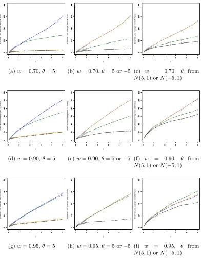
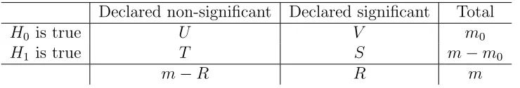
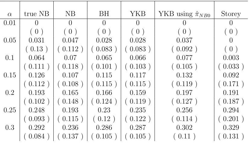
Figure 1.1 shows some representative plots which compare the average total loss
of the normal prior competitors under different sparsity and signal distribution
con-ditions when the signal is relatively strong. For this figure, the non-zero θi’s are
generated from the N(5,1) distribution, from a mixture of N(5,1) and N(−5,1)
distributions, or from a unit mass at the value 5. The proportion 1−ω of non-zero
θi’s is set to 0.05,0.10, and 0.30. The classifiers are compared at various values of
the cost constant c, which corresponds to the relative cost placed on false negative
results when signal is mistaken for noise. Our nonparametric classifier typically
out-performs the parametric competitors (i.e., has lower average loss) for broad ranges
of c values when the prior distribution is not specified correctly. In the graph, all
three classifiers were compared to a classification rule for which the correct prior
distribution was used. Similar simulation setups with weaker signal and higher
sig-nal sparsities were also tried. For weaker sigsig-nal, the performance of the parametric
111 11
11 11 1 1
1 1
1 1
0 1 2 3 4 5
0
100
200
300
400
22 2 2 22 2
2 22 2
2 2
2 2
0 1 2 3 4 5
0
100
200
300
400
3 3 3 3 33 3 3 3 3 3 3 3 3 3
0 1 2 3 4 5
0
100
200
300
400
4 4 4 4 4 44 4 4 4 4 4 4 4 4
0 1 2 3 4 5
0 100 200 300 400 c Empir
ical Loss (A
v
er
age o
v
er 100 Runs)
(a) w= 0.70, θ= 5
1 11 1 11 1 1 1 1
1 1
1 1 1
0 1 2 3 4 5
0
100
200
300
400
2222 2 2 22 2
2 2 2 2 2 2
0 1 2 3 4 5
0
100
200
300
400
333 3 33 3
3 33 3
3 3
3 3
0 1 2 3 4 5
0
100
200
300
400
4 4 4 44 4 4 4 4 4 4 4
4 4 4
0 1 2 3 4 5
0 100 200 300 400 c Empir
ical Loss (A
v
er
age o
v
er 100 Runs)
(b)w= 0.70,θ= 5 or −5
1 11 1 1 11 1 11
1 1
1 1 1
0 1 2 3 4 5
0
100
200
300
400
222 2 2 22 2
2 2 2 2 2 2 2
0 1 2 3 4 5
0
100
200
300
400
333 3 3 33 3
3 3 3 3 3 3 3
0 1 2 3 4 5
0
100
200
300
400
4 44 4 4 4 44 4 4
4
4 4
4 4
0 1 2 3 4 5
0 100 200 300 400 c Empir
ical Loss (A
v
er
age o
v
er 100 Runs)
(c) w = 0.70, θ from
N(5,1) orN(−5,1)
11 11 11 11 1 1 1 1 1 1 1
0 1 2 3 4 5
0 20 40 60 80 100 120 22 22
222 22 2
2 2
2 2
2
0 1 2 3 4 5
0 20 40 60 80 100 120
3 3 33 3 3 3 3 3 3 3
3 3
3 3
0 1 2 3 4 5
0 20 40 60 80 100 120
4 4 44 4 4 4 4
4 4 4 4
4 4 4
0 1 2 3 4 5
0 20 40 60 80 100 120 c Empir
ical Loss (A
v
er
age o
v
er 100 Runs)
(d)w= 0.90,θ= 5
11 1 11 11 1
1 1 1 1 1 1 1
0 1 2 3 4 5
0 20 40 60 80 100 120 22 22
2222 22 2 2 2 2 2
0 1 2 3 4 5
0 20 40 60 80 100 120 33 33
333 333
3 3
3 3
3
0 1 2 3 4 5
0 20 40 60 80 100 120
4 44 44 4 4 4 4 4 4
4 4 4 4
0 1 2 3 4 5
0 20 40 60 80 100 120 c Empir
ical Loss (A
v
er
age o
v
er 100 Runs)
(e)w= 0.90,θ= 5 or −5 11
11 11
111 1 1 1 1 1 1
0 1 2 3 4 5
0 20 40 60 80 100 120 22 22 22 222
2 2 2 2 2 2
0 1 2 3 4 5
0 20 40 60 80 100 120 33 33 33 33 33 3 3 3 3 3
0 1 2 3 4 5
0 20 40 60 80 100 120 44 44
444 4 4 4
4 4
4 4 4
0 1 2 3 4 5
0 20 40 60 80 100 120 c Empir
ical Loss (A
v
er
age o
v
er 100 Runs)
(f) w = 0.90, θ from
N(5,1) orN(−5,1)
111 1 11 11
1 1 1 1 1 1 1
0 1 2 3 4 5
0
20
40
60
80
222 2 22 2
2 22 2
2 2
2 2
0 1 2 3 4 5
0
20
40
60
80
3 33 3 3 3 3 3 3 3 3
3 3
3 3
0 1 2 3 4 5
0
20
40
60
80
4 44 4 44 4 4 4 4
4 4
4 4 4
0 1 2 3 4 5
0 20 40 60 80 c Empir
ical Loss (A
v
er
age o
v
er 100 Runs)
(g) w= 0.95, θ= 5
111 1 11 1
1 11 1
1 1
1 1
0 1 2 3 4 5
0 20 40 60 80 22 2 22 2
22 22 2
2 2
2 2
0 1 2 3 4 5
0
20
40
60
80
33 3 3 33 3
3 33 3
3 3
3 3
0 1 2 3 4 5
0
20
40
60
80
44 4 4 44 4 4 44 4
4 4 4 4
0 1 2 3 4 5
0 20 40 60 80 c Empir
ical Loss (A
v
er
age o
v
er 100 Runs)
(h)w= 0.95,θ= 5 or −5 11
11 111
11 1 1
1 1
1 1
0 1 2 3 4 5
0 20 40 60 80 22 22 22 22 22
2 2
2 2
2
0 1 2 3 4 5
0 20 40 60 80 33 333
333 3 3
3 3
3
3 3
0 1 2 3 4 5
0 20 40 60 80 44 444
444 4 4
4 4
4 4
4
0 1 2 3 4 5
0 20 40 60 80 c Empir
ical Loss (A
v
er
age o
v
er 100 Runs)
(i) w = 0.95, θ from
N(5,1) orN(−5,1)
1.6
Classification of Microarray Experiment
Out-put
Cellular organisms have internal biochemical mechanisms that help them to adjust to
changes in the surrounding environment by activating or repressing the expression of
certain parts of their genome in response to external changes. To better understand
which areas of an organism’s genome are involved in its response to outside factors,
researchers can use microarrrays to compare gene expression levels under various
conditions. In this section, we apply two of the classification rules described before,
the nonparametric and parametric with estimated mean and variance, to a publicly
available gene expression dataset.
Many observed differences in gene expression may indeed be due to the change
in conditions under investigation. Given the large number of genes involved and
the complexity of the genome, other changes in expression levels, however, may be
due to other factors. In identifying the part of the genome actually involved in
the organism’s response, classification algorithms which balance the costs of false
positives and false negatives can therefore be useful. As discussed above, the loss
function in (1.3.2) is readily interpretable in this context.
1.6.1
Gene Expression Data
When yeast cells experience harsh changes in their surroundings, they activate
in-ternal mechanisms to mitigate the stress. In the dataset, expression levels of several
chemical shocks to their environment. The data is collected using two-channel
mi-croarray techniques for multiple timepoints. The researchers measure changes in
expression levels at several times after the environmental shock and use statistical
techniques to cluster sets of genes with similar expression patterns to help identify
the parts of the yeast genome which are involved in various stress-response
mecha-nisms.
To illustrate the use of our classifiers, we focus on the data collected from just one
timepoint after a yeast colony has been subjected to an increase in hydrogen peroxide
concentration. We then work with the data as though all of the observations are
independent, as specified in model (1.2.1). In future work, we hope to extend our
nonparametric Bayes rule to deal with the richer time and dependence structure of
multiple timepoint microarray data.
1.6.2
Classification Results
The classification rules were tried on relative gene expression levels for one timepoint
in one of the microarray experiments (microarray y9-40, 10 minutes of exposure to
hydrogen peroxide) from the publicly available data. The gene expression data is
reported as “zero transformed” observations which summarize the gene expression
at each post-environmental change timepoint relative to expression levels before the
change. Positive (negative) values correspond to genes for which relative expression
levels were seen to go up (down) after the change to the environment. The classifiers
were then used to identify genes which are “sufficiently” over- or underexpressed
Observations are characterized as signal by a classifier if and only if they are in
a region where the ˆpi curve for the classifier is below the corresponding Bayes rule
threshold curve. Thus the decision rule for each classifier is characterized by the
relative gene expression levels at which its ˆpi curve crosses its Bayes rule threshold
curve. It was found that, for example, for c = 4, the nonparametric prior Bayes
procedure classifies all observations with relative expression levels outside the region
[−3.10,2.38] as signal. Forc= 4, the corresponding region for the parametric prior
rule is very slightly more conservative for the underexpressed genes and very slightly
less conservative for the overexpressed genes; it classifies the observations outside
of [−3.20,2.35] as signal. For c = 4, the classification results are extremely close,
with the nonparametric prior rule classifying 80 genes as differentially expressed as
compared to 79 for the parametric prior rule.
Results for other values of c were also obtained. For c = 10, for example, the
difference between the two classifiers becomes much more noticeable, with 153 signal
genes for the nonparametric prior classifier and 214 for the parametric prior rule.
It can be seen that, for reasonable values of c, the classification decisions provided
by the two rules in a particular dataset can vary greatly or overlap almost exactly
depending on the cost constant. At the same time, it should not be surprising that
there is less overlap in the decision rules for higher values ofcif, as is the case for this
dataset, most of the values are concentrated closer to 0, so that even small changes
1.7
Conclusion
In this chapter, we propose a Bayesian classifier in the context of a highly
inter-pretable loss function. While parametric Bayes classifiers may be conceptually
sim-pler, the nonparametric rule outperforms them in terms of the risk function when
the prior is not specified correctly. In particular, when the prior distribution is
misspecified for the parametric classifier, the nonparametric technique dominates
over the range of cvalues. This is reassuring because the particular choice of c is a
measure of the relative cost of false negatives to a researcher and, in practice, may
be difficult to specify precisely for some classification problems.
We illustrate the performance of two procedures using a publicly available gene
expression data set. It is seen that, while the decisions produced by the rules can be
similar, they can also vary greatly for reasonable values of the cost constant c. For
the gene expression application in this chapter, we focus on a single time point from
a multi-timepoint microarray experiment and treat the observations as if they were
independent. In future work, we hope to extend the nonparametric classification
Chapter 2
Classification Procedures based on
False Discovery Rates
2.1
Introduction
The simultaneous testing of multiple statistical hypotheses has been an active area
of research for many decades. The need to make many decisions at the same time
arises in the most diverse applications. One of the principal concerns of the multiple
testing literature is the search for useful criteria for evaluating statistical
decision-making techniques; given a criterion, techniques which satistfy it are necessary. In
this chapter, we focus on one such criterion, the False Discovery Rate, and propose
new ideas aimed at bounding it using nonparametric Bayesian techniques.
The False Discovery Rate (FDR) was introduced by Benjamini and Hochberg in
the papers that set up the main ideas that will be necessary for the sequel.
The FDR of a hypothesis testing procedure is defined as the expected proportion
of falsely rejected hyptoheses under the procedure given that at least one hypothesis
is rejected by it multiplied by the probability of rejecting at least one hypothesis.
Benjamini and Hochberg (1995) provided a so-called “linear step-up” procedure for
controlling the FDR at a desired level based on p-values for the case where the test
statistics from the hypotheses are independent. In subsequent work, Yekutieli and
Benjamini (2001) showed that the same p-value step-up procedure controls the FDR
for a broad class of dependence structures for the test statistics. Storey (2002; 2003)
focused on another criterion which had been highlighted by Benjamini and Hochberg
(1995) : the expected proportion of falsely rejected hypotheses given that at least
one hypothesis is rejected. Benjamini and Hochberg (1995) had ultimately rejected
this criterion, called positive FDR or pFDR by Storey (2002), in favor of the FDR
because the pFDR cannot be controlled in cases when all of the null hypotheses
are true. Yet, as Storey (2002) showed, if the test statistics are independent and if
it is assumed that whether each test statistic truly comes from the null hypothesis
or from the alternative can be thought of as binomial trials with some constant
probability of success, then the pFDR corresponding to the hypothesis rejection
region equals the probability that a hypothesis is null given that its test statistic
falls in the rejection region. This powerful connection makes the pFDR a natural
quantity to study in the Bayesian framework, and Storey (2002, 2003) proposes a
procedure that estimates this quantity for preselected rejection regions.
Bayes approach. The quantity of interest in their work was the probability that a
null hypothesis is true given the value of the associated test statistic. This
poste-rior probability was termed the local FDR since it was shown to be equivalent to
the FDR if the rejection region were restricted to a small (“local”) region around
this realized value of the test statistic. Efron et al. (2001) proposed one method
for estimating this posterior probability without parametric assumptions about the
alternative hypothesis distribution; other methods are, of course, also available, and
much of our later discussion focuses on studying the connection to FDR of the
nonparametric Bayes approach suggested by Raykar and Zhao (2010) .
The layout for this Chapter is as follows: in Section 2 of this Chapter, we begin
by discussing the FDR criterion as it was introduced by Benjamini and Hochberg
(1995). We then examine later work which built on the original formulation. We
look at the nonparametric prior procedure from the previous chapter and fit it within
this framework.
2.2
Multiple Hypothesis Testing and the False
Dis-covery Rate Criterion
In this section, we lay out a framework for studying binary classification and
intro-duce the notation used in this chapter (most of our notation follows the standard
notation in Benjamini and Hochberg (1995)). To discuss this problem, it will be
convenient to refer to a so-called “confusion matrix,” shown in Table 2.1, which
Table 2.1: A “confusion matrix” for multiple hypothesis testing
Declared non-significant Declared significant Total
H0 is true U V m0
H1 is true T S m−m0
m−R R m
table, m represents the total number of hypotheses being tested and m0 stands for
the number of truly null hypotheses among them. Given the data and a classification
procedure, the null hypothesis is rejected in R of the m hypothesis tests. Of the R
rejections,V are incorrect because they come from them0 hypothesis tests in which
the null hypothesis is in fact true. Similarly, there are T incorrect declarations of
non-significance for which the alternative hypothesis is actually true. Obviously, it
is desirable to have classificiation procedures for which bothV andT are small, but,
usually, trade-offs are necessary. Traditionally, in formulating multiple hypothesis
testing procedures, the focus has been on controlling the quantity P rob(V > 0),
which is called the family-wise error rate (FWER). For example, one well-known
approach which controls the FWER is the Bonferroni procedure (for extensive
ref-erences, see for example, Lehmann’s Testing Statistical Hypotheses (2005)). Quite
often, however, approaches which control the FWER are much more conservative
than needed for specific applications. For such cases, other criteria for evaluating
the performance of procedures for multiple hypothesis testing are available. One
especially popular criterion is the control of the so-called false discovery rate, or
FDR, as suggested by Benjamini and Hochberg (1995). We presently discuss the
2.2.1
The False Discovery Rate
The false discovery rate (FDR) was introduced by Benjamini and Hochberg (1995)
as a quantity to control for multiple hypothesis testing. The FDR is defined as
the expected proportion of incorrectly rejected hypotheses among all the rejected
hypotheses given that at least one ejection is made times the probability that at
least one rejection is made. That is
Definition:
F DR =E(V
R|R >0)P rob(R > 0) (2.2.1)
For many situations, this much less stringent error rate is more reasonable than the
FWER.
A procedure to control the FDR at a preset level α was also introduced in
Ben-jamini and Hochberg (1995). The procedure consists of ranking the p-values from
the m hypothesis tests and then comparing each of them, in order from smallest
to largest, to a constant that depends on the rank of the p-value, on m, and on
α. The first time a p-value exceeds the corresponding constant, the procedure is
stopped, with that p-value and all of the smaller p-values declared to belong to tests
in which the null hypothesis should be rejected. In other words, the procedure goes
as follows:
The Benjamini-Hochberg (1995) step-up procedure:
1. Rank from smallest to largest the p-values from the m tests. Denote the
resulting ordered list as p(1), p(2), ..., p(m) and denote the corresponding hypothesis
2. Let ˆk =max{i:p(i) ≤ miα}.
3. Reject the hypotheses H(1), ..., H(k) and accept the others.
Benjamini and Hochberg show that this procedure results in F DR≤ m0
mα≤α. It is important to emphasize that this procedure only provides “control” of an expected
quantity and not of the proportion of falsely rejected null hypotheses in a particular
sample, since the F DR is an expected value. Also, note that F DR is actually
controlled at a level which is typically more conservative than the stated level α. If
m0 were known, then the procedure could be made less conservative. Of course, m0
is unknown, but estimates of m0 or of the fraction m0/m can be made, and later
work by Storey (2002) and by Benjamini, Krieger, and Yekutieli (2006) shows that
less conservative procedures can be obtained by using estimates of these quanitites.
2.2.2
The pFDR criterion
A Bayesian framework for FDR was studied by Storey (2002, 2003). He reexamined
a quantity that had originally been considered and rejected in favor of FDR in the
work of Benjamini and Hochberg (1995) and showed that, under broadly applicable
assumptions, it is equivalent to the posterior probability that the null hypothesis
is true given that the associated test statistic falls in the rejection region. This
quantity is defined as the expected value of the fraction of false discoveries among
all the discoveries, given that at least one discovery has occurred; when no discoveries
be written as
pF DR=E
V
R|R >0
. (2.2.2)
Storey (2002, 2003) shows that when the sample consists of indpendent observations,
then the pFDR corresponds to the probability that a null hypothesis is true given
that it was declared false. Using Storey’s notation, this can be written as
pF DR(Γ) = P rob(H = 0|X ∈Γ), (2.2.3)
where H is a binary indicator for whether the null hypothesis is true, X is some
test statistic, and Γ stands for the rejection region. The formula can also be written
in terms of rejection regions for p-values, with hypotheses with test statistics that
have p-values in some interval [0, γ] being rejected. We can then rewrite the formula
above as
pF DR(γ) = π0P rob(p−value≤γ|H = 0)
P rob(p−value≤γ) . (2.2.4)
Storey (2002) proposes a technique for estimating the proportion π0 of true null
hypotheses, the probability P r(R >0) that at least one hypothesis is rejected, and
the pFDR associated with a particular rejection region [0, γ]:
ˆ
π0,Storey(λ) =
W(λ)
(1−λ)m, (2.2.5)
ˆ
P r(R >0) = R(γ)
and
pF DRλ(γ) =
ˆ
π0,Storey(λ)γ ˆ
P r(R >0)(1−(1−γ)m) (2.2.7)
where W(λ) is the number of p-values which exceed a tuning parameter λ, R(γ) is
the number of p-values that fall in the rejection interval [0, γ], and m is the total
number of hypotheses being tested.
Note that the last formula provides an estimator of pFDR for a rejection region
[0, γ] of p-values selected by the researcher. Storey (2002) shows that this estimator
has an upward bias for estimating the true pFDR of a rejection region. The
esti-mation approach can be contrasted against the more traditional aim of providing
procedures which control the error rate at a desired level α, such as the linear
step-up procedure of Benjamini and Hochberg (1995). In the next section, we discuss a
connection between FDR, pFDR, and empirical Bayes procedures. We then look at
ways of bounding pFDR using a nonparametric Bayesian approach.
2.3
Nonparametric Bayesian Classification and FDR
The FDR-controlling procedures described above rely on the explicit use of observed
p-values. We now change focus to a different approach which uses the posterior
prob-abilty that a null hypothesis is true given the value of the associated test statistic.
This quantity can be estimated using empirical Bayes techniques and the average
such posterior probability in a rejection region turns out to equal the pFDR of the
region, as discussed by Efron et al. (2001) and Efron (2005). The goal of this
between FDR and nonparametric Bayes techniques. A useful model for this setting
can be expressed as the mixture f of a null density f0 and an alternative density g
f(z) =π0f0(z) + (1−π0)g(z), (2.3.1)
Here, the symbolz stands for one-dimensional scores which are used for making the
binary classification decisions. For example, they may be transformed gene
expres-sion values from a large microarray experiment in which the goal is to determine
which genes change their expression levels (that is, they become overexpressed or
underexpressed) in response to a biologically interesting treatment, such as ioninzing
radiation. As discussed by Efron et al. (2001) , it is often the case that an
appro-priate data reduction technique must first be found to form the one-dimensional
statistics Z, since data on multiple characteristics for each unit of observation is
often available. Ways of reducing the data to single-dimenisonal summary
statis-tics are discussed in the paper, but these are not integral to our discussion in this
section. Here, we focus instead on the alternative methods for estimating posterior
probabilities.
Using Bayes’ Rule, the posterior probability of interest for the i0th observation zi
can be written as
1−pi(zi) = 1−π0f0/f(zi) (2.3.2)
and
where pi(zi) is the a posteori probability that the null hypothesis is true for an
obseration with summary score zi. In Efron et al. (2001) , this is called the local
FDR because, asymptotically, it is equivalent to the proportion of falsely rejected
hypotheses if the rejection region consists of test statistics close to zi. Note that
the expression on the right side of equation 2.3 has the same general form as the
quantity computed in 1.4.8 of Chapter 1. We look at this connection next.
Note that the mixture densityf can be estimated from the data, but this estimate
is not directly useful by itself if the density f0 is unknown. To remedy this, one can
make distributional assumptions or use permutations of the density f0, as is done,
for example, in Efron (2001), Efron (2005), Raykar and Zhao (2010), and other work
where some prior distribution is assumed for the null density f0.
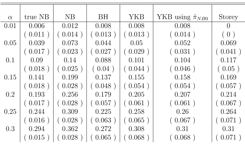
2.4
Simulation Results
Our work compares the empirical false discovery proportionV /Rfor various
classifi-cation rules. We report the results of several simulations here. For each simulation,
500 observations were generated from two distributions, the null hypothesis
distribu-tion N(0,1) and some alternative hypothesis distribudistribu-tion. The false discovery rates
associated with several different classification rules were then computed. For each
combination of null and alternative hypothesis distributions, these computations
were repeated for 100 samples of 500 observations. We performed computations for
each of the significance levels (α) reported in the first column of the table. In the
when using the nonparametric Bayes rule at each significance level α with true
val-ues of g and π0 plugged in. In the third column, we use the same rule, but with
estimates of g and π0 plugged in. The averages in this third column are computed
in the following way:
Algorithm 3.1
The non-parametric prior empirical Bayes rule for significance level α.
1. For each observation zi, compute the estimate ˆpiN B(zi) for the posterior
proba-bility P rob(βi = 0|zi,z) using the formula
ˆ
piN B(zi) =
ˆ
π0φ(zi) ˆ
π0φ(zi) + (1−πˆ0)ˆg(zi)
, (2.4.1)
where ˆπ0 stands for the estimate of π0 =P rob(βi = 0), ˆg(zi) is an estimate of the
marginal density ofzi given that βi 6= 0, andφ(zi) is the value of theN(0,1) density
at zi.
2. Order the values ˆpN B(zi) computed in Step 1 from smallest to largest and
denote the ordered list as {pˆ(1), ...,pˆ(m)}and let x(j) stand for the observation from
Step 1 that is associated with the j’th largest ˆp (and NOT for the j’th largest zi).
Let
K =max{k s.t.
k
X
j=1 ˆ
p(k)/k ≤α}. (2.4.2)
Classify the observations x(j) as having come from the alternative distribution for
j ≤K and from the null distribution for all other j.
rejections when using the original linear step-up Benjamini and Hochberg (1995)
procedure. The fifth column of each table shows the results for the two-stage version
of the step-up procedure introduced in Benjamini, Krieger, and Yekutieli (2006), in
which the ratio m0/m of true null hypotheses is estimated. The sixth column has
results for an ad hoc version of the two-stage step up procedure of the fifth column in
which ˆπ0,N B is used to estimate the ratiom0/m. Finally, the seventh column presents
results based on the estimates of pFDR from Storey (2002). As noted above, the
procedure in Storey (2002) is unlike the other approaches in the sense that it provides
estimates of an error rate for predetermined rejection intervals instead of providing
rejection intervals for desired error levels of an error rate. To make the procedures
comparable, we compute the Storey (2002) estimate of pFDR for each observation
and reject the null hypothesis for all observations for this estimate falls below the
desired level α.
2.5
Discussion of Simulation Results
The aim for methods that focus on the FDR and pFDR is usually a slight
conser-vative bias in expectation. In other words, the goal is typically to come up with
procedures for which the expected value of the error rate in question falls below the
nominal significance levelα. For example, the linear step-up procedure proposed by
Benjamini and Hochberg (1995) controls the FDR, which is defined as the expected
value in (3.3.6), below the desired nominal rateα. In fact, the control for this
proce-dure is at the more conservative rate m0
Table 2.2: Average empirical V /R, testing βi = 0 against βi = 2, π0=0.9
α true NB NB BH YKB YKB using ˆπN B0 Storey
0.01 0 0 0.003 0.003 0.003 0
( 0 ) ( 0 ) ( 0.033 ) ( 0.033 ) ( 0.033 ) ( 0 )
0.05 0.026 0.038 0.037 0.037 0.039 0
( 0.067 ) ( 0.078 ) ( 0.091 ) ( 0.09 ) ( 0.092 ) ( 0 )
0.1 0.086 0.081 0.066 0.066 0.085 0.007
( 0.078 ) ( 0.082 ) ( 0.097 ) ( 0.097 ) ( 0.099 ) ( 0.052 )
0.15 0.133 0.117 0.118 0.12 0.139 0.104
( 0.072 ) ( 0.085 ) ( 0.108 ) ( 0.11 ) ( 0.122 ) ( 0.192 )
0.2 0.186 0.146 0.174 0.178 0.205 0.192
( 0.074 ) ( 0.083 ) ( 0.123 ) ( 0.125 ) ( 0.125 ) ( 0.206 )
0.25 0.238 0.184 0.222 0.224 0.248 0.281
( 0.072 ) ( 0.087 ) ( 0.115 ) ( 0.116 ) ( 0.113 ) ( 0.174 )
0.3 0.29 0.23 0.269 0.276 0.307 0.324
( 0.072 ) ( 0.088 ) ( 0.117 ) ( 0.122 ) ( 0.115 ) ( 0.137 )
Table 2.3: Average empirical V /R, testing βi = 0 against βi = 2 or −2, π0=0.9
α true NB NB BH YKB YKB using ˆπN B0 Storey
0.01 0 0 0 0 0 0
( 0 ) ( 0 ) ( 0 ) ( 0 ) ( 0 ) ( 0 )
0.05 0.031 0.047 0.028 0.028 0.037 0
( 0.13 ) ( 0.112 ) ( 0.083 ) ( 0.083 ) ( 0.092 ) ( 0 )
0.1 0.064 0.07 0.065 0.066 0.077 0.003
( 0.111 ) ( 0.118 ) ( 0.101 ) ( 0.103 ) ( 0.105 ) ( 0.033 )
0.15 0.126 0.107 0.115 0.117 0.132 0.092
( 0.112 ) ( 0.108 ) ( 0.115 ) ( 0.115 ) ( 0.119 ) ( 0.171 )
0.2 0.193 0.165 0.166 0.159 0.197 0.191
( 0.102 ) ( 0.148 ) ( 0.124 ) ( 0.119 ) ( 0.127 ) ( 0.187 )
0.25 0.248 0.193 0.23 0.235 0.256 0.294
( 0.093 ) ( 0.115 ) ( 0.12 ) ( 0.122 ) ( 0.114 ) ( 0.201 )
0.3 0.292 0.236 0.286 0.287 0.302 0.329
Table 2.4: Average empirical V /R, testing βi = 0 against βi from 0.5N(2,1) + 0.5N(−2,1), π0=0.9
α true NB NB BH YKB YKB using ˆπN B0 Storey
0.01 0.002 0.006 0.006 0.006 0.008 0
( 0.017 ) ( 0.034 ) ( 0.034 ) ( 0.034 ) ( 0.036 ) ( 0 )
0.05 0.042 0.041 0.038 0.04 0.04 0
( 0.078 ) ( 0.078 ) ( 0.072 ) ( 0.073 ) ( 0.072 ) ( 0 )
0.1 0.088 0.08 0.085 0.087 0.093 0.052
( 0.076 ) ( 0.087 ) ( 0.084 ) ( 0.086 ) ( 0.085 ) ( 0.126 )
0.15 0.144 0.126 0.137 0.142 0.153 0.167
( 0.079 ) ( 0.085 ) ( 0.085 ) ( 0.086 ) ( 0.087 ) ( 0.136 )
0.2 0.194 0.169 0.183 0.188 0.2 0.224
( 0.07 ) ( 0.084 ) ( 0.086 ) ( 0.088 ) ( 0.087 ) ( 0.107 )
0.25 0.249 0.208 0.232 0.238 0.247 0.277
( 0.076 ) ( 0.09 ) ( 0.095 ) ( 0.096 ) ( 0.1 ) ( 0.108 )
0.3 0.307 0.258 0.271 0.29 0.312 0.33
( 0.067 ) ( 0.085 ) ( 0.1 ) ( 0.099 ) ( 0.095 ) ( 0.108 )
Table 2.5: Average empirical V /R, testing βi = 0 against βi = 5, π0=0.9
α true NB NB BH YKB YKB using ˆπN B0 Storey
0.01 0.006 0.012 0.008 0.008 0.008 0
( 0.011 ) ( 0.014 ) ( 0.013 ) ( 0.013 ) ( 0.014 ) ( 0 )
0.05 0.039 0.073 0.044 0.05 0.052 0.069
( 0.017 ) ( 0.023 ) ( 0.027 ) ( 0.029 ) ( 0.031 ) ( 0.041 )
0.1 0.09 0.14 0.088 0.101 0.104 0.117
( 0.018 ) ( 0.025 ) ( 0.04 ) ( 0.044 ) ( 0.046 ) ( 0.05 )
0.15 0.141 0.199 0.137 0.155 0.158 0.169
( 0.018 ) ( 0.028 ) ( 0.048 ) ( 0.054 ) ( 0.054 ) ( 0.057 )
0.2 0.193 0.256 0.179 0.205 0.207 0.214
( 0.017 ) ( 0.028 ) ( 0.057 ) ( 0.061 ) ( 0.061 ) ( 0.067 )
0.25 0.244 0.309 0.225 0.258 0.26 0.264
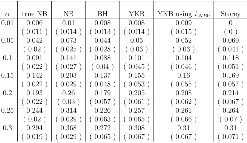
( 0.016 ) ( 0.028 ) ( 0.063 ) ( 0.065 ) ( 0.067 ) ( 0.071 )
0.3 0.294 0.362 0.272 0.308 0.31 0.31
Table 2.6: Average empirical V /R, testing βi = 0 against βi = 5 or −5, π0=0.9
α true NB NB BH YKB YKB using ˆπN B0 Storey
0.01 0.006 0.01 0.008 0.008 0.009 0
( 0.011 ) ( 0.014 ) ( 0.013 ) ( 0.014 ) ( 0.015 ) ( 0 )
0.05 0.042 0.073 0.044 0.05 0.052 0.069
( 0.02 ) ( 0.025 ) ( 0.028 ) ( 0.03 ) ( 0.03 ) ( 0.041 )
0.1 0.091 0.141 0.088 0.101 0.104 0.118
( 0.022 ) ( 0.027 ) ( 0.04 ) ( 0.045 ) ( 0.046 ) ( 0.051 )
0.15 0.142 0.203 0.137 0.155 0.16 0.169
( 0.022 ) ( 0.029 ) ( 0.048 ) ( 0.053 ) ( 0.055 ) ( 0.057 )
0.2 0.193 0.26 0.179 0.205 0.208 0.214
( 0.022 ) ( 0.03 ) ( 0.057 ) ( 0.061 ) ( 0.062 ) ( 0.067 )
0.25 0.244 0.314 0.226 0.257 0.261 0.264
( 0.02 ) ( 0.029 ) ( 0.063 ) ( 0.065 ) ( 0.066 ) ( 0.07 )
0.3 0.294 0.368 0.272 0.308 0.31 0.31
( 0.019 ) ( 0.029 ) ( 0.065 ) ( 0.067 ) ( 0.067 ) ( 0.071 )
and Yekutieli (2006) refines the original approach to make the control in expectation
less conservative by estimating m0/m. Similarly, Storey (2002, 2003) shows that, in
expectation, his estimator overshoots the true pFDR of a fixed rejection region.
On the other hand, as far as we know, there are no procedures that control the
Bayes posterior probabilitiespior their averages in expectation. The current absence
of such procedures may be seen as a weakness of using posterior probabilitites
es-timated by nonparametric Bayes approaches for working with false discovery rates.
And yet, if the estimates of pi are good, this approach seems reasonable and
of-fers greater flexibility for interpretation, as argued by Efron et al. (2001), because
estimates of posterior probabilities are provided for each tested hypothesis.
were falsely rejected among all the declared rejections. In tables 2.2-2.6, we report
the empirical average and empirical standard deviation of this proportion for
sev-eral different classification procedures. The second column in these tables (labeled
as “true NB”) reports results for the nonparametric Bayes procedure with true
marginal density g and true population proportion π0. Not surprisingly, this
col-umn gives excellent results in the sense that the averages fall just below the stated
significance levels α and the empirical standard deviations are the lowest in the
ta-bles. Of course, the trueg andπ0 are unknown and must be estimated. This is done
in the next column, labeled NB, using the estimates ofg and π0 provided by Raykar
and Zhao (2010a). Reassuringly, this column gives results which are quite close to
the results for the classification procedure which uses the true g and π0 for much of
the time. Interestingly, the simulation results for this procedure are better for the
harder classification problems described in tables 2.2-2.4 than in the relatively easier
ones in tables 2.5 and 2.6; for the latter set-ups, the nonparametric Bayes procedure
rejects too many hypotheses. A similar pattern is seen for the classification
proce-dures described in the fifth and sixth columns, which correspond to two different
versions of the linear step-up procedure for which the population proportion π0 of
null hypotheses is estimated. The results in the fourth column of each table are
for the original Benjamini and Hochberg (1995) procedure. The empirical average
results in this column always fall below the stated level α, but the nonparametric
Bayes results are often better for small values of α.
The results in the last column were produced using the estimator of pFDR that
(2002), but using two-sided p-values). Because the procedure described in Storey’s
work is an estimator of pFDR for fixed rejection regions and the other procedures
used in the simultations are instead ways of limiting pFDR given the desired
signif-icance level, Storey’s approach is not directly comparable to the others. To make it
comparable, we first use it to compute estimates of pFDR for every hypothesis and
then reject the hypotheses for which these estimates fall below the deisred level α.
The results using this procedure seem to be too conservative for smaller values of α
Chapter 3
A Recalibration Procedure which
maximizes the AUC: A Use-Case
for Binormal Assumtions
3.1
Introduction and Related Work
Most binary classifiers make their final decision as to whether an instance is positive
or negative based on a scalar score, which is computed as a function of the features
corresponding to that instance. The popular and widely used procedure chooses
a single threshold value on the score scale and assigns the positive label (1) to
observations with scores that fall above this value and the negative label (0) to
threshold can then be written as
δ(x) =
1 if f(x)≥θ
0 otherwise
, (3.1.1)
where f(x) is the raw score computed as a function f for an instance x∈Rd (the
d-dimensional feature vector) and θ is an appropriately chosen threshold parameter.
This thresholding rule is essentially built on the assumption that a larger scoref(x)
provides a larger chance of y= 1.
One popular way of evaluating the performance of such binary classification rules
is to use the Receiver Operating Characteristic (ROC) curve. There are connections
between binary regression generalized linear models and ROC curves (Pepe, 2000).
The ROC curve essentially is a plot of thesensitivity on the y-axis and1-specificity
on the x-axis. Each threshold θ corresponds to a point on the ROC plot and the
ROC curve is obtained asθis swept from−∞to∞. Classifiers that simultaneously
have higher sensitivity and higher specificity are more desirable and dominate their
competitors. In practice, however, one usually finds several classifiers with
inter-secting ROC curves. One popular procedure selects the classifier with the highest
area under its ROC curve (AUC).
In this chapter we focus on a raw score recalibration procedure that can maximize
the AUC for thresholding rules under certain assumptions. We do not dwell on
the particular classifier used, as the recalibration we propose can be used with
any general black-box classifier which uses scores to make a final decision. Area