Volume 16, Number 5 (2018), 733-750
URL:https://doi.org/10.28924/2291-8639 DOI:10.28924/2291-8639-16-2018-733
CUBIC GRAPHS WITH APPLICATION
SHEIKH RASHID1, NAVEED YAQOOB2,∗, MUHAMMAD AKRAM3, MUHAMMAD GULISTAN1
1Department of Mathematics, Hazara University, Mansehra, Pakistan
2Department of Mathematics, College of Science Al-Zulfi, Majmaah University, Al-Zulfi, Saudi Arabia
3Department of Mathematics, University of the Punjab, New Campus, Lahore, Pakistan
∗Corresponding author: [email protected]
Abstract. We introduce certain concepts, including cubic graphs, internal cubic graphs, external cubic graphs, and illustrate these concepts by examples. We deal with fundamental operations, Cartesian product, composition, union and join of cubic graphs. We discuss some results of internal cubic graphs and external cubic graphs. We also describe an application of cubic graphs.
1. Introduction
Cubic sets are one of the real generalizations of fuzzy sets [27] provided by Jun et al. [9–11,15,26] during
the last five years. They developed cubic set theory in many directions and for more detail about cubic sets
one can see [12]. Kang and Kim [13] studied mappings of cubic sets. Muhiuddin et al. [18] presented the
idea of stable cubic sets.
Fuzzy graphs were studied by Rosenfeld [23] and give a few theoretical ideas in spite of the fact that the
fundamental thought was presented by Kauffmann [14] in 1973. Bhattacharya [6] gave some remarks on
fuzzy graphs. A book written by Mordeson and Nair [17] is devoted especially to the study of fuzzy graphs
Received 2018-03-13; accepted 2018-05-22; published 2018-09-05. 2010Mathematics Subject Classification. 68R10, 05C72.
Key words and phrases. cubic sets; cubic graphs; internal and external cubic graphs.
c
2018 Authors retain the copyrights of their papers, and all open access articles are distributed under the terms of the Creative Commons Attribution License.
and fuzzy hypergraphs. Akram et al. gave the idea of interval-valued fuzzy graphs [1,2], intuitionistic fuzzy
graphs [3] and bipolar fuzzy graphs [4,5]. Borzooei and Rashmanlou [7] studied Cayley interval-valued
fuzzy threshold graphs. Buckley [8] introduced self-centered graphs. Sunitha et al. [25] characterized g-self
centered fuzzy graphs. Mishra et al. [16] studied coherent category of interval-valued intuitionistic fuzzy
graphs. Pal et al. [19] and Pramanik et al. [21,22] added some useful results to the theory of interval-valued
fuzzy graphs. Parvathi et al. [20] provided some different operations on intuitionistic fuzzy graphs and Sahoo
and Pal [24] studied product of intuitionistic fuzzy graphs.
In this paper we study some operations on cubic graphs. Internal and external cubic graphs are studied
with some example. We provided some conditions for union and join of external and internal cubic graphs.
2. Preliminaries
Here we recall some basic helping material from the existing literature.
Definition 2.1. A graph is denoted by Ω∗= (P, Q),whereP denotes the set of vertices of Ω∗ andQstands
for the set of edges of Ω∗.
Definition 2.2. [12] LetT be a non-empty set. By a cubic set in T we mean a structure
Λ ={ht,$eΛ(t), µΛ(t)i |t∈T}
in which$eΛis an interval-valued fuzzy set inT andµΛ is a fuzzy set inT.
A cubic set Λ ={ht,$eΛ(t), µΛ(t)i |t∈T}is simply denoted by Λ =h$eΛ, µΛi.
Definition 2.3. [12] LetT be a non-empty set. A cubic set Λ =h$eΛ, µΛiin T is said to be an internal cubic (resp., external cubic) set if
$−Λ(t)≤µΛ(t)≤$+Λ(t) (resp.,µΛ(t)∈/ ($−Λ(t), $+Λ(t)))
for allt∈T.
Definition 2.4. [12] For any Λi={ht,$eΛi(t), µΛi(t)i |t∈T}wherei∈I,we define
(a)∪P i∈I
Λi=
t,
∪ i∈I$eΛi
(t),
∨ i∈IµΛi
(t)
|t∈T
(P-union)
(b)∪R i∈I
Λi=
t,
∪ i∈I$eΛi
(t),
∧ i∈IµΛi
(t)
|t∈T
(R-union)
3. Cubic graphs
Definition 3.1. Let M∗ = hP, Qi be a graph. A cubic graph of a graph M∗ = hP, Qi, is the structure
M =hα, βi,where α=h$eα, µαiis the cubic set representation for the vertexP andβ =h$eβ, µβidenotes
the cubic set representation for the edgeQ, with
e
$α : P →D[0,1], µα:P →[0,1],
and $eβ : Q→D[0,1], µβ :Q→[0,1],
such that
e
$β(pipj) rmin{$eα(pi),$eα(pj)},
µβ(pipj) ≤ max{µα(pi), µα(pj)},
for all (pi, pj)∈Q⊆P×P.
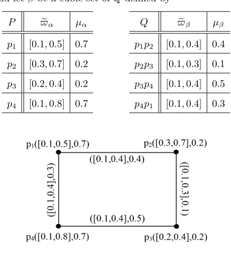
Example 3.1. Let us consider a graph Ω∗= (P, Q) such thatP ={p1, p2, p3, p4},Q={p1p2, p2p3, p3p4, p4p1}. Letαbe a cubic set of P and letβ be a cubic set ofQdefined by
P $eα µα
p1 [0.1,0.5] 0.7
p2 [0.3,0.7] 0.2
p3 [0.2,0.4] 0.2
p4 [0.1,0.8] 0.7
Q $eβ µβ
p1p2 [0.1,0.4] 0.4
p2p3 [0.1,0.3] 0.1
p3p4 [0.1,0.4] 0.5
p4p1 [0.1,0.4] 0.3
Figure 1. Cubic graph
By routine calculations, it can be observed that the graph shown in Fig. 1 is a cubic graph.
Example 3.2. Consider a graph Ω∗= (P, Q).Letαbe a cubic set ofP and letβbe a cubic set ofQdefined by
µα(pi) =
$−α(pi) +$α+(pi)
2 and µβ(ei) =
$β−(ei) +$+β(ei)
2 .
Remark 3.1. If$eβ(pipj) = [0,0] andµβ(pipj) = 0,then the cubic graphM =hα, βihas no edge.
Definition 3.2. Let M1 = hα1, β1i and M2 = hα2, β2i be two cubic graphs of the graphs Ω∗1 and Ω∗2, respectively. The Cartesian product of M1 and M2 is denoted by M1×M2 = hα1×α2, β1×β2i and is defined as follows:
(i)
($eα1×$eα2)(p1, p2) =rmin{$eα1(p1),$eα2(p2)}
(µα1×µα2)(p1, p2) = max{µα1(p1), µα2(p2)}
for all (p1, p2)∈P=P1×P2,
(ii)
($eβ1×$eβ2)((q, q2)(q, p2)) =rmin{$eα1(q),$eβ2(q2p2)}
(µβ1×µβ2)((q, q2)(q, p2)) = max{µα1(q), µβ2(q2p2)}
for allq∈P1, and q2p2∈Q2,
(iii)
($eβ1×$eβ2)((q1, r)(p1, r)) =rmin{$eβ1(q1p1),$eα2(r)}
(µβ1×µβ2)((q1, r)(p1, r)) = max{µβ1(q1p1), µα2(r)}
for allr∈P2, andq1p1∈Q1.
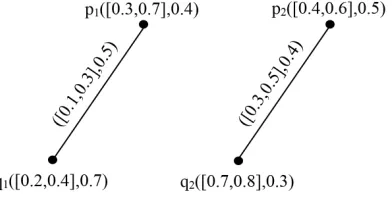
Example 3.3. Consider two cubic graphsM1=hα1, β1iandM2=hα2, β2ias shown in figure2.
Figure 2. Cubic graphsM1andM2
Then, their corresponding Cartesian productM1×M2 is shown in figure3.
Figure 3. Cubic graphM1×M2
Clearly,M1×M2is a cubic graph.
Proof. The conditions forα1×α2 are obvious, therefore, we verify only conditions forβ1×β2. Letq∈P1, andq2p2∈Q2. Then
($eβ1×$eβ2)((q, q2)(q, p2)) = rmin{$eα1(q),$eβ2(q2p2)}
rmin{$eα1(q), rmin{$eα2(q2),$eα2(p2)}}
= rmin{rmin{$eα1(q),$eα2(q2)}, rmin{$eα1(q),$eα2(p2)}}
= rmin{($eα1×$eα2)(q, q2),($eα1×$eα2)((q, p2)}
(µβ1×µβ2)((q, q2)(q, p2)) = max{µα1(q), µβ2(q2p2)}
≤ max{µα1(q),max{µα2(q2), µα2(p2)}}
= max{max{µα1(q), µα2(q2)},max{µα1(q), µα2(p2)}}
= max{(µα1×µα2)(q, q2),(µα1×µα2)((q, p2)}
Similarly, we can prove it forr∈P2, andq1p1∈Q1.
Definition 3.3. Let M1 = hα1, β1i and M2 = hα2, β2i be two cubic graphs of the graphs Ω∗1 and Ω∗2, respectively. The composition of M1 and M2 is denoted by M1[M2] =hα1◦α2, β1◦β2i and is defined as follows:
(i)
($eα1◦$eα2)(p1, p2) =rmin{$eα1(p1),$eα2(p2)}
(µα1◦µα2)(p1, p2) = max{µα1(p1), µα2(p2)}
for all (p1, p2)∈P=P1×P2,
(ii)
($eβ1◦$eβ2)((q, q2)(q, p2)) =rmin{$eα1(q),$eβ2(q2p2)}
(µβ1◦µβ2)((q, q2)(q, p2)) = max{µα1(q), µβ2(q2p2)}
for allq∈P1, and q2p2∈Q2, (iii)
($eβ1◦$eβ2)((q1, r)(p1, r)) =rmin{$eβ1(q1p1),$eα2(r)}
(µβ1◦µβ2)((q1, r)(p1, r)) = max{µβ1(q1p1), µα2(r)}
for allr∈P2, andq1p1∈Q1.
(iv)
($eβ1◦$eβ2)((q1, q2)(p1, p2)) =rmin{$eα2(q2),$eα2(p2),$eβ1(q1p1)}
(µβ1◦µβ2)((q1, q2)(p1, p2)) = max{µα2(q2), µα2(p2), µβ1(q1p1)}
for allq2, p2∈P2, q2=6 p2 andq1p1∈Q1.
Figure 4. Cubic graphM1[M2]
Clearly,M1[M2] is a cubic graph.
Proposition 3.2. The composition of two cubic graphs is a cubic graph.
Definition 3.4. Let M1 = hα1, β1i and M2 = hα2, β2i be two cubic graphs of the graphs Ω∗1 and Ω∗2, respectively. TheP-union of two cubic graphsM1 andM2 is denoted byM1∪PM2=hα1∪pα2, β1∪pβ2i and is defined as follows:
(i) ($eα1∪p$eα2)(p) =
e
$α1(p) ifp∈P1−P2
e
$α2(p) ifp∈P2−P1
rmax{$eα1(p),$eα2(p)} ifp∈P1∩P2
(ii) (µα1∪pµα2)(p) =
µα1(p) ifp∈P1−P2
µα2(p) ifp∈P2−P1
max{µα1(p), µα2(p)} ifp∈P1∩P2
(iii) ($eβ1∪p$eβ2)(pipj) =
e
$β1(pipj) ifpipj ∈Q1−Q2
e
$β2(pipj) ifpipj ∈Q2−Q1
rmax{$eβ1(pipj),$eβ2(pipj)} ifpipj ∈Q1∩Q2
(iv) (µβ1∪pµβ2)(pipj) =
µβ1(pipj) ifpipj∈Q1−Q2
µβ2(pipj) ifpipj∈Q2−Q1
max{µβ1(pipj), µβ2(pipj)} ifpipj∈Q1∩Q2
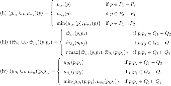
Definition 3.5. Let M1 = hα1, β1i and M2 = hα2, β2i be two cubic graphs of the graphs Ω∗1 and Ω∗2, respectively. TheR-union of two cubic graphsM1 andM2 is denoted byM1∪RM2=hα1∪Rα2, β1∪Rβ2i and is defined as follows:
(i) ($eα1∪R$eα2)(p) =
e
$α1(p) ifp∈P1−P2
e
$α2(p) ifp∈P2−P1
(ii) (µα1∪Rµα2)(p) =
µα1(p) ifp∈P1−P2
µα2(p) ifp∈P2−P1
min{µα1(p), µα2(p)} ifp∈P1∩P2
(iii) ($eβ1∪R$eβ2)(pipj) =
e
$β1(pipj) ifpipj ∈Q1−Q2
e
$β2(pipj) ifpipj ∈Q2−Q1
rmax{$eβ1(pipj),$eβ2(pipj)} ifpipj ∈Q1∩Q2
(iv) (µβ1∪Rµβ2)(pipj) =
µβ1(pipj) ifpipj∈Q1−Q2
µβ2(pipj) ifpipj∈Q2−Q1
min{µβ1(pipj), µβ2(pipj)} ifpipj∈Q1∩Q2
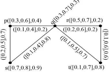
Example 3.5. Consider two cubic graphsM1=hα1, β1iandM2=hα2, β2ias shown in figure5.
Figure 5. Cubic graphsM1andM2
Then, their correspondingP-unionM1∪P M2 is shown in figure6.
Figure 6. Cubic graphM1∪P M2
Figure 7. Cubic graphM1∪RM2
Clearly,M1∪PM2 andM1∪RM2 are cubic graphs.
Proposition 3.3. TheP-union andR-union of two cubic graphs is a cubic graph.
Proof. Since all the conditions forα1∪pα2are automatically satisfied therefore, we verify only conditions forβ1∪pβ2. In the case, whenqp∈Q1∩Q2. Then
($eβ1∪p$eβ2)(qp) =rmax{$eβ1(qp),$eβ2(qp)}
rmax{rmin{$eα1(q),$eα1(p)}, rmin{$eα2(q),$eα2(p)}}
=rmin{rmax{$eα1(q),$eα2(q)}, rmax{$eα1(p),$eα2(p)}}
=rmin{($eα1∪p$eα2)(q),($eα1∪p$eα2)(p)}.
(µβ1∪pµβ2)(qp) = max{µβ1(qp), µβ2(qp)}
≤max{max{µα1(q), µα1(p)},max{µα2(q), µα2(p)}}
= max{max{µα1(q), µα2(q)},max{µα1(p), µα2(p)}}
= max{(µα1∪pµα2)(q),(µα1∪pµα2)(p)}.
Ifqp∈Q1andqp /∈Q2, then
($eβ1∪p$eβ2)(qp) rmin{($eα1∪p$eα2)(q),($eα1∪p$eα2)(p)}
(µβ1∪pµβ2)(qp) ≤ max{(µα1∪pµα2)(q),(µα1∪pµα2)(p)}.
Ifqp∈Q2andqp /∈Q1, then
($eβ1∪p$eβ2)(qp) rmin{($eα1∪p$eα2)(q),($eα1∪p$eα2)(p)}
Hence theP-union of two cubic graphs is a cubic graph. The case forR-union of two cubic graphs can be
seen in a similar way.
Definition 3.6. Let M1 = hα1, β1i and M2 = hα2, β2i be two cubic graphs of the graphs Ω∗1 and Ω∗2, respectively. The P-join of two cubic graphs M1 and M2 is denoted by M1+P M2 =hα1+P α2, β1+Pβ2i and is defined as follows:
(i)
($eα1+P$eα2)(p) = ($eα1∪P$eα2)(p)
(µα1+P µα2)(p) = (µα1∪P µα2)(p)
forp∈P1∪P2,
(ii)
($eβ1+P$eβ2)(qp) = ($eβ1∪P$eβ2)(qp)
(µβ1+P µβ2)(qp) = (µβ1∪Pµβ2)(qp)
forqp∈Q1∩Q2,
(iii)
($eβ1+P $eβ2)(qp) =rmin{$eα1(q),$eα2(p)}
(µβ1+P µβ2)(qp) = min{µα1(q), µα2(p)}
forqp∈Q∗, whereQ∗is the set of all edges joining the vertices of P1 andP2.
Definition 3.7. Let M1 = hα1, β1i and M2 = hα2, β2i be two cubic graphs of the graphs Ω∗1 and Ω∗2, respectively. The R-join of two cubic graphs M1 and M2 is denoted by M1+RM2 =hα1+Rα2, β1+Rβ2i and is defined as follows:
(i)
($eα1+R$eα2)(p) = ($eα1∪R$eα2)(p)
(µα1+Rµα2)(p) = (µα1∪Rµα2)(p)
forp∈P1∪P2,
(ii)
($eβ1+R$eβ2)(qp) = ($eβ1∪R$eβ2)(qp)
(µβ1+Rµβ2)(qp) = (µβ1∪Rµβ2)(qp)
forqp∈Q1∩Q2,
(iii)
($eβ1+R$eβ2)(qp) =rmin{$eα1(q),$eα2(p)}
(µβ1+Rµβ2)(qp) = max{µα1(q), µα2(p)}
forqp∈Q∗, whereQ∗is the set of all edges joining the vertices of P1 andP2.
Example 3.6. Consider two cubic graphsM1=hα1, β1iandM2=hα2, β2ias shown in figure8.
Then, their correspondingP-joinM1+PM2is shown in figure 9.
Figure 9. Cubic graphM1+P M2
Also, their correspondingR-join M1+RM2 is shown in figure10.
Figure 10. Cubic graphM1+RM2
Clearly,M1+PM2andM1+RM2 are cubic graphs.
Proposition 3.4. TheP-join andR-join of two cubic graphs is a cubic graph.
4. Internal and external cubic graphs
Here in this section we discuss some results related with internal and external cubic graphs.
Definition 4.1. A cubic graphM =hα, βiis said to be an
(i) internal cubic graph (IC-graph) if
for eachpi∈P andei∈Q.
(ii) external cubic graph (EC-graph) if
µα(pi)∈/($α−(pi), $+α(pi)) and µβ(ei)∈/($β−(ei), $β+(ei))
for eachpi∈P andei∈Q.
Example 4.1. The cubic graphsM1 =hα1, β1iand M2=hα2, β2iare internal and external cubic graphs, respectively, as shown in figure11.
Figure 11. IC-graphM1and EC-graph M2
Theorem 4.1. Let{Mi=hαi, βii |i∈I}be a family of IC-graphs. Then∪P i∈I
Mi is an IC-graph.
Proof. SinceMiis an IC-graph, we have$α−(p)≤µα(p)≤$+α(p) and$ −
β(e)≤µβ(e)≤$β+(e) fori∈I. This implies that
∪ i∈I$
− α
(p)≤
∨ i∈Iµα
(p)≤
∪ i∈I$
+ α
(p),
and
∪ i∈I$
− β
(e)≤
∨ i∈Iµβ
(e)≤
∪ i∈I$
+ β
(e).
Hence∪P i∈I
Mi is an IC-graph.
The following example shows that theR-union of IC-graphs need not be an IC-graph (EC-graph).
Figure 12. IC-graphsM1 andM2
Then, their correspondingR-unionM1∪RM2is shown in figure 13.
Figure 13. R-union of IC-graphsM1 andM2
It is easy to see that the cubic graphM1∪RM2 is neither IC-graph nor EC-graph.
We provide a condition for theR-union of two IC-graphs to be an IC-graph.
Theorem 4.2. LetM1=hα1, β1iandM2=hα2, β2ibe IC-graphs such that
max{$α−1(p), $−α2(p)} ≤min{µα1(p), µα2(p)}
and
max{$β−
1(e), $
−
β2(e)} ≤min{µβ1(e), µβ2(e)}
for allp∈P ande∈Q.Then theR-union of two IC-graphsM1 andM2 is an IC-graph.
Proof. LetM1=hα1, β1iandM2=hα2, β2ibe two IC-graphs which satisfy the conditions
max{$α−1(p), $−α2(p)} ≤min{µα1(p), µα2(p)}
and
max{$β−
1(e), $
−
for all p ∈ P and e ∈ Q. Since µα1(p) ∈ [$
− α1(p), $
+
α1(p)], µβ1(e) ∈ [$
− β1(e), $
+
β1(e)] and µα2(p) ∈
[$−α2(p), $+α2(p)],µβ2(e)∈[$
− β2(e), $
+
β2(e)].This implies that
min{µα1(p), µα2(p)} ≤($
+ α1∪$
+
α2)(p) and min{µβ1(e), µβ2(e)} ≤($
+ β1∪$
+ β2)(e)
Thus from the given condition we get
($α−1∪$α−2)(p) = max{$α−1(p), $α−2(p)} ≤min{µα1(p), µα2(p)} ≤($
+ α1∪$
+ α2)(p),
and
($−β
1∪$
−
β2)(e) = max{$
− β1(e), $
−
β2(e)} ≤min{µβ1(e), µβ2(e)} ≤($
+ β1∪$
+ β2)(e).
This shows thatM1∪RM2 is an IC-graph.
The following example shows that the P-union and R-union of EC-graphs need not be an EC-graph
(IC-graph).
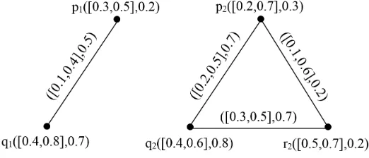
Example 4.3. Consider two EC-graphsM1=hα1, β1iandM2=hα2, β2ias shown in figure14.
Figure 14. EC-graphsM1 andM2
Then, their correspondingP-unionM1∪P M2 is shown in figure15.
Figure 15. P-union of EC-graphsM1and M2
Figure 16. R-union of EC-graphsM1andM2
It is easy to see that the cubic graphM1∪P M2 andM1∪RM2are neither EC-graph nor IC-graph.
We provide a condition for theP-union of two EC-graphs to be an EC-graph.
Theorem 4.3. LetM1=hα1, β1iandM2=hα2, β2ibe two EC-graphs such that
min
max{$+ α1(p), $
− α2(p)},
max{$− α1(p), $
+ α2(p)}
> max{µα1(p), µα2(p)}
≥ max
min{$+ α1(p), $
− α2(p)},
min{$− α1(p), $
+ α2(p)}
and min
max{$+β
1(e), $
− β2(e)},
max{$+ β1(e), $
− β2(e)}
> max{µβ1(e), µβ2(e)}
≥ max
min{$+β
1(e), $
− β2(e)},
min{$+β
1(e), $
− β2(e)}
for allp∈P ande∈Q.Then theP-union of two EC-graphs is an EC-graph.
We provide a condition for theR-union of two EC-graphs to be an EC-graph.
Theorem 4.4. LetM1=hα1, β1iandM2=hα2, β2ibe two EC-graphs such that
min
max{$+ α1(p), $
− α2(p)},
max{$− α1(p), $
+ α2(p)}
> min{µα1(p), µα2(p)}
≥ max
min{$+ α1(p), $
− α2(p)},
min{$− α1(p), $
+ α2(p)}
and
min
max{$+β
1(e), $
− β2(e)},
max{$+ β1(e), $
− β2(e)}
> min{µβ1(e), µβ2(e)}
≥ max
min{$+β
1(e), $
− β2(e)},
min{$+ β1(e), $
− β2(e)}
for allp∈P ande∈Q.Then theR-union of two EC-graphs is an EC-graph.
Theorem 4.5. Let M =hα, βibe a cubic graph which is not an EC-graph.Then there exist pi ∈P and
ei∈Qsuch that
µα(pi)∈($α−(pi), $+α(pi)) and µβ(ei)∈($−β(ei), $β+(ei)).
Proof. Straightforward.
Theorem 4.6. LetM =hα, βibe a cubic graph of Ω∗.IfM =hα, βiis both an IC-graph and an EC-graph,
then
µα(pi)∈U($eα)∪L($eα)
and
µβ(ei)∈U($eβ)∪L($eβ)
for allpi∈P andei∈Q⊆P×P.Where
U($eα) ={$+α(pi)|pi∈P}, L($eα) ={$
−
α(pi)|pi∈P}
and
U($eβ) ={$+β(ei)|ei∈Q}, L($eβ) ={$−β(ei)|ei∈Q}.
Proof. Assume thatM =hα, βiis both an IC-graph and an EC-graph. Then by definition we have
µα(pi)∈[$−α(pi), $+α(pi)], µβ(ei)∈[$β−(ei), $β+(ei)]
and
µα(pi)∈/($α−(pi), $+α(pi)), µβ(ei)∈/ ($−β(ei), $+β(ei)).
Thus µα(pi) = $−α(pi) or µα(pi) = $α+(pi) and µβ(ei) = $β−(ei) or µβ(ei) = $β+(ei). Hence µα(pi) ∈ U($eα)∪L($eα) andµβ(ei)∈U($eβ)∪L($eβ) for all pi ∈P andei∈Q⊆P×P.
Consider two cubic graphsM1=hα1, β1iandM2=hα2, β2iin Ω∗.If we exchangeµα1 byµα2 andµβ1 by
µβ2 we get the cubic graph as Mc1=
D
c α1,cβ1
E
andMc2=
D
c α2,cβ2
E
,respectively.
Example 4.4. Consider two IC-graphsM1=hα1, β1iandM2=hα2, β2ias shown in figure17.
Figure 17. IC-graphsM1 andM2
Then, their correspondingMc1 andMc2 are shown in figure18.
Figure 18. Cubic graphsMc1 andMc2
It is easy to see that the cubic graphsMc1 andMc2 are neither IC-graph nor EC-graph. Similarly, we can provide and example for two EC-graphs that are neither IC-graph nor EC-graph.
5. Application
Fuzzy graph theory is a platform which has wide range of applications in mathematics, computer science
etc. Cubic graph is a more general approach, which can be used in decision making very effectively.
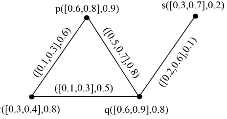
Suppose we have a set of three countries like,P ={X,Y,Z}as a vertex set and the membership of each
member of the set denotes the strength of that country over the neighbouring country with respect to future
and present time by considering its economic strength. Now we want to observe the effect of strength of one
certain information and data with respect to economy
α=
hX : [0.6,0.8],0.9i
hY : [0.5,0.9],0.7i
hZ : [0.3,0.7],0.8i
where interval membership predicts the economy of a certain country for the future and the other membership
shows economy of a certain country for the present time based on certain information and data with respect
to economy. Now on the basis ofα,we have the setβ of edges as follows
β =
hXY : [0.5,0.8],0.9i
hY Z: [0.3,0.7],0.8i
hZX: [0.3,0.7],0.9i
where interval membership predicts the effect of economy of a certain country for the future and the other
membership shows the effect of economy of a certain country for the present time at the other country. The
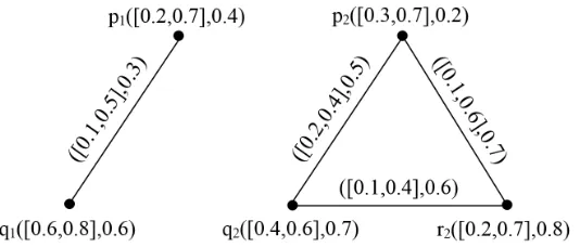
corresponding cubic graph is shown in figure19.
Figure 19. Cubic graph
So finally we concluded that economy of a certain country effect very much on the economy of the
neighboring countries.
6. Conclusions
Graphs are among the most ubiquitous models of both natural and human-made structures. They can
be used to model many types of relations and process dynamics in computer science, physical, biological
and social systems. We come up here with the idea of cubic graphs and we define different operations of
cubic graphs. We also provide a short application of cubic graph. In future we are planning to generalize
References
[1] M. Akram and W.A. Dudek, Interval-valued fuzzy graphs, Comput. Math. Appl., 61(2) (2011) 289-299. [2] M. Akram, Interval-valued fuzzy line graphs, Neural Comput. Appl., 21 (2012) 145-150.
[3] M. Akram and B. Davvaz, Strong intuitionistic fuzzy graphs, Filomat, 26(1) (2012) 177-196 [4] M. Akram, Bipolar fuzzy graphs, Inf. Sci., 181 (2011) 5548-5564.
[5] M. Akram, Bipolar fuzzy graphs with applications, Knowl.based Syst., 39 (2013) 1-8. [6] P. Bhattacharya, Some remarks on fuzzy graphs, Pattern Recognition Lett., 6 (1987) 297-302.
[7] R.A. Borzooei and H. Rashmanlou, Cayley interval-valued fuzzy threshold graphs, U.P.B. Sci. Bull., Ser. A, 78(3) (2016) 83-94.
[8] F. Buckley, Self-centered graphs, Ann. N.Y. Acad. Sci., 576 (1989) 71-78.
[9] Y.B. Jun, C.S. Kim and M.S. Kang, Cubic subalgebras and ideals of BCK/BCI-algebras, Far East J. Math. Sci., 44 (2010) 239-250.
[10] Y.B. Jun, K.J. Lee and M.S. Kang, Cubic structures applied to ideals of BCI-algebras, Comput. Math. Appl., 62(9) (2011) 3334-3342.
[11] Y.B. Jun, G. Muhiuddin, M.A. Ozt¨urk and E.H. Roh, Cubic soft ideals in BCK/BCI-algebras, J. Comput. Anal. Appl., 22(5) (2017) 929-940.
[12] Y.B. Jun, C.S. Kim and K.O. Yang, Cubic sets, Ann. Fuzzy Math. Inf., 4(1) (2012) 83-98.
[13] J.G. Kang and C.S. Kim, Mappings of cubic sets, Commun. Korean Math. Soc., 31(3) (2016) 423-431. [14] A. Kauffman, Introduction a la Theorie des Sous-emsembles Flous, Masson et Cie, 1 (1973).
[15] M. Khan, Y.B. Jun, M. Gulistan, N. Yaqoob, The generalized version of Jun’s cubic sets in semigroups, J. Intell. Fuzzy Syst., 28(2) (2015) 947-960.
[16] S.N. Mishra, H. Rashmanlou and A. Pal, Coherent category of interval-valued intuitionistic fuzzy graphs, J. Mult.-Val. Log. Soft Comput., 29(3-4) (2017) 355-372.
[17] J.N. Mordeson and P.S. Nair, Fuzzy graphs and fuzzy hypergraphs, Physica Verlag, Heidelberg (2001).
[18] G. Muhiuddin, S.S. Ahn, C.S. Kim and Y.B. Jun, Stable cubic sets, J. Comput. Anal. Appl., 23(5) (2017) 802-819. [19] M. Pal, S. Samanta and H. Rashmanlou, Some results on interval-valued fuzzy graphs, Int. J. Comput. Sci. Electr. Eng.,
3(3) (2015) 2320-4028.
[20] R. Parvathi, M. G. Karunambigai and K. Atanassov, Operations on intuitionistic fuzzy graphs, Proc. IEEE Int. Conf. Fuzzy Syst., (2009) 1396-1401.
[21] T. Pramanik, M. Pal and S. Mondal, Interval-valued fuzzy threshold graph, Pac. Sci. Rev. A: Nat. Sci. Eng., 18(1) (2016) 66-71.
[22] T. Pramanik, S. Samanta and M. Pal, Interval-valued fuzzy planar graphs, International J. Mach. Learn. Cybern., 7(4) (2016) 653-664.
[23] A. Rosenfeld, Fuzzy graphs, Fuzzy sets and their applications, Academic Press, New York, (1975) 77-95.
[24] S. Sahoo and M. Pal, Product of intuitionistic fuzzy graphs and degree, J. Intell. Fuzzy Syst., 32(1) (2017) 1059-1067. [25] M.S. Sunitha and K. Sameena, Characterization of g-self centered fuzzy graphs, J. Fuzzy Math., 16 (2008) 787-791. [26] S. Vijayabalaji and S. Sivaramakrishnan, A cubic set theoretical approach to linear space, Abstr. Appl. Anal., 2015 (2015)
Article ID 523129 8 pages.
![Figure 4. Cubic graph M1[M2]](https://thumb-us.123doks.com/thumbv2/123dok_us/8669235.1730294/6.612.208.406.78.186/figure-cubic-graph-m-m.webp)