DEVELOPMENT OF CONGESTION CAUSAL PIE CHARTS FOR
ARTERIAL ROADWAYS
Ali Soltani-Sobh1, Marija Ostojic2, Aleksandar Stevanovic3, Jiaqi Ma4, David K. Hale5
1 Department of Transportation City of Miami Beach, FL, USA 2 Northwestern University, Evanston, IL, USA
3 Department of Civil, Environmental, and Geomatics Engineering, Florida Atlantic University, FL, USA 4,5 Transportation Solutions Division, Leidos, Inc., VA, USA
Received 30 August 2016; accepted 7 February 2017
Abstract:Urban congestion is being increased by a rapid growth in travel demand and a limited ability to expand physical infrastructure. If transportation agencies could accurately quantify the impacts of various congestion causes, they would be able to prioritize their strategies more efficiently. The Federal Highway Administration developed a well-known congestion causal pie chart in 2004, but this development process did not have extensive access to field data. Recent advancements in both traffic measurement technologies and data-driven analysis are making it possible to quantify congestion impacts more accurately. However, an assessment of congestion causes on signalized arterials presents many challenges, due to complexity of the required data and the interaction of traffic demand and control. The objective of this study is to create congestion pie charts which demonstrate the proportion of average experienced delay components on arterial corridors. A multivariate linear regression model of observed delay is used to demonstrate contributing factors to arterial street congestion. The methodology is explained using a section of Broward Boulevard in Fort Lauderdale, FL. The findings from the model demonstrate that a considerable part of arterial congestion can be attributed to travel demands and intersection signals.
Keywords: congestion, arterial roadways, delay, signal timing, travel demand management.
1 Corresponding author: asoltanisobh@fau.edu 1. Introduction
Let us take, for example, a hypothetical situation in which a person travels home from a late-night meeting. He/she is taking his/her regular route through a heavily used arterial street. With the entire major street signals resting in the green phase, and very light traffic, he/she passes through the arterial in almost no time. We say this person experienced the free-flow travel time. On the next day, this same commute takes much more time due to heavy traffic, but
no irregular conditions. On the day after tomorrow, he/she experiences delays in the same PM peak due to an incident or work zone, and again on the following day because of heavy rain or snow/slush. The story continues every day by experiencing delay with and without presence of irregular causes.
congestion during these commute times. The most intuitive answer would be many other vehicles want to travel at the same time on the same road. However, it is certain that some nonrecurring factors such as inclement weather, traffic incidents, or work zones can significantly increase our travel times. On the other hand, some control measures such as traffic signals can add to the delay. They are there to produce safe movements through intersections and to serve as many vehicles as possible, but both of these goals may conflict with our objective to go through a corridor in the shortest possible time. Finally, traffic demand itself can be a nuisance (e.g. traffic causing difficulty with changing lanes) or major impedance (traffic from the downstream segment has spilled back to our link and we cannot move). How much does each of these factors contribute to our experienced delay on a daily basis? We cannot easily answer this question.
Even though a number of studies quantified most major causes of travel delay on freeways, no comprehensive attempts were found for quantifying arterial congestion causes. The objective of the study is to find out how much each of these factors contributes to the average commuting delay on arterial streets. The methodology is based on the linear regression to model observed delay as a function of various recurring and nonrecurring factors. The contribution of each factor is based on impact magnitude and the statistical frequency of factor occurrence. Impact magnitude is derived from the regression model, and the frequency of occurrence is estimated by averaging the value of the factor over the entire data set. Such identification provides quantitative insight into the cause of delay in the given arterial corridor as a pie chart and provides
guidelines to congestion mitigate strategies. For example, suppose the method results indicate that for the arterial corridor, 50% of delay is due to traffic demand, 10% is due to suboptimal signal timing, 20% is due to work zone, and the remaining 20% is due to incident. In such an example, it could be said that if retiming signals were operative under their optimum plan, a 10% reduction in average experienced delay would occur. The methodology to quantify contributions of individual congestion causes is applied on a well-ITS-equipped, signalized arterial in Central Broward, FL. The research presented here is based on a significant amount of ITS data from various detection devices (e.g. mid-block detectors and Bluetooth travel-time readers) and four months of event logs collected and reduced by Traffic Management Center staff.
2. Literature Review
period. (Chow et al., 2014) conducted an empirical study of urban traffic congestion in Central London, using an automatic plate number recognition system. The study proposed to interpret congestion and its causes through a linear regression model. The results suggested that 15% of congestion was caused by accidents, road work, and special events.
Building on their previous research, (Kwon et al., 2011) proposed a freeway corridor-level approach to attribute travel time variability to different causes: incidents, weather, work zones, special events and inadequate capacity. Similarly, (Hasan et al., 2011) presented a travel time variations prediction model based on individual vehicle speeds retrieved from multiple sources. The model-related travel time variability was attributed to vehicle type, traffic density and traffic composition, based on a nonlinear-latent-variable regression model. However, researchers admittedly neglected the presence of signals and turning movements due to data sources’ limitations. (Alvarez and Hadi, 2012) studied the metrics of reliability and indicated that travel time distributions vary among periods due to congestion, traffic f low and incidents. Furthermore, (Taylor and Somenhalli, 2014) estimated day-to-day travel time variability using Burr distribution properties and the Burr regression technique. Urban arterial travel time variability in Adelaide was modeled by considering traffic variables such as link length, congestion index and degree of saturation. (Hojati et al., 2016) developed a travel time reliability measure to calculate the extra travel time caused by traffic incidents. They found that each incident type’s EBT behavior followed specific patterns based on characteristics of the incidents.
(Anbaroglu et al., 2014) designed a non-recurrent congestion events detection methodology to accurately account for large urban corridor non-recurrent congestion. The authors developed a Link Journey Time measure, concluding that those at least 40% higher than expected were probably caused by non-recurring events. (Agarwal et al., 2005) used detector occupancy information, weather data, and pavement surface conditions to estimate capacity and speed decreases, due to varying intensities of rain and snow. (Chin et al., 2004) addressed the impact of inclement weather on freeway congestion, and concluded that light rain or snow, heavy rain and heavy snow reduce traffic speed by 10%, 16%, and 40%, respectively. (Goodwin, 2002) presented a literature review about weather effects on traffic flow on arterial roadways. The research concluded that traffic volume demands and flow rates are reduced by 6% to 30% during adverse weather conditions.
3. Arterial Congestion
Congestion on arterial (signalized) streets can be caused by various factors. Unlike on freeways (where congestion is mainly a result of high traffic demand (V/C > 1), work zones, incidents, special events and inclement weather) congestion on signalized roads can be also caused by signal timing and interaction with access points. Understanding the causes of observed congestion is the first important step to deploying an appropriate transport strategy to improve arterial road traffic. In this study, the goal is to develop a regression-based method to decompose observed congestion into different causes.
In order to examine the different components of congestion, an indicator to quantify the degree of congestion is needed. In this study, delay was used as the measure of congestion. Delay can be defined as actual travel time minus flow travel time. Generally, free-flow travel time is presented as the minimum time required for a vehicle to traverse a roadway. Some studies calculate free-flow travel time as a function of length and speed limit (Palacharla and Nelson, 1999; Lin et al., 2004). In this study, free-flow travel time is estimated based on the corresponding segment lengths and a ‘free flow speed’ classified as the speed limit.
Arterial Traffic Data
Fig. 1 shows the arterial road as a part of Broward Boulevard in Fort Lauderdale, FL. This corridor is approximately 3.6 miles long, and represents a major east/west connection from SR-7 (US-441) to Andrew Avenue. In this study, only the main street is considered without consideration of the turns and minor movements, due to the lack of information
and data on other movements. This road consists of five continuous segments separated by MVDS (Microwave Vehicle Detection System) mid-block detectors to collect volume data.
The collected data along this corridor is associated with each segment separately. Travel time data in this corridor is collected by Bluetooth devices. Bluetooth-based travel time measurement involves identifying and matching the Median Access Control (MAC) address of Bluetooth-enabled devices carried by motorists as they pass a detector location (Malinovskiy et al., 2010). The travel times of vehicles between two detectors are estimated by matching the MAC address. The travel times are processed and stored in 15-minute averages.
This study covers a set of data from September-December of 2014. Fig. 1 presents the average travel time and free-flow travel time (FFT) associated with each segment along the corridor in both E-W and W-E directions. The relative variations of average travel time with respect to FFT at various times of day are different in each segment. In some segments and times of day, the drivers travel at average speed lower than speed limit, which can be an indication of congestion and congestion contributing factors.
3.2. Congestion Measure - Delay
In general, factors contributing to arterial congestion can be categorized as recurrent and non-recurrent factors (Hasan et al., 2011). Recurrent congestion refers to congestion that commuters experience on a regular basis. In this study, recurrent congestion causes include travel demand, control congestion and access points. The control delay is the component of congestion that results from the type of control at the intersection. In this study, the control delay is separated into delay due to signals existence and delay due to the suboptimal signal timing plan. Causes of non-recurrent congestion include closures due to roadwork, traffic incidents, and adverse weather.
The methodology applies to a continuous arterial corridor divided into n segments which are equipped with Bluetooth devices and MVDS (Microwave Vehicle Detection System) mid-block detectors indexed i=1,…, n. Volume and travel time were measured and averaged for every 15-min interval indexed t=1, …, T. At segment i at time period t, delay was defined as travel time minus free-flow travel time. Travel time at segment i at time period t is the average travel time of all collected Bluetooth data at the corresponding segment and time period. Noted, the authors are aware of the bimodal value of travel time on arterial roads; essentially in correlation with making the green wave and missing the green wave. This value was indirectly considered in this study by using average travel time at segment i at time period t.
Considering the delay definition, in this study the goal is to answer how much each factor contributes to average experienced
delay. The delay at segment i at time t is defined as Eq.(1), Eq.(2):
(1)
(2)
where: D(i,t): Delay in segment i at time period t (second), TT(i,t): Average travel time in segment i at time period t (second), FFT(i): Free flow travel time in segment i (second), l(i): Length of segment i (mile), v(i): Speed limit in segment i (mph).
Fig. 2.
Arterial Road Case Study in Fort Lauderdale, and Average Experienced Travel Time in Each Segment
3.3. Causes of Congestion
The method of this study attempts to attribute delay as the measure of congestion to different components. The considered factors in this study and their data sources are explained as below for both case studies.
3.3.1. Travel Demand
Travel demand is the number of desired trips over a given road segment, and represents a major contributor to congestion. Road traffic volume is a widely-used indicator of travel demand. Actual weekday traffic demand was available from 5 MVDS mid-block traffic count detectors on each segment. In this study, vehicle miles traveled (VMT) was considered as a proxy of demand. Vehicle Miles Traveled (VMT) is one of the most common measures in estimating travel demand in the United States and has historically been used to determine the need for new infrastructure (Soltani-Sobh et al.,
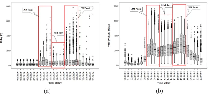
2016). For a given time period, VMT was estimated based on traffic volume counts and segment lengths. VMT was used to represent the effect of both traffic volume and traveling distance. Fig. 4 presents the hourly variation of travel demand collected from MVDS collectors. From the patterns of delay and travel demand, it can be extracted that the travel demand and delay are strongly correlated.
3.3.2. Signal Existence
delay due to traffic signals is quantified by comparing actual travel times during very low traffic demand (e.g. nighttime) with free-flow travel times. This definition is based on the fact that in night time when there is no non-recurrent factor and the traffic volume is low, the additional travel time over free flow travel time is contributed by signals at intersections. In this study, control delay is decomposed into signal existence and suboptimal signal timing. After suboptimal signal timing delay estimation, delay due to the signal existence can be estimated as control delay minus suboptimal signal timing delay.
3.3.3. Suboptimal Signal Timing
In this study, suboptimal signal timing was considered part of control delay. It demonstrates how much of the experienced delay in arterial traffic is contributed by not updated signal timing. The suboptimal signal timing variable is defined as the difference in intersection delay between existing (i.e. current) and optimized signal timing plans. The “current” state was introduced as the effectiveness of existing signal timing plans to serve current traffic demands. The “optimal” state represented effectiveness of updated signal timing plans in serving current traffic demands. This difference could be interpreted as a benefit of updating signal timing plans to better accommodate recent evolutions in traffic demand. It was expected that optimized signal timing plans would produce better performance (lower delay).
The Broward County Traffic Engineering Department conducted the most recent
retiming of signal timing plans in 2011 by developing several Synchro models. After this retiming effort, there were no further volume or timing adjustments to the Synchro files, but timing plans were fine-tuned in the field. In order to find out the delay of current and optimal signal timing plans, it was necessary to obtain current turning movement counts. Due to the availability of old traffic counts, old arterial traffic flow, and current arterial traffic flow from MVDS detectors, the current turning movement counts were estimated by growing the old turning movement counts by the growth factor of arterial traffic flow.
These updated turning movement counts were inserted into the appropriate Synchro file. These Synchro files were created for each time-of-day (TOD) in all weekdays over the study period. Each time of day period included two associated Synchro files, namely “current” and “optimized”. In the current scenario, the turning movement counts and signal timing plans are current, while in optimized scenario the signal timing plans are optimized based on current turning movement counts.
(a) (b) Fig. 3.
Hourly Variations of (a) Delay, (b) VMT over 24-hours
In each direction, performance of signal timing plans was assessed by quantifying the approach delay of intersections in each segment. The number of intersections in each segment is different. The signal performances also vary over time due to the variations in traffic volume. That means the signal performance are estimated for each times of day (AM, Mid-day, and PM) every day within period of study. The difference in delay resulted from Synchro was used as the measure of signal timing plan performance Eq.(3):
(3)
where: SST(i,t): Measure of Suboptimal Signal Timing of intersection i at time interval t, CSDn(i,t): Intersection (n) signal
delay at segment i at time period t (current signal plan), OSDn(i,t): Intersection (n)
signal delay at segment i at time period t (optimum signal plan).
3.3.4. Work Zones and Incidents
Event logs provide information related to work zones and traffic accident. An event log retrieved from the Broward County Transportation Management Center (TMC) provided information per type of event, start time (time it was logged), location (if it spread over several segments or impacted only one), number of lane closures, and end time (when the event was cleared). The traffic incident and work zone variables are both binary.
3.3.5. Weather
The value of precipitation (in inches) was used as the measure of adverse weather. A web application/software was used to provide relevant precipitation data during the studied time frame. Depending on the actual zip code information, specific area limits along the entire corridor were determined. More than one zip code signified potentially different weather conditions at different areas during the same time period.
3.3.6. Number of Access Points
In addition to signalized intersections, driveways, openings in the right-hand side of roadway, and median openings are expected to influence traffic flow. A large number of access points can increase potential conflicts. Fewer access points spaced farther apart allow for more orderly merging of traffic, and lesser delay. Access points do not have any information about demand and they are just indicating disturbances on main traffic.
4. Regression Based Decomposition
Model
There have been extensive bodies of researches on application of various mathematical, statistical, and econometric models in science and engineering (e.g. Asgari et al., 2015; Ahmadi and Merkley, 2009; Baratian-Ghorghi and Zhou, 2015). A linear regression model was developed to decompose the observed delay into various factors. The linear model was chosen based on the assumption that each of the explanatory variables contributes linearly to the delay. (Chow et al., 2014) and (Kwon et al., 2006) suggest linear regression decomposes delay in urban area and freeway. A more complex relationship could exist between variables,
but it is not considered in this study to keep the number of model parameters small, (e.g. adverse weather and number of incident). However, if enough data is available and the interaction is strong enough, such interaction terms could be considered. For our case study data in Fort Lauderdale, the weather coefficient correlation with incidents is only 0.049, which is negligible. The linear regression model in which delay observed at segment i, and time interval t, D(i,t) was defined as follows, Eq. (4), Eq.(5):
(4)
(5)
where: β0: value of intercept of the regression
model, β: vector of the model parameters for the associated explanatory variables, VMT(i,t): vehicle miles traveled (volume × segment length) at segment i and time interval t, Signal(i,t): signal existence measure at segment i and time interval t, SST(i,t) : suboptimal signal timing measure at segment i and time interval t, Weather(i,t) : precipitation measured at segment i and time interval t, WZ(i,t) : 0-1 indicator equal to 1 for an active work zone at segment i and time interval t, TI(i,t) : 0-1 indicator equal to 1 for a traffic incident at segment i and time interval t, A(i) : the number of access points along segment I, ϵ(i,t) : error term following the normal distribution with a mean of zero, and a finite variance.
coefficients, the model was fitted to data via the linear least-squares method. One statistical specification used in the model estimation procedure is transforming dependent var iable data. Nor ma l ly distributed of residuals is a pre-requisite for linear regression analysis. In this study, the residuals of dependent variable (delay) were often not normally distributed. However, an appropriate transformation was applied to yield data set residuals following approximately a normal distribution. The
applied data transformation was (i.e., delay was transformed to delay0.5). In
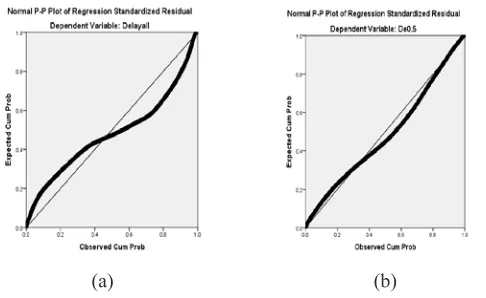
order to test data normality of residuals, the P-P plot of regression standardized residual was used. The P-P plot depicts observed cumulative probability values versus expected normal values of a given variable. P-P plots (before and after the delay transformation) are presented in Fig. 5. The criterion for normal distribution of residuals is the degree to which the plot coincides with reference line.
(a) (b) Fig. 5.
P-P Plot, (a) Original Delay, (b) After Transformation
4.1. Regression Results
It was mentioned that model parameters were estimated using the least-squares method. Results of regression over more than 30000 data points related to various 15-minute time intervals and road segments are summarized in Table 1. As noted, the dependent variable was Delay0.5, thus estimation of pie charts
and interpretation of results are based on transformed case. Applying the square-root function can be justified based on the facts that delay is known to grow non-linearly with increasing traffic intensity, generally
with a power of 2. The validity of the fitted model was tested using the F-statistic with practically zero p-value for all four models. The linear regression model successfully explains the delay variation. The last column of results shows adjusted R2 values,
from zero. The t-value is estimated as the ratio of the parameter’s coefficient to the associated standard error. The p-value confirms the probability that the true value of that parameter is different from zero.
From Table 1, the following are observed:
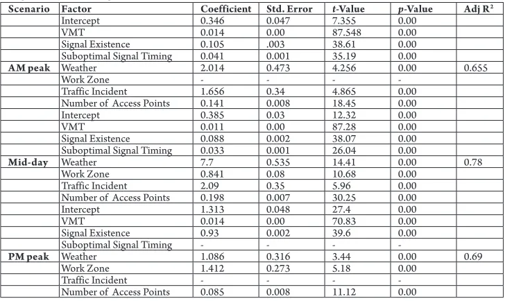
• The R-square is more than 60% for all the scenarios, and shows more than 60% of delay variation is due to the variation of the selected contributing factors. Based on dependency of delay to travel time, it can also be concluded that more than 60% of travel time variability can be defined by these factors variation. • Estimated coefficients demonstrate that
all the explanatory variables have proper sign, since positive sign indicates that the factors are contributing to the delay. Note that variables with p-value >0.05 were treated insignificantly and removed from the model regardless of sign.
• Intercept, Demand, Signal existence, Work zone, and Access points all are significant variables for the observed delay in all scenarios. These factors are associated with a p-value <0.001. • From t he rec u r rent v a r i able s ,
Suboptimal signal timing is not significant in PM peak scenarios. The insignificant suboptimal signal timing demonstrates the retiming the signals do not have effect on mitigating the delay in PM peak period.
• The number of access points is a delay-increasing factor. Because the data set is a combination of various segments with different numbers of access points, the results imply that segments having more access points induce more delay. The effect of access points on delay in the Mid-day scenario is higher than the other scenarios, likely because the frequency of commutes during the AM and PM periods compared with Mid-day.
Table 1
Congestion Causal Regression Model Results
Scenario Factor Coefficient Std. Error t-Value p-Value Adj R2
Intercept 0.346 0.047 7.355 0.00
VMT 0.014 0.00 87.548 0.00
Signal Existence 0.105 .003 38.61 0.00
Suboptimal Signal Timing 0.041 0.001 35.19 0.00
AM peak Weather 2.014 0.473 4.256 0.00 0.655
Work Zone - - -
-Traffic Incident 1.656 0.34 4.865 0.00
Number of Access Points 0.141 0.008 18.45 0.00
Intercept 0.385 0.03 12.32 0.00
VMT 0.011 0.00 87.28 0.00
Signal Existence 0.088 0.002 38.07 0.00
Suboptimal Signal Timing 0.033 0.001 26.04 0.00
Mid-day Weather 7.7 0.535 14.41 0.00 0.78
Work Zone 0.841 0.08 10.68 0.00
Traffic Incident 2.09 0.35 5.96 0.00
Number of Access Points 0.198 0.007 30.25 0.00
Intercept 1.313 0.048 27.4 0.00
VMT 0.014 0.00 70.83 0.00
Signal Existence 0.93 0.002 39.6 0.00
Suboptimal Signal Timing - - -
-PM peak Weather 1.086 0.316 3.44 0.00 0.69
Work Zone 1.412 0.273 5.18 0.00
Traffic Incident - - -
5. Congestion Pie Development
Based on data availability at various segments, delay is constituted in this study by seven components, Eq. (6):
(6)
In all pie charts, portion of each contributing factor is due to magnitude of effects and frequency of factor. The delay components in pie charts are affected by the coefficient estimation (magnitude) and the average value of variables (frequency). Given the
estimated coefficient from regression model and average value of different variables over all sample point data (all segments i and all time intervals t), the components of delay can be estimated for the entire corridor over study period as the following Eqs. (7-14):
average delay caused by demand (7)
average delay caused by signal existence (8) average delay caused by suboptimal signal timing (9) average delay caused by weather (10) average delay caused by work zones (11) average delay caused by traffic incidents (12) average delay caused by access points (13)
(14)
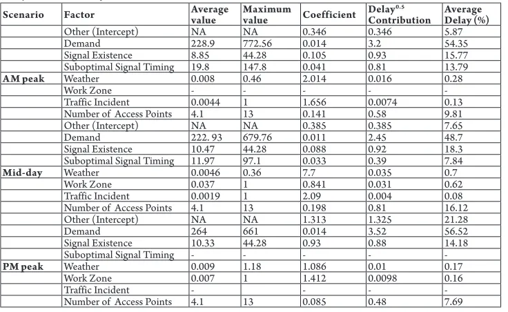
Table 2 presents the estimates of the delay components using the method presented in equation (7-14). Note that the model coefficient is regressed on square-root of delay; therefore, the portion of each contributing factor (percentage) is based on regressed square-root of delay.
These pie charts investigate how much each of these factors contributes to average experienced commuting delay. As an example, it can be interpreted that based on the collected data on arterial case study, in AM period, 54.35% of the average delay over period of study is caused by VMT, 15.77%
is due to signal existence, 13.79% is based on suboptimal signal timing, etc.
The presented pie charts in Fig. 6 imply that most arterial congestion regardless of scenario is caused by travel demands. One-half of the delay is due to the travel demand, which means delay can be considerably reduced by demand management and modifying trip patterns.
control delay. Given that signal timing plans change between time periods, the suboptimal signal timing might have different impacts in the different time periods. Experienced delays caused by suboptimal signal timing were 14% and 8% in the AM and Mid-day scenarios, respectively. This demonstrates that current signal timing plans, especially in Mid-day, is not optimally matched to demand. Suboptimal signal timing displayed no contribution to PM peak delay.
All of the pie charts show that a portion of delay is not easily explained by any variables. The impacts of those variables are denoted as “Other” in the pie charts. While there is no clear indication of what constitutes this category, it is possible that factors such as road geometry, transit operations, school zones, on-street parking, driver behavior, and imprecision of travel time measurements are contributing to the unexplained part of
congestion. To illustrate this speculation, it is widely known that Bluetooth travel-time-measurement devices error on the side of reporting higher travel times due to capturing more slow-moving vehicles. Therefore these devices sometimes report not only higher travel times, but also more delays, than true average values in the field.
6. No rmalized C ongestion Pie
Development
Based on the results of developed models in Table 1, almost all of the factors affect delay significantly. This means their variations statistically affect delay variations, and if any of these factors occurs, delay is changed significantly. However, the contributions of these factors to average delay are not considerable. It is because of the fact that frequencies of these events (over time at various segments) are relatively small.
Table 2
Delay Contributions from Various Causes
Scenario Factor Average value Maximum value Coefficient DelayContribution0.5 Average Delay (%)
Other (Intercept) NA NA 0.346 0.346 5.87
Demand 228.9 772.56 0.014 3.2 54.35
Signal Existence 8.85 44.28 0.105 0.93 15.77
Suboptimal Signal Timing 19.8 147.8 0.041 0.81 13.79
AM peak Weather 0.008 0.46 2.014 0.016 0.28
Work Zone - - - -
-Traffic Incident 0.0044 1 1.656 0.0074 0.13
Number of Access Points 4.1 13 0.141 0.58 9.81
Other (Intercept) NA NA 0.385 0.385 7.65
Demand 222. 93 679.76 0.011 2.45 48.7
Signal Existence 10.47 44.28 0.088 0.92 18.3
Suboptimal Signal Timing 11.97 97.1 0.033 0.39 7.84
Mid-day Weather 0.0046 0.36 7.7 0.035 0.7
Work Zone 0.037 1 0.841 0.031 0.62
Traffic Incident 0.0019 1 2.09 0.004 0.08
Number of Access Points 4.1 13 0.198 0.81 16.12
Other (Intercept) NA NA 1.313 1.325 21.28
Demand 264 661 0.014 3.52 56.52
Signal Existence 10.33 44.28 0.93 0.88 14.18
Suboptimal Signal Timing - - - -
-PM peak Weather 0.009 1.18 1.086 0.01 0.17
Work Zone 0.007 1 1.412 0.0098 0.16
Traffic Incident - - -
(a) (b)
(c)
Fig. 6.
Congestion Pie Charts (a) AM, (b) Mid-Day, and (c) PM
Fig. 6 indicates average contribution of these causes to delay, although it is not clear how average experienced delay will change due to variation of these factors. In order to demonstrate the relative effect of various factors on delay, a set of normalized pie charts were developed by considering each factor’s maximum value instead of using the average value. As presented in Fig. 7, the normalized pie charts disregard the effect of factors’ frequency, and demonstrate the magnitude of various factors’ effects on delay, and the changeability of average delay due to variation of the factors. For example; incident occurrence in the AM peak
increases the delay by 6.3% while increasing the rain by 100% induced 3.5% more delay. Based on these pie charts:
• Changing travel pattern to shift the AM and PM peak trips to other times of day is an effective strategy to decrease the delay. • Controlling the access point to the
arterial road can decrease delay considerably in Mid-day peak (12.55%). • Retiming intersections’ signals can be
more effective in AM peak by reducing 23.05% of average experienced delay. • Incident occurrence, induce more delay
(a) (b)
(c)
Fig. 7.
Normalized Congestion Pie Charts (a) AM, (b) Mid-Day, and (c) PM
7. Conclusions
The mitigation of traffic congestion can be facilitated by understanding the nature and causes of congestion. This study used a linear regression model to quantify individual congestion causes on arterial corridors. The objective of this study was to create congestion pie charts which demonstrate a proportion of delay components on arterial corridor. As a practical application, if agencies know congestion causes, they can strategize in order to mitigate congestion and the likely impact of such measures.
Mainly based on the availability (nature, access, coverage, etc.) of traffic data, a portion of Broward Boulevard in Fort Lauderdale, Florida was selected for an arterial road case study. The proposed methodology should be applicable to arterial
roads elsewhere with supply of relevant data. Average experienced delay was modeled as a function of travel demand, signal existence, suboptimal signal timing, number of access points, adverse weather, work zones, and traffic incidents. Suboptimal signal timing was defined as the intersection delay difference under existing and optimized signal timing plans. The optimum signal plan was designed by Synchro for 17 intersections, using the latest traffic volumes.
are too low to be presented as major delay factors in congestion pie charts over a longer period of time. As an example of pie charts interpretation for this case study over 4 months, in AM peak around 54% of average delay is due to the traffic demand, 16% is due to existence of signals, 14% is due to suboptimal signal timing, 10% is due to number of access points (too many ins and outs disturb the mainline traffic), 1% is due to adverse weather, and 5% is due to unknown factors (pedestrians, public transit, etc.).
Recurrent factors such as high demand, signal existence, suboptimal signal timings, and access point conflicts can produce corridor-wide congestion. Thus, to mitigate arterial congestion, transportation management agencies can prioritize their strategies to ref lect proportional importance of the causal congestions factors. Future research could include the use of more advanced statistical techniques such as panel data regression in order to take spatiotemporal details into account. In addition, signalized arterial corridors should be modeled through microscopic simulation software, to further investigate congestion causes under different scenarios.
References
Agarwal, M.; Maze, T.H.; Souleyrette, S. 2005. Impacts of weather on urban freeway traffic flow characteristics and facility capacity. In Proceedings of the 2005 mid-continent transportation research symposium, 18-19.
Ahmadi, L.; Merkley, G.P. 2009. Planning and management modeling for treated wastewater usage,
Irrigation and drainage systems 23(2-3): 97-107.
Alvarez, P.; Hadi, M. 2012. Time-variant travel time distributions and reliability metrics and their utility in reliability assessments, Transportation Research Record: Journal of the Transportation Research Board
2315: 81-88.
Anbaroglu, B.; Heydecker, B.; Cheng, T. 2014. Spatio-temporal clustering for non-recurrent traffic congestion detection on urban road networks, Transportation Research
Part C: Emerging Technologies 48(2014): 47-65.
Asgari, H.; Jin, X.; Mohseni, A. 2014. Choice, Frequency, and Engagement – A Framework for Telecommuting Behavior Analysis and Modeling, Transportation Research Record: Journal of the Transportation Research Board 2413: 101-109.
Baratian-Ghorghi, F.; Zhou, H. 2015. Investigating Women’s and Men’s Propensity to Use Traffic Information in a Developing Country, Transportation in Developing Economies 1(1): 11-19.
Chin, S.M.; Franzese, O.; Greene, D.L.; Hwang, H.L.; Gibson, R.C. 2004. Temporary losses of highway capacity
and impacts on performance: Phase 2. US - Department of
Energy. USA. 131 p.
Chow, A.H.F.; Santacreu, A.; Tsapakis, I.; Tanasaranond, G.; Cheng, T. 2014. Empirical assessment of urban traffic congestion, Journal of Advanced Transportation
48(8): 1000-1016.
Goodwin, L. C. 2002. Weather impacts on arterial traffic
flow, Available from internet: <https://ops.fhwa.dot.
gov>.
Kwon, J.; Barkley, T.; Hranac, R.; Petty, K.; Compin, N. 2011. Decomposition of travel time reliability into various sources: incidents, weather, work zones, special events, and base capacity, Transportation Research Record: Journal of the Transportation Research Board 2229: 28-33. Kwon, J.; Mauch, M.; Varaiya, P. 2006. Components of congestion: Delay from incidents, special events, lane closures, weather, potential ramp metering gain, and excess demand, Transportation Research Record: Journal of the Transportation Research Board 1959: 84-91. Lin, W.H.; Kulkarni, A.; Mirchandani, P. 2004. Short-Term Arterial Travel Time Prediction for Advanced Traveler Information Systems, Journal of Intelligent Transportation Systems: Technology, Planning, and Operations
8(3): 143-154.
Malinovskiy, Y.; Wu, Y.J.; Wang, Y.; Lee, U.K. 2010. Field experiments on bluetooth-based travel time data collection. In Proceeding of the Transportation Research Board 89th Annual Meetingm, No. 10-3134.
Palacharla, P.V.; Nelson, P.C. 1999. Application of Fuzzy Logic and Neural Networks for Dynamic Travel Time Estimation, International Transactions in Operational
Research 6(1): 145-160.
Skabardonis, A.; Varaiya, P.; Petty, K. 2003. Measuring recurrent and non-recurrent traffic congestion,
Transportation Research Record: Journal of the Transportation
Research Board 1856: 118-124.
Soltani-Sobh, A.; Heaslip, K.; Bosworth, R.; Barnes, R.; Song, Z. 2016. Do Natural Gas Vehicles Change Vehicle Miles Traveled (VMT)? An Aggregate Time Series Analysis, In Proceeding of the Transportation Research Board 95th Annual Meeting,No. 16-0192.
Hojati, A.T.; Ferreira, L.; Washington, S.; Charles, P.; Shobeirinejad, A. 2016. Modelling the impact of traffic incidents on travel time reliability, Transportation Research Part C: Emerging Technologies, 65: 49-60.
Taylor, M.A.P.; Somenahalli, S. 2014. Urban Arterial Road Travel Time Variability Modeling Using Burr Regression. In Proceeding of the Transportation Research