Type of the Paper: Article
1
A GIS-based method for identification of wide area
2
rooftop suitability for minimum size PV systems
3
using LiDAR data and photogrammetry
4
Diane Palmer 1, *, Elena Koubli 1,2, Ian Cole 1,3, Ralph Gottschalg 4,5 and Thomas Betts 1
5
1 Centre for Renewable Energy Systems Technology (CREST), Loughborough University, LE11 3TU, UK;
6
7
2 SolarCentury, London
8
3 FOSS Research Centre for Sustainable Energy of the University of Cyprus (UCY); [email protected]
9
4 Fraunhofer Center for Silicon-Photovoltaic (CSP), 06120 Halle, Germany;
10
11
5 EMW, Hochschule Anhalt, 06366 Köthen, Germany
12
* Correspondence: [email protected]; Tel.: +44-1509-635604
13
14
Abstract: A new method for wide-area urban roof assessment of suitability for solar photovoltaics
15
is introduced and validated. Knowledge of roof geometry and physical features is essential for
16
evaluation of the impact of multiple rooftop solar photovoltaic (PV) system installations on local
17
electricity networks. This paper begins by reviewing and testing a range of existing techniques for
18
identifying roof characteristics. It was found that no current method is capable of delivering
19
accurate results with publicly available input data. Hence a different approach is developed, based
20
on slope and aspect using LIDAR data, building footprint data, GIS tools and aerial photographs. It
21
assesses each roof’s suitability for PV installation. That is, its properties should allow the
22
installation of at least a minimum size photovoltaic system. In this way the minimum potential
23
solar yield for region or city may be obtained. The accuracy of the new method is then established,
24
by ground-truthing against a database of 886 household systems. This is the largest validation of a
25
rooftop assessment method to date. The method is flexible with few prior assumptions. It is based
26
on separate consideration of buildings and can therefore generate data for various PV scenarios
27
and future analyses.
28
Keywords: solar; LiDAR; rooftop photovoltaics; building characteristics; wide-area solar yield.
29
30
1. Introduction
31
1.1 Significance of 3D rooftop attributes for photovoltaic system installation and yield
32
Precise estimation of the solar energy resource on pitched roofs is crucial for modelling
33
photovoltaic (PV) installation in residential scenarios. However, there is no national database of
34
building characteristics in the UK. This is also a common omission in other countries. The EU
35
Buildings Database [1] contains information on gross floor area and roof insulation type but has no
36
details of roof inclination, orientation or pitched dimensions. The US is slightly better provided for
37
with a report which assesses the rooftop solar PV potential of 23% of buildings nationwide [2]. In
38
this paper, previous work described in [3–5] is re-visited and expanded. That is, automated
39
extraction of building roof plane characteristics over wide areas, shading techniques and the
40
influence of module orientation on yield are studied. A grid square (pixel)-based approach to
41
estimation of solar energy potential over pitched roofs is developed. This is achieved by combining
42
publicly available building outline maps with aircraft-based LiDAR (Light Detection and Ranging)
43
data. These are analysed statistically within a Geographical Information Systems (GIS) environment.
44
The new approach is validated against data from a selection of approximately 2000 citywide PV
45
systems currently installed in Nottingham, UK. Up to the present, no other rooftop PV capacity
46
studies have been as rigorously validated.
47
1.2 PV in the built environment
48
There is strong growth of PV in the built environment. To date in the UK, rooftop PV has been
49
deployed faster than expected. 20% of total installed solar PV capacity (2.6 GW) comes from small
50
scale 0 to 4 kW installations [6]. Net-metering to encourage self-consumption is taking place in the
51
UAE, Lebanon, Chile and parts of India [7]. In the Netherlands household installations comprise
52
90% of PV capacity [8]. In China, rooftop distributed installations reached 15 GW in 2017, a rise of
53
400-500% compared to 2016 [9].
54
Modern living space offers a range of challenges and opportunities for solar panel installation.
55
Many neighbourhoods display complex amalgams of roof pitch (tilt) and building orientation
56
(azimuth). Roof features such as chimneys, vent pipes, aerials, roof lights, cross-gables, and dormers
57
may further reduce possible system size.
58
Roof pitch is linked to building age and roofing material. These in turn are related to
59
geographic regional variation in construction methods. Building orientation (azimuth) is largely
60
dictated by road layout which is a reflection of local topography.
61
1.3 The influence of tilt and azimuth on rooftop solar irradiation
62
The tilt and azimuth of a PV system have two main influences on energy yield. First, there is an
63
increase or decrease in annual total yield depending on how well the roof pitch and azimuth match
64
the average sun position over the year [10]. Second, the daily or seasonal timing of peak energy
65
generation is influenced [11].
66
Solar panels may capture the maximum solar radiation by inclination at an optimal angle
67
dependent on sun path (site latitude) and typical weather (diffuse fraction of solar radiation), which
68
is about 38 degrees for most of the UK. Roofs which have higher or lower pitches than this optimal
69
value receive less irradiation.
70
Existing housing stock does not always allow the use of this optimum and compromises in
71
deployment are necessary. Similar mismatches occur in other countries. Whereas the traditional UK
72
roof pitch (40-50⁰) [12] tends to be steeper than the optimum angle for PV, in Mediterranean regions
73
traditional tile roofs (20-25⁰) [13] are frequently shallower than the optimum 30-33⁰. Azimuth may
74
also be less than ideal. Although total annual yield is lowered by non-optimal building orientation
75
there may be positive side effects such as higher morning, evening and winter generation.
76
Analysis of roof characteristics and their impact on PV output and timing for an individual
77
house is relatively straightforward. This research provides an efficient method for analysing areas
78
too large to investigate manually.
79
1.4 Research Methodology in Brief
80
There has been substantial previous research into computerised recognition of
81
three-dimensional structural features. [14–16] provide excellent literature reviews. The authors of
82
[14] divide rooftop area estimation methods into three. First, the constant value methods approach
83
the problem collectively by scale-up e.g. [17]. Although quick and easy, they employ broad
84
assumptions and produce generalized results. Second, manual selection e.g. [18] which is
85
time-consuming. Third, GIS-based methods e.g. [3] which deliver detail and may be automated but
86
require substantial computing power. No technique is widely accepted as definitive. This paper
87
concentrates on GIS-based methods.
88
This area of research is challenging in terms of both data quality and the sheer size of LiDAR
89
datasets. Additionally, 3D feature extraction is non-trivial. First, existing methods using both LiDAR
90
and aerial photography as inputs are tested. The advantages and disadvantages of these techniques
91
voting, LiDAR edge detection, image edge detection, image recognition and hill shading with
93
ambient occlusion.
94
LiDAR datasets are a grid of height values from an aircraft flying at constant altitude pulsing a
95
laser to Earth and timing the returns. The number of returns per square metre determines the
96
resolution of the data. LiDAR supplies detailed heights of objects (e.g. buildings and vegetation), as
97
well as terrain surface. In the UK, LiDAR data is supplied by the Environment Agency [19]. Several
98
resolutions are available for limited areas. 1 m resolution was chosen as the best compromise
99
between accuracy and availability. It covers approximately 70% of England. Aerial photography was
100
obtained from GoogleEarth [20].
101
Since none of the existing methods was found to be adequate using the available input data, a
102
new approach is elaborated. This is expedient for medium resolution LiDAR. Previous methods may
103
result in imprecise values unless high resolution data is available. Rather than attempting to obtain
104
exact roof areas, each roof is assessed to discover whether it is suitable for PV installation. Suitability
105
here is defined as a roof to which at least a minimum size photovoltaic system may be fitted (8 m2 of
106
roof area corresponding to a 1 kW system, assuming a panel size of 1.6 m2 [14]), with an azimuth
107
East through South to West and tilt of between 15⁰ and 60⁰. (Most UK homeowners install a 1 kW to
108
4 kW solar panel system on their roof [21].) Thus, the minimum potential solar yield for region or
109
city may be obtained. The need to generate accurate roof areas and PV system sizes from inexact
110
data is avoided because the goal is the minimum requirements for domestic PV only. Nor is this
111
method intended to separately identify multiples of 1 kW. This is not possible with the available
112
input data and domestic systems are almost entirely comprised of smaller multiples e.g. 3.76 kW.
113
LiDAR heights on roof tops only are selected by clipping them out using building outlines
114
(from OS MasterMap Topography Layer [22]) as patterns or “cookie cutters”. The tilt and azimuth of
115
each roof pixel is calculated by weighted least squares fit of a plane to a 3 × 3 pixel neighbourhood,
116
centred on each LiDAR point (see [3] for details). Due to LiDAR inaccuracies, flight paths and
117
chance, this will result in a unique value for each pixel. Roofs slope evenly, so a statistical technique
118
smoothing azimuth pixel values into groups is identified. Next the roof is divided into separate
119
planes according to the grouping. The size, tilt and azimuth of each plane is known from the
120
calculation just carried out. A check is performed to ascertain whether a system of 8 m2 can be
121
mounted on any of the roof faces.
122
Two case studies are used to test the methods. The first is the Wollaton Park area of
123
Nottingham, UK. This was selected for the variety of architectural styles displayed by its houses. The
124
second is a set of about 2000 housing association domestic installations in Nottingham. Locations,
125
system sizes, and installer records of the tilt and azimuth of each of these systems have been
126
gathered from a monitoring portal.
127
2. Review and test of existing methods of rooftop PV estimation
128
2.1 Simple Roof slope and azimuth extraction
129
Trigonometry may be applied to the LiDAR grid of roof point heights to calculate tilt and
130
azimuth of every grid square or pixel (2 m, 1 m, 50 cm, 25 cm or 15 cm, depending on the resolution
131
available in the area of interest). The traditional approach is to group pixel values obtained from a 3
132
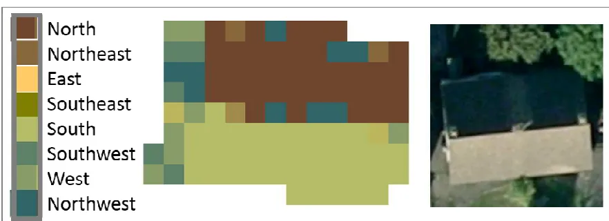
× 3 neighbourhood by compass point bands to produce realistic roof planes [23]. However, Figure 1
133
illustrates the problems which may occur. The building in the aerial photograph has a simple roof
134
layout, comprising one north and one south-facing roof section. (Note: the overhead perspective
135
images in this paper are of poor quality. This is a reflection of the data which is publicly available
136
and is part of the problem which this paper seeks to address.) Whilst the azimuth diagram generated
137
from LiDAR reproduces the two sections, there are many spurious small roof planes pointing in
138
various directions. These result from the presence of chimneys, TV aerials etc, as well as
139
overhanging trees and surrounding structures such as garages. In the case of more complex roof
140
142
Figure 1. Roof Azimuth produced from 1 m LiDAR compared to aerial photograph for a two-roof plane
143
building
144
145
Extraction of roof geometry from LiDAR has been the subject of extensive research over the last
146
ten years. Existing solutions are categorised, reviewed and tested in the following paragraphs.
147
2.2 Model Driven Methods
148
This approach comprises the matching of the irregular roof segment shapes obtained from
149
LiDAR to the best-fitting model in a library of basic building shapes. Jacques et al (2014) [24] utilise it
150
to classify small buildings in the city of Leeds, UK, using a restricted catalogue of common roof
151
profiles (gabled, hipped, flat, complex, or unclassified).
152
Model-based methods do not work well for multifaceted roof shapes and intricate building
153
construction. Looking at the topic from a country-wide perspective, there are numerous possible
154
building types. Internationally, roof type is just as varied [25]. Some authors list as many as 50
155
categories with multiple sub-categories. The Geograph Britain and Ireland Project [26], which
156
collects representative photographs for every square kilometre of the nation, has captured examples
157
of over 25 different roof profiles. Some have very different forms (e.g. flat, round or hipped dormer).
158
Due to the multiplicity of possible model shapes, this line of research was not pursued.
159
2.3 Histogram discrimination / peak detection
160
This approach is perhaps the oldest and simplest. Peaks are searched for in elevation (above
161
ground level), tilt or azimuth histograms and used to segment the data. Spatial planes are fitted for
162
each segment. Theoretically, simple gabled roofs should display a rectangular height histogram and
163
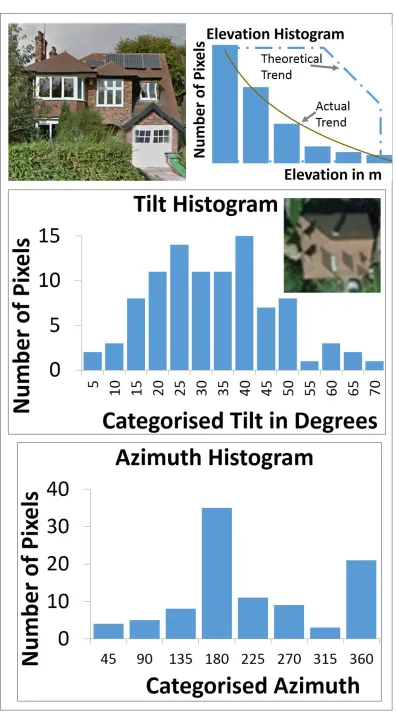
that of hip roofs should resemble a trapezium [27]. In fact, these ideals cannot be achieved with real
164
data, as Figure 2 explains. The Wollaton Park (Nottingham) house in the Figure 2 example is a
165
complex but not unusual structure, comprising a hipped roof with a porch and dormers. Its
166
elevation histogram should slope gently straight down (in the shape of a trapezium [27]) but in
167
reality is concave (see dotted and solid lines in Figure 2 top right). The building in question is known
168
to have a roof tilt of 38⁰ (the same for each of the two major front and rear planes). Actually, it is
169
barely possible to distinguish the 35-40 degree bin as the most frequently occurring in the tilt
170
histogram. (This is obvious on a simpler roof form.) The azimuth histogram is a little clearer in as far
171
as the major front (south-facing, 180⁰) and rear (north-facing, 360⁰) planes may be discerned. Then
172
174
Probably because of these kind of problems, the peak-fitting method seems to have been largely
176
replaced by other techniques. Furthermore, it analyses each height point in isolation. The spatial
177
relationship between points is not considered, although all the points on a plane will have related
178
values until an edge is reached. Newer methods refine peak detection with iterative voting (e.g.
179
region-growing [28], random sample consensus algorithm (RANSAC) [29] and Hough Transform)
180
[30]. These are all region dependent i.e. they account for the spatial location of each height point with
181
reference to its neighbour. The Hough Transform is the computationally fastest of these techniques.
182
Hough plane detection has two stages: edge detection, followed by grouping of the points
183
inside the edges to generate the planes.
184
2.4 Edge Detection
185
Initially, a Canny edge detector [31] was applied to the 1 m LiDAR data for the Nottingham
186
house in Figure 2 (GRASS software, i.edge [32]). The Canny edge detector is well known and often
187
used to process both LiDAR data and images. It works by marking local maxima in the LiDAR as
188
edges. However, in the case of the Nottingham building in Figure 2, the Canny algorithm completely
189
failed to discriminate any edges (roof ridges), due to noise and the relatively coarse resolution of the
190
data. When tested on several of the smaller housing association properties, edges were detected but
191
not all correctly (Figure 3). On some homes the roof ridge is identified but on others an edge
192
perpendicular to the expected position is located. With no clear or consistent pattern to these errors,
193
further algorithms were trialled with the aim of improving reliability.
194
195
196
Figure 3. Results of Canny Edge detector applied to identify roof ridges on small Nottingham homes
197
198
These included the simple (moving window) filter of SAGA GIS [33], and ArcGIS [34,35] low
199
pass (3 × 3 cell area mean), majority (3 × 3 cell area mode) and high pass (3 × 3 cell area weighted)
200
filters. There was no improvement in results. Roof ridges appeared too wide or were not detected.
201
The problem appears to be the resolution of the input LiDAR data. Roof features are too small
202
to be easily perceptible in 1 m data. Figure 4 illustrates the LiDAR data for the example
203
Nottingham house in the form of a simple graph. The larger the circle, the higher the roof elevation
204
of the 1 m grid cell it represents. As may be seen, even with manual intervention, not all roof features
205
are visible in 1 m LiDAR.
206
207
Figure 4. Graph depicting original 1 m LiDAR heights for complex Nottingham roof as scaled circles
208
Higher resolution LiDAR is only publicly available for small areas of the UK and not for the
210
Nottingham test area. For this reason, tests were carried out with aerial photography instead of
211
LiDAR.
212
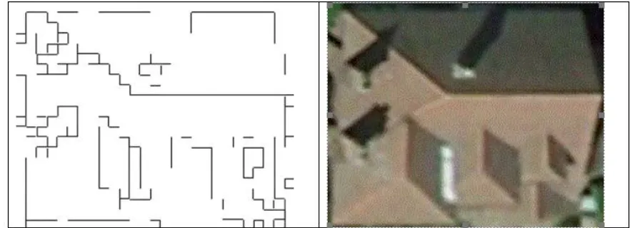
2.5 Edge Detection using Google Earth Images
213
Images captured from Google Earth were utilised because they are readily available and cover
214
all areas. Several filters available in GIMP software were investigated [36,37], including the low pass,
215
Sobel (horizontal and vertical moving windows) and Laplace (high pass). The basis of all of them is
216
gradient calculation, with edges being defined when a threshold value is exceeded, similar to the
217
Canny edge detector. The best results were achieved with the Laplace filter preceded by a 10 pixel
218
blur to prevent false edges (Figure 5).
219
220
Figure 5. Laplace (weighted high pass) filter with 10 pixel blur applied to Google Earth image of single
221
complex roof in Nottingham
222
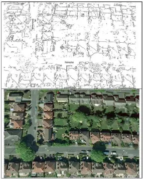
223
When a wider area was investigated (the Wollaton Park suburb surrounding the example
224
house), it became obvious that only two planes of four-plane roofs were being identified (Figure 6).
225
This image shows the south and west plane as one, and the north and east plane as one, for
226
four-plane roofs. This is possibly due to the aerial photograph being taken in the afternoon and the
227
filter merely distinguishing the sunny/less sunny sides of the roof. The next step was to investigate
228
230
Figure 6. Laplace (weighted high pass) filter with 10 pixel blur applied to Google Earth image of a
231
residential area in Nottingham
232
2.6 Image Recognition as a method of extracting roof planes
233
Initially, an unsupervised technique (i.e. image classification without the analyst’s intervention)
234
[38] was tried on the example Nottingham house. The ArcGIS software automatically groups image
235
pixels with similar values into statistically distinct classes using iterative clustering around the mean
236
(iso cluster algorithm). In this instance, the outcome was unusable. Almost every pixel in the image
237
was treated as a separate roof plane, the exception being areas of shade which were well
238
distinguished because they are much darker than the rest of the roof. Several supervised methods
239
were then tested. That is, training areas representative of separate roof planes were created by
240
manually digitising polygons. Next, these training samples were used to categorise all other pixels in
241
the image via a classification algorithm. Training examples were digitised for all directions of the
242
example Nottingham roof which may be identified manually (north, east, south and west). Areas of
243
shade on the roof and chimneys were also digitised for recognition as separate features. Two
244
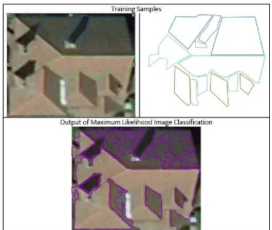
classification methods delivered reasonable results (Figure 7):
245
Class probability which employs Bayesian statistics to segment the image.
246
Maximum likelihood classification which also uses Bayes theorem but weights classes if they
247
are more likely to occur.
248
250
Figure 7. Training samples (top) and results of Maximum Likelihood Classification on Example Complex
251
Roof in Nottingham
252
253
It may be seen that again there are problems with spurious features being identified. Having
254
said that, the main difficulty is that the north plane is hard to distinguish from the east, and the
255
south plane cannot be separated from the west. This is similar to findings from edge detection of
256
Google Earth images. It appears that what is needed for accurate roof plane segmentation, is aerial
257
photographs taken at different times of the day. These images would show different roof directions
258
in slightly different colours, as the sun lights each one in sequence on its daily path. A composite
259
from several images would then deliver accurate results. However, multiple daily photographs are
260
not available from Google Earth or any other freely available image source. Therefore the decision
261
was taken to re-examine LiDAR as a data source.
262
(N.B. Google Earth’s Voyager 3D Cities layer [39] is generated from multiple sources, including
263
Sketch-up models and stereoscopic imagery. There is no 3D geometry currently accessible for
264
download, which eliminates this resource at present.)
265
2.7 Hill Shading with Ambient Occlusion applied to LiDAR as a roof segmentation method
266
The previous sections discovered a need for images captured at successive times during the
267
day. This was achieved by applying the hill shading with ambient occlusion module from SAGA
268
software [4,40–42] to 1 m LiDAR data for the residential area in Nottingham. Hill shading models
269
beam radiation from a single direction. Ambient occlusion adds the diffuse component of sunlight. It
270
samples a hemisphere around each LiDAR height point and ascertains what proportion of that
271
hemisphere is blocked by higher surrounding points. The pixel is shaded to suit. The combined
272
technique was used to generate shading patterns on roofs at different times during the day.
273
Preliminary results appear encouraging (Figure 8). North and west-facing roof planes are shaded
274
(darker) in the morning simulation (sun in southeast), north only at 2 pm, and north and east-facing
275
277
Figure 8. Hillshading with Ambient occlusion applied to a house in Nottingham at three time periods
278
279
Nonetheless, this technique has some short-comings. It does not allow for beam reflection and
280
transmission e.g. through thin cloud and therefore is not completely realistic. In addition, it is slow
281
[41].
282
2.8 Review of Progress
283
All the techniques covered so far are based on grouping the unique values allocated to each
284
LiDAR grid height point or Google Earth image pixel colouration to produce realistic roof planes.
285
That is, roof segmentation traditionally precedes estimation of solar potential on building roofs. This
286
may be the standard approach but, as illustrated above, there are many difficulties, summarised in
287
Table 1. None of the above methods works well with the data resolution available in the UK (1 m for
288
the most part). The following sections present an alternative methodology to conventional rooftop
289
PV models.
290
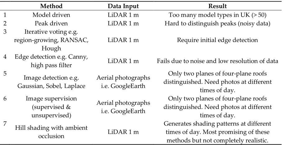
Table 1. Results of test of existing methods of rooftop PV estimation.
291
Method Data Input Result
1 Model driven LiDAR 1 m Too many model types in UK (> 50) 2 Peak driven LiDAR 1 m Hard to distinguish peaks (noisy data) 3 Iterative voting e.g.
region-growing, RANSAC, Hough
LiDAR 1 m Require initial edge detection
4 Edge detection e.g. Canny,
high pass filter LiDAR 1 m Fails due to noise and low resolution of data 5
Image detection e.g. Gaussian, Sobel, Laplace
Aerial photographs i.e. GoogleEarth
Only two planes of four-plane roofs distinguished. Need photos at different
times of day. 6 Image supervision
(supervised & unsupervised)
Aerial photographs i.e. GoogleEarth
Only two planes of four-plane roofs distinguished. Need photos at different
times of day. 7
Hill shading with ambient
occlusion LiDAR 1 m
Generates shading patterns at different times of day. Most promising of these
methods but not completely realistic.
292
3. Method to discover whether roofs are suitable for minimum size PV installation
293
Instead of beginning by segmenting roofs into planes, this method takes the following question
294
as its premise: “Is this roof suitable for PV?”. The suitability checklist has three elements: (1) azimuth
295
East through South to West; (2) space for at least a minimum size photovoltaic system (8 m2 of roof
296
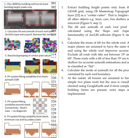
This new approach comprises the subsequent steps which are displayed graphically in Figure 9.
298
ArcGIS commands to complete the steps are listed in the Appendix.
299
300
301
1. Extract building height points only from the
302
LiDAR grid, using OS Mastermap Topography
303
layer [22] as a “cookie cutter”. That is, heights of
304
all other objects e.g. trees, cars, bus shelters are
305
removed (Figure 9, step 1).
306
2. The tilt and azimuth of each roof pixel is
307
calculated using the Slope and Aspect
308
functionality of ArcGIS software (Figure 9, step
309
2).
310
3. Calculate the mean of tilt for the whole roof. All
311
major planes are assumed to have the same tilt
312
and using the whole roof improves accuracy.
313
Exclude all roofs with tilts not between 15⁰ and
314
60⁰. Those roofs with a tilt of less than 15⁰ are too
315
shallow for accurate azimuth estimations and are
316
re-classified as “flat”.
317
4. Calculate the mode of azimuth for all the pixels
318
contained by each roof boundary.
319
5. At the outset, all houses are assumed to have
320
simple two plane roofs but the area is visually
321
checked using GoogleEarth and if more complex
322
building forms are present, extra steps are
323
implemented:
324
325
326
327
328
329
330
331
332
333
334
335
Figure 9. Method to discover whether Roofs are suitable for minimum size PV installation
336
337
a. Two plane houses: taking due North as zero degrees, if the mode is greater
338
than 270⁰ and less than 90⁰, swap by 180⁰ to obtain the south-facing plane
339
suitable for PV. Theoretically a two-plane house should have two azimuth
340
“modes” but by chance (and inaccuracies in LiDAR) one will prevail. Every
341
non-flat building must have at least two opposite aspects. (It is only
342
necessary to find one azimuth peak, not a minimum of two as in traditional
343
peak detection.)
344
b. Four plane houses: if the mode is greater than or equal to 90⁰ and less than or
345
equal to 180⁰, then add 90⁰. If the number of west-facing pixels is greater
346
than the number of east-facing pixels, take the west-facing ones. These
347
deliver a higher solar yield and it is unlikely both roof planes will have PV
348
c. Three plane houses: as for four. However, one aspect will be missing. If no
350
actual pixel values are within 10⁰ of the swapped mode, the swap is
351
abandoned.
352
d. More than four major planes – this research does not attempt to include
353
complex roof formats because these are considered unsuitable for PV.
354
6. Pick out roofs in the southern half of the compass only: East through South to West.
355
7. Select pixels within half a standard deviation of the mode (Figure 9, (step 3).
356
8. Perform a Rook’s Case connectivity check to eliminate roof areas connected diagonally (by the
357
corners) because solar panels cannot be installed in this situation (Figure 9, step 5).
358
9. Apply a minimum 10 pixel (10 of 1 × 1 m grid squares) filter to the selected pixels to remove
359
small areas (Figure 9, step 6).
360
10. Carry out a boundary clean to remove dangling pixels etc.
361
11. Size of the roof patches may be computed (see Appendix). However, all patches selected now
362
meet the minimum requirements for PV, which is the aim of this approach.
363
364
Note: for speed or in very large areas, the default of two plane roofs may be accepted. This is the
365
most common roof type for houses of all ages (see photographs by [43]). Gabled (two plane) roofs
366
are also found on terraced houses which comprise large areas of industrial cities.
367
The decision was taken to use the azimuth rather than the tilt to check for minimum PV system
368
size. Experience proved the azimuth to be subject to less minor variations than the tilt, hence it was
369
easier to aggregate pixels around a statistical value. An experiment on ten houses where the azimuth
370
could be measured revealed the mode to be the most successful statistic for aggregation. (As
371
opposed to mean, maximum etc). There is less skewing effect from errors.
372
In order to group roof pixels into areas which may be checked for minimum PV size
373
requirements, the following statistical methods were tested. These all select azimuth pixels around
374
the mode:
375
Equal interval +/- 45 degrees.
376
Jenks Natural Breaks [44]
377
Half standard deviation of mode. This collects one third of roof data (68% std/2).
378
One third standard deviation of mode. This collects about a quarter of roof data (68% std/3 =
379
23%.
380
One quarter standard deviation of mode. This collects about one sixth of roof data (68% std/4 =
381
17%).
382
These five techniques were tried on a database of housing association homes with PV installed
383
(see Section 4). 886 of the homes are covered by LiDAR flights, making them usable as test cases.
384
System size of each installation is known, so solar panel area may be calculated (1 kW = 8 m2). The
385
horizontal roof patch area selected as suitable for PV in each case was corrected to tilt area with the
386
cosine rule (see Appendix). It was found that the half standard deviation method delivered the most
387
accurate results. It failed to identify roofs as suitable for PV installation for only 2.5% of the housing
388
association homes which are already fitted with systems. The other four techniques failed about
389
twice as frequently. Manual comparison of the more complex houses in the Wollaton Park case
390
study with aerial photography also found the half standard deviation method to be preferable.
391
This method is compatible with the available LiDAR resolution and is achievable using a
392
standard desktop PC. No specialist software is required, other than GIS. The process relies on data
393
processing. Automation is possible, but not essential. Sample results for the Wollaton Park area of
394
Nottingham are illustrated in Figure 10. 40 roofs are identified as suitable for PV. Some complex
395
roofs are wrongly identified in the top right of the image. These are inappropriate for solar panels
396
because of dormers and cross gables. However, compared to the methods detailed in Section 2, this
397
399
Figure 10. Results of half standard deviation of mode method for 200 m by 200 m section of Wollaton Park
400
area of Nottingham.
401
4. Results and Validation of half standard deviation of mode method
402
The new method is validated against data from a selection of approximately 2000 domestic
403
citywide PV systems currently installed in Nottingham, UK. These are part of database of housing
404
association homes with PV installed. It was possible to obtain address (and therefore
405
latitude/longitude), system size and installers’ values of tilts and azimuths for these systems. 886 of
406
the homes are covered by LiDAR, so it is possible to compare modelled results to actual
407
on-the-ground measurements. The results are summarised in Table 2 and illustrated in Figures 11
408
and 12. Figure 11 graphs the percentage of actual systems within 5 degree bins of the modelled value
409
of tilt/azimuth. Figure 12 charts the under/over-estimation of roof plane size.
410
4.1 Tilt
411
61% of the LiDAR estimated tilts were found to be within 5⁰ of the installer’s values (Table 2).
412
87% of the LiDAR estimated tilts were within 10⁰ of the installer’s values (Figure 11). The Mean Bias
413
Error (MBE) is 4o and the Root Mean Square Error (RMSE) is 7⁰, most frequently occurring error 4⁰.
414
Given that homogeneous houses vary by 3⁰ [1], these are acceptable results. In addition, the
415
installers’ figures are thought to be “rule of thumb” and not measured e.g. by inclinometer. 10⁰ tilt
416
variation between the traditional UK roof pitches of 40-50⁰ will only make a 1% difference to average
417
annual plane-of-array irradiation received [3].
418
4.2 Azimuth
419
33% of the LiDAR estimated tilts were found to be within 5⁰ of the installer’s values (Table 2).
420
66% of the LiDAR estimated tilts were within 15⁰ of the installer’s values. 100% of the LiDAR
421
estimated tilts were within 45⁰ of the installer’s values (Figure 11). 45⁰ azimuth variance impacts
422
plane-of-array irradiation by 15%. The MBE is 14% and RMSE 18%, most frequently occurring error
423
5⁰. Again, these figures are considered to be satisfactory.
424
Tolerable results have been achieved despite the fact that difficulties were noted with the
425
housing association dataset. Visual checks using GoogleEarth discovered cases where the LiDAR
426
derived figure is correct and the installers’ value is not. Tilts and azimuths appear to have been
427
transposed in the database in some instances. Additionally, the installers appear to have estimated
428
azimuth by the position of the sun without allowing for its annual path.
429
431
4.3 Roof Patch Area
432
97.5% of established systems used in the validation process were correctly identified as being
433
suitable for at least a minimum potential 1 kW system (Figure 12). 80% had an area at least the size of
434
the actual installed system. Comparing LiDAR derived values and values calculated from the
435
system sizes, the MBE is 6% and RMSE 9%.
436
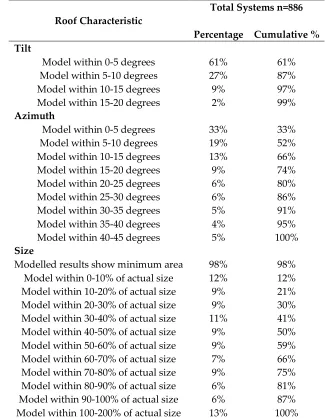
Table 2. Results of validation of half standard deviation of mode method.
437
Roof Characteristic
Total Systems n=886
Percentage Cumulative % Tilt
Model within 0-5 degrees 61% 61%
Model within 5-10 degrees 27% 87%
Model within 10-15 degrees 9% 97%
Model within 15-20 degrees 2% 99%
Azimuth
Model within 0-5 degrees 33% 33%
Model within 5-10 degrees 19% 52% Model within 10-15 degrees 13% 66%
Model within 15-20 degrees 9% 74%
Model within 20-25 degrees 6% 80%
Model within 25-30 degrees 6% 86%
Model within 30-35 degrees 5% 91%
Model within 35-40 degrees 4% 95%
Model within 40-45 degrees 5% 100%
Size
Modelled results show minimum area 98% 98% Model within 0-10% of actual size 12% 12% Model within 10-20% of actual size 9% 21% Model within 20-30% of actual size 9% 30% Model within 30-40% of actual size 11% 41% Model within 40-50% of actual size 9% 50% Model within 50-60% of actual size 9% 59% Model within 60-70% of actual size 7% 66% Model within 70-80% of actual size 9% 75% Model within 80-90% of actual size 6% 81% Model within 90-100% of actual size 6% 87% Model within 100-200% of actual size 13% 100%
438
440
441
Figure 11. Distribution of difference in tilt and azimuth.
442
443
444
445
Figure 12. Distribution of difference in size.
446
4.4 Review of Validation
447
Table 2 and Figures 11 and 12 show that the majority of the modelled tilt and azimuth values
448
fall within 15-20 degrees (6%) of the installers’ values. However, the spread of size value differences
449
is much wider. Only 12% of results are within 10% of the ground-measured value. Therefore this
450
research concentrates on identifying suitability for a minimum size PV system only, with 98%
451
accuracy.
452
4.5 Context of half standard deviation of mode method.
453
Comparable techniques have been developed by [16] and NREL [14,45,46]. This section
454
[16] bin individual pixel values from LiDAR into seven slope (tilt) and five aspect (azimuth)
456
classes. The results are smoothed by replacing pixel values based on the majority of a 3 × 3
457
neighbourhood to the present pixel (Majority Filter). Prior classification means that the fine detail of
458
the original input LiDAR is lost during the roof segmentation. This work is validated visually by
459
matching 150 rooftops in Philadelphia to aerial imagery.
460
Similar to [16], NREL categorize each 1 × 1 m roof square into nine azimuth classes. For each
461
distinct roof plane creating by azimuth classification, the mean tilt was determined (Zonal Mean). A
462
PV installer’s data set containing the location, tilt and azimuth of 205 assembled PV arrays was used
463
to validate the results of this analysis.
464
[16] report that their method gives the most precise results when applied to simple roof
465
structures. NREL’s technique has virtually the same accuracy as the half standard deviation of mode
466
method. 89% of NREL modelled results were within 10⁰ of the actual slope compared to 87%
467
obtained by the current authors. 96% of NREL’s modelled results have the same azimuth as the
468
actual azimuth set against the 100% accuracy obtained by the current authors (allowing for
469
categorization into compass bands to be compatible with NREL).
470
The techniques of [16] (prior classification with Majority Filter) and NREL (single tilt value for
471
each unique roof plane obtained from the azimuth) were tested with UK data. It was found that the
472
Majority Filter did not add any accuracy. Straightforward categorization into compass band as
473
previously carried out by the current authors [3] gives greater accuracy in the UK. This is due to the
474
low number of LiDAR pixels which fall inside the boundary of a typical UK home. Likewise,
475
calculating the tilt value for every roof plane generated flawed results because segmenting small
476
buildings gives inaccurate results due to lack of data points.
477
The methods of [16] and NREL are reported as working well for the larger homes of the US. The
478
method presented here (entire building average for tilt and half standard deviation of mode for
479
azimuth planes) is suitable for the smaller houses of the UK and other European and Asian
480
countries. It is validated against more actual buildings’ data than any previous method.
481
5. Research Summary and Discussion
482
The tool developed here can be a powerful resource for investigating the deployment of rooftop
483
PV. It can assist network operators in understanding how much energy the UK’s potential minimum
484
number of solar panels can produce and improve the efficiency of the electricity network.
485
It does not focus on obtaining accurate values of tilt, azimuth and roof area but simply asks, “is
486
this roof suitable for PV installation?”. Thus, the minimum PV capacity for any city region may be
487
estimated and hence minimum solar yield. The maximum sized systems may not be installed on
488
houses in any event, due to cost, aesthetics or fairness between rented properties.
489
The new method works on the basis of selecting pixels within half a standard deviation of the
490
azimuth mode. The mode is the value at which the peak of the distribution curve occurs. It is a
491
flexible approach to handling non-ideal data, where standard peak finding algorithms cannot cope
492
with the noise. The end result is a map of roofs suitable for PV system installation; size at least 1 kW,
493
known tilt and azimuth. These results can be aggregated by region to calculate minimum potential
494
yield per area.
495
This technique has been comprehensively validated using two techniques. Firstly, by a check
496
for wrongfully selecting inappropriate roofs as suitable for PV. This was carried out by manually
497
matching 50 rooftops in Wollaton Park to GoogleEarth imagery (Figure 10). Two roofs were
498
incorrectly selected as opposed to 50 correctly categorized. Secondly, by a check for missing suitable
499
roofs by comparison against the biggest installation database used by any analogous research to
500
date.
501
5. Conclusions
502
This method is useful, effective and functions correctly with the data publicly available in the UK
503
this respect, it provides a valuable contribution to the scientific field because the methods tested and
505
reviewed in Section 2 require higher resolution input data than can be provided to produce usable
506
results.
507
The unique attribute of the method presented here is that it is twice validated, by extensive
508
ground-truthing against a database of 886 installations, and against aerial photography. This makes
509
it the most thoroughly validated method to date.
510
The aim of any PV roof-area estimation method is to provide data for further analysis. This method
511
is flexible. It allows individual houses as well as large numbers of properties to be examined,
512
depending upon later requirements. Unlike some methods, it makes no assumptions when larger
513
numbers are involved and does not rely on compass band classification. An example of use of the
514
data generated would be a study of the relationship between azimuth and self-consumption. A
515
range of PV-related research is enabled.
516
Author Contributions: Conceptualization, Diane Palmer, Ian Cole and Ralph Gottschalg; Data curation, Diane
517
Palmer and Elena Koubli; Formal analysis, Diane Palmer; Funding acquisition, Ralph Gottschalg; Investigation,
518
Diane Palmer; Methodology, Diane Palmer; Project administration, Diane Palmer; Resources, Diane Palmer;
519
Software, Diane Palmer; Supervision, Ralph Gottschalg and Thomas Betts; Validation, Diane Palmer;
520
Visualization, Diane Palmer; Writing – original draft, Diane Palmer; Writing – review & editing, Thomas Betts.
521
Funding: This work has been conducted as part of the research projects ‘PV2025 - Potential Costs and Benefits
522
of Photovoltaic for UK Infrastructure and Society’ and ‘Joint UK-India Clean Energy Centre (JUICE)’ which are
523
funded by the RCUK's Energy Programme (contract no: EP/K02227X/1 and contract no: EP/P003605/1). The
524
projects funders were not directly involved in the writing of this article.
525
Conflicts of Interest: The authors declare no conflict of interest.
526
Appendix A
527
ArcGIS Commands for method to discover whether roofs are suitable for minimum size PV
528
installation:
529
1. Preparation: Subtract Environment Agency digital terrain (DTM) LiDAR from the
530
digital surface model (DSM) to obtain building height above ground level. Delete pixels
531
with a lower height than 2 m. This removes rogue values whilst allowing for low eaves.
532
2. Cut out buildings only. Prepared LiDAR DSM-DTM grid and buildings from OS
533
Mastermap Topography layer as inputs: ArcToolbox > Spatial Analyst > Extraction >
534
Extract by Mask
535
3. Spatial Analyst > Surface > Slope / Aspect. Create integer rasters to enable mode to be
536
computed in the next step.
537
4. Spatial Analyst Tools > Zonal > Zonal Statistics > Mean
538
5. Spatial Analyst Tools > Zonal > Zonal Statistics > Mode
539
6. Mode may be in the north, so carry out some swaps:
540
a. Swap mode raster values by 180:
541
Raster calculator:
542
i. Values between 90 and 270 are alright:
543
Con(("aspectmode" <= 270) & ("aspectmode" >= 90), "aspectmode", 0)
544
ii. Values between 0 and 90:
545
Con(("aspectmode" <= 90) & ("aspectmode" >= -1), ("aspectmode" +180), 0)
546
iii. Values between 270 and 360:
547
Con(("aspectmode" <= 360) & ("aspectmode" >= 270), ("aspectmode" -180), 0)
548
iv. "PVMode" = "Con1" + "Con2" + "Con3"
549
b. Optionally, switch by 90 east to west for 4-plane houses:
550
Con(("Con4" >= 90) & ("Con4" <= 160), ("Con4" +90), "Con4")
551
c. If the west mode generates a bigger polygon than the east, take that.
552
Con(("intaspect" >= "PVMode" - "StdAspect" / 2) & ("intaspect" <= "PVMode" +
554
"StdAspect" / 2),1,0)
555
This makes a 1,0 raster of cells half std around the mode.
556
8. Connectivity: ArcToolbox > Spatial Analyst Tools > Generalisation > Region Group
557
Four neighbours (for edges only, Rooks Case), Cross – exclude zero (“0”).
558
9. Select Large Enough Areas
559
From Count because 1 × 1 m pixels. Reclassify as in Table A1 below and discard highest
560
number which is areas not suitable for PV.
561
Table A1. Reclassification of pixel values to enable selection of roof area of at least 8m2.
562
Old Values New Values
1-9 NoData
9-19 2
19-30 3
30-44 4
44-63 5
63-96 6
96-175 7
175-302 8
> 302 NoData
NoData NoData
563
10. Clean: Spatial Analyst Tools > Generalisation > Boundary Clean
564
No sort, run twice.
565
11. Measure Roof Patch with homogeneous aspect (azimuth):
566
Zonal statistics sum points in raster.
567
(Add all the “1”s, not zeroes because “1”s are 1 m squares).
568
12. To calculate a more accurate area allowing for the roof tilt:
569
Slope distance = horizontal distance/cosine(Tilt in degrees)
570
E.g. Slope distance = 21.2 m / cos [32⁰]
571
References
572
1. European Commission. EU Buildings Database. Policies, Inf Serv 2015:1–29.
573
https://ec.europa.eu/energy/en/eu-buildings-database (accessed September 4, 2018).
574
2. Gagnon P., Margolis R., Melius J., Phillips C., Elmore R. Rooftop Solar Photovoltaic Technical Potential in
575
the United States: A Detailed Assessment. Golden, Colorado: 2016.
576
https://www.nrel.gov/docs/fy16osti/65298.pdf
577
3. Palmer D., Cole I., Betts T., Gottschalg R. Assessment of potential for photovoltaic roof installations by
578
extraction of roof tilt from light detection and ranging data and aggregation to census geography. IET
579
Renew Power Gener 2016; 10:467–73. doi:10.1049/iet-rpg.2015.0388.
580
4. Palmer D., Cole I., Goss B., Betts T., Gottschalg R. Detection of roof shading for PV based on LiDAR data
581
using a multi-modal approach. In: Wendlandt S, Berthold R, Stegemann B, Suchaneck O, Hanusch M,
582
Drobisch A, et al., editors. 31st Eur. Photovolt. Sol. Energy Conf. Exhib., Hamburg: 2015, p. 2477–81.
583
5. Goss B., Cole I.R., Koubli E., Palmer D., Betts T.R., Gottschalg R. 4 - Modelling and prediction of PV
584
module energy yield. In: Nicola Pearsall (Northumbria University), editor. Perform. Photovolt. Syst.
585
Model. Meas. Assess. First, Elsevier Ltd.; 2016, p. 103–34. doi:10.1016/B978-1-78242-336-2.00004-5.
586
6. DBEIS. Solar photovoltaics deployment. Natl Stat 2018:1–7.
587
https://www.gov.uk/government/statistics/solar-photovoltaics-deployment (accessed September 4, 2018).
588
7. Masson G., Kaizuka I. Trends 2017 in Photovoltaic Applications. Report IEA PVPS T1-32:2017. Survey
589
Report of Selected IEA Countries between 1992 and 2016, edition 22.
590
https://www.researchgate.net/publication/324728347_TRENDS_2017_IN_PHOTOVOLTAIC_APPLICATI
591
8. Riksdienst voor Ondernemend Nederland. International Positioning of the Dutch PV Sector. Final Report
593
for Publication. 2014.
594
https://www.rvo.nl/sites/default/files/2014/08/International%20positioning%20of%20the%20Dutch%20PV
595
%20sector%20final.pdf
596
9. Liu Y. Solar PV in China Looks Promising for 2018. Renew Energy World 2018:1.
597
https://www.renewableenergyworld.com/articles/2018/03/solar-pv-in-china-looks-promising-for-2018.ht
598
ml (accessed November 19, 2018)
599
10. Hafez A.Z., Soliman A., El-Metwally K.A., Ismail I.M. Tilt and azimuth angles in solar energy applications
600
– A review. Renew Sustain Energy Rev 2017;77:147–68.
601
https://www.researchgate.net/...angle...tilted.../10.1016%40j.rser.2017.03.131.pdf
602
11. Hartner M., Ortner A., Heisl A., Haas R. East to west – The optimal tilt angle and orientation of
603
photovoltaic panels from an electricity system perspective. Appl Energy 2015;160:94–107. Doi:
604
https://doi.org/10.1016/j.apenergy.2015.08.097.
605
12. Davies J. A Guide To Roof Construction – Part 1. Gt Home 2013:1.
606
great-home.co.uk/a-guide-to-roof-construction/ (accessed November 19, 2018
607
13. Vaughn T.G.I. What is the typical roof pitch on a mediterranean style home? Houzz 2017:1.
608
https://www.houzz.com/discussions/4046877/what-is-the-typical-roof-pitch-on-a-mediterranean-style-ho
609
me (accessed September 6, 2018).
610
14. Melius J., Margolis R., Ong S. Estimating Rooftop Suitability for PV : A Review of Methods, Patents , and
611
Validation Techniques 2013:35.
612
https://digital.library.unt.edu/ark:/67531/metadc866924/m2/1/high_res_d/1117057.pdf
613
15. Hong T., Lee M., Koo C., Jeong K., Kim J. Development of a method for estimating the rooftop solar
614
photovoltaic (PV) potential by analyzing the available rooftop area using Hillshade analysis. Appl Energy
615
2017;194:320–32. https://www.sciencedirect.com/science/article/pii/S0306261916309424
616
16. Boz B.M., Calvert K., Brownson J.R.S. An automated model for rooftop PV systems assessment in ArcGIS
617
using LIDAR. AIMS Energy 2015;3:401–20.
618
www.aimspress.com/article/10.3934/energy.2015.3.401/fulltext.html
619
17. Campana P.E., Quan S.J., Robbio F.I., Lundblad A., Zhang .Y, Ma T., et al. Optimization of a residential
620
district with special consideration on energy and water reliability. Appl Energy 2017;194:751–64.
621
https://www.researchgate.net/publication/309333789_Optimization_of_a_residential_district_with_special
622
_consideration_on_energy_and_water_reliability
623
18. Ordonez J., Jadraque E., Alegre J., Martinez G. Analysis of the Photovoltaic Solar Energy Capacity of
624
Residential Rooftops in Andalusia (Spain). Renew Sustain Energy Rev 2010;14:2122–30.
625
https://www.sciencedirect.com/science/article/pii/S136403211000002X
626
19. Environment Agency. Survey Open Data n.d. http://environment.data.gov.uk/ds/survey/#/survey
627
(accessed January 11, 2018).
628
20. Google Earth Pr9 V7.3.2.5491. (2018). Nottingham, U.K. DigitalGlobe 2012.
629
http://www.google.com/earth/download/ge/
630
21. Laporte J. What Size Solar Panel Do I Need For My Home? - The Eco Experts n.d.
631
https://www.theecoexperts.co.uk/solar-panels/what-size-do-i-need (accessed November 13, 2018).
632
22. Ordnance Survey. OS MasterMap Topography Layer 2014.
633
https://www.ordnancesurvey.co.uk/business-and-government/products/topography-layer.html (accessed
634
June 10, 2017).
635
23. Burrough P.A., McDonell R.A. Principles of Geographical Information Systems. New York: Oxford
636
University Press; 1998.
637
24. Jacques D.A., Gooding J., Giesekam J.J., Tomlin A.S., Crook R. Methodology for the assessment of PV
638
capacity over a city region using low-resolution LiDAR data and application to the City of Leeds (UK).
639
Appl Energy 2014;124:28–34. doi:10.1016/j.apenergy.2014.02.076.
640
25. Wikipedia. List of roof shapes. Wikipedia 2018:1. https://en.wikipedia.org/wiki/List_of_roof_shapes.
641
26. Ballard S., Dibb M., Facey P., Hunter B., Johnstone C., Stott R. Geograph Britain And Ireland 2005.
642
http://www.geograph.org.uk (accessed January 11, 2018).
643
27. Stilla U., Jurkiewicz K. Automatic reconstruction of roofs from maps and elevation data. Int Arch
644
Photogramm Remote Sens 1999;32:4–3.
645
28. Lukač N., Žlaus D., Seme S., Žalik B., Štumberger G. Rating of roofs’ surfaces regarding their solar potential
647
29. Demir N., Baltsavias E. Automated Modeling of 3D Building Roofs Using Image and Lidar Data. ISPRS
648
Ann Photogramm Remote Sens Spat Inf Sci 2012;I-4:35–40. doi:10.5194/isprsannals-I-4-35-2012.
649
30. Tarsha-Kurdi F., Landes T., Grussenmeyer P., Koehl M. Model-Driven and Data-Driven Approaches Using
650
Lidar Data : Analysis and Comparison. PIA07 - Photogramm Image Anal 2007;36:87–92.
651
https://halshs.archives-ouvertes.fr/file/index/docid/264846/filename/Tarsha_TL_PG_MK_PIA_07.pdf
652
31. Canny J. A computational approach to edge detection. IEEE Trans Pattern Anal Mach Intell 1986;8:679–98.
653
http://citeseerx.ist.psu.edu/viewdoc/download?doi=10.1.1.420.3300&rep=rep1&type=pdf
654
32. GRASS Development Team. Geographic Resources Analysis Support System (GRASS) Software 2015.
655
https://grass.osgeo.org/
656
33. Conrad O., Bechtel B., Bock M., Dietrich H., Fischer E., Gerlitz L., et al. System for Automated Geoscientific
657
Analyses (SAGA) v. 2.1.4. Geosci Model Dev 2015;8. doi:10.5194/gmd-8-1991-2015.
658
34. ESRI. ArcGIS Desktop: Release 10.3 2014.
659
https://support.esri.com/en/products/desktop/arcgis-desktop/arcmap/10-3
660
35. ESRI. How Filter works—Help | ArcGIS for Desktop n.d.
661
http://desktop.arcgis.com/en/arcmap/10.3/tools/spatial-analyst-toolbox/how-filter-works.htm (accessed
662
January 11, 2018).
663
36. The GIMP team, GIMP 2.8.10, www.gimp.org, 1997-2014, retrieved on 31.07.2014
664
37. The GIMP Team. Chapter 17. Filters n.d. https://docs.gimp.org/en/filters.html (accessed January 11, 2018).
665
38. ESRI. What is image classification?—ArcGIS Help | ArcGIS Desktop n.d.
666
http://desktop.arcgis.com/en/arcmap/latest/extensions/spatial-analyst/image-classification/what-is-image-667
classification-.htm (accessed January 11, 2018)
668
39. Romaszewicz, M. How are the 3D models of buildings generated on Google Earth? Where did they get all
669
this data, and how was it compiled? n.d.
670
https://www.quora.com/How-are-the-3D-models-of-buildings-generated-on-Google-Earth-Where-did-the
671
y-get-all-this-data-and-how-was-it-compiled (accessed January 11, 2018).
672
40. Tarini M., Cignoni P., Montani C. Ambient Occlusion and Edge Cueing for Enhancing Real Time Molecular
673
Visualization. IEEE Trans Vis Comput Graph 2006;12:1237–44. doi:10.1109/TVCG.2006.11
674
41. Kay S. A recipe for hillshading with QGIS and SAGA. Stevefaeembra Blog 2015:1.
675
http://www.stevefaeembra.com/blog/2015/8/1/a-recipe-for-hillshading-with-qgis-and-saga (accessed
676
September 7, 2018).
677
42. Conrad O., Wichmann V. SAGA-GIS Module Library Documentation (v2.2.1) 2013:1.
678
http://www.saga-gis.org/saga_tool_doc/2.2.1/ta_lighting_0.html
679
43. Barrow M. Project Britain Houses. Proj Britain 2013:1. http://projectbritain.com/. (accessed September 4,
680
2018)
681
44. Jenks G.F., Caspall F.C.. Error on choroplethic maps: Definition, measurement, reduction. Ann Am Geogr
682
1971;61:217–44. https://www.tandfonline.com/doi/abs/10.1111/j.1467-8306.1971.tb00779.x
683
45. R.G., Margolis .P, Melius R., Phillips J., Elmore C. Rooftop Solar Photovoltaic Technical Potential in the
684
United States: A Detailed Assessment. 2016. https://www.osti.gov/biblio/1236153
685
46. Margolis R., Gagnon P., Melius J., Phillips C., Elmore R. Using GIS-based methods and lidar data to
686
estimate rooftop solar technical potential in US cities. Environ Res Lett 2017;12:1–7.
687
http://iopscience.iop.org/article/10.1088/1748-9326/aa7225/meta
688