http://www.sciencepublishinggroup.com/j/se doi: 10.11648/j.se.20190704.11
ISSN: 2376-8029 (Print); ISSN: 2376-8037 (Online)
Review Article
A Review on Surrogate-Based Global Optimization Methods
for Computationally Expensive Functions
Pengcheng Ye
1, 21
School of Marine Science and Technology, Northwestern Polytechnical University, Xi'an, China 2
Key Laboratory for Unmanned Underwater Vehicle, Northwestern Polytechnical University, Xi’an, China
Email address:
To cite this article:
Pengcheng Ye. A Review on Surrogate-Based Global Optimization Methods for Computationally Expensive Functions. Software Engineering. Vol. 7, No. 4, 2019, pp. 68-84. doi: 10.11648/j.se.20190704.11
Received: October 2, 2019; Accepted: October 21, 2019; Published: November 19, 2019
Abstract:
The great computational burden caused by complicated and unknown analysis restricts the use of simulation-based optimization. In order to mitigate this challenge, surrogate-based global optimization methods have gained popularity for their capability in handling computationally expensive functions. This paper surveys the fundamental issues that arise in Surrogate-based Global Optimization (SBGO) from a practitioner’s perspective, including highlighting concepts, methods, techniques as well as engineering applications. To provide a comprehensive discussion on the issues involved, recent advances in design of experiments, surrogate modeling techniques, infill criteria and design space reduction are investigated. This review screens out nearly 130 references containing a lot of historical reviews on related research fields from about 500 publications in various subjects. Future challenges and research is also analyzed and discussed.Keywords:
Global Optimization, Surrogate Models, Review, Computationally Expensive Functions, Future Challenges1. Introduction
With the globalization of trade, all industrial companies are faced with the worldwide competition and strive to produce cheaper and better products faster. These processes and products can be optimized with various objectives like quality, cost and time, etc. In many fields such as aircraft design, the complex systems encompass the extensive activities whose goal is to determine the optimum characteristics of a product before it is manufactured. Thus, it accelerates the advancement of global optimization approaches. Generally, global optimization methods can be classified into two main categories: deterministic and stochastic [1]. Deterministic global optimization methods will gradually converge to the global optimum through generating a deterministic sequence of points. It can only solve the optimization problems which have certain mathematical characteristics like gradient information though the global optima may be found rapidly. In practice, the special mathematical characteristics perhaps not exist in most simulation assisted global optimization problems. Moreover, the stochastic or called derivative-free global
optimization methods solve the aforementioned computation-intensive optimization problems through the random generation of feasible points. Rios and Sahinidis[2] present a review of many widely used derivative-free global optimization methods. Thereinto, the popularity of traditional derivative-free global optimization methods including Genetic Algorithm (GA), Simulated Annealing (SA) and Particle Swarm Optimization (PSO) lies in the ease of implementation and flexible way [3, 4].
optimization is in direct proportion to the number of function evaluations. An intuitive way to relieve this difficulty within limited computational budgets is to use surrogate models to replace the expensive black-box analysis, termed as surrogate-based global optimization. SBGO methods have been extensively employed for handling the computationally expensive unknown problems such as aerospace, vehicle, and power system designs. Younis et al. [6] use a novel space exploration and unimodal region elimination global optimization algorithm to solve a highly nonlinear and complex real-life engineering design optimization problem-the optimal design of automotive magnetorheological brake. Sun et al. [7] adopt Kriging (KRG) model to replace expensive CFD code for calculating the hydrodynamic performance of the underwater glider. Lee et al. [8] develop a surrogate-based design optimiztion framework to maximize the thrust coefficient of multiple wing sails. Mainini and Willcox [9] propose an offline/online strategy for the data-to-decision problem of onboard structural assessment. Peherstorfer et al. [10] present a multi-fidelity method to importance sampling that leverages multiple surrogate models for speeding up the construction of a biasing distribution and that uses the high-fidelity model to derive an unbiased estimate of the failure probability.
SBGO is an excellent technique and possesses several advantages compared to the traditional optimization method [11, 12]. The distinct advantages of SBGO are given as follows:
It requires fewer resource and time due to the approximation process;
It can better utilize the information collected from the available samples;
It contributes to provide insights into the expensive black-box problems by studying the sensitivity of design variables;
It is easier to filter the noise intrinsic to numerical and experimental data;
It supports parallel computation.
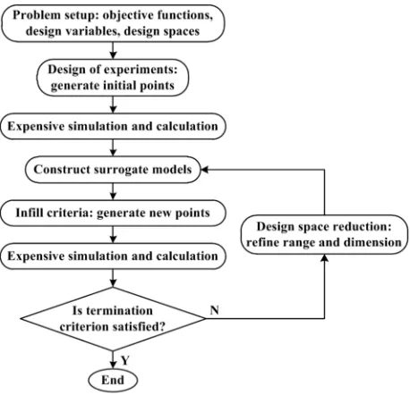
Figure 1. General framework of SBGO.
The basic framework for most SBGO is illustrated in Figure 1. It can be found that four key components including Design of Experiments (DOE), surrogate modeling techniques, infill criteria and design space reduction are the key issues which arise in surrogate-based global optimization. This optimization process starts with generating an initial sample set through using a certain design of experiments method. The obtained sample data are employed to construct the first surrogate model. It’s no doubt that the accuracy of surrogate models is directly affected by the performance of sample points. In recent decades, various DOE has been developed for experiments design. The classical DOE contains factorial designs, Central Composite Designs (CCD) and Orthogonal Designs (OD) [13-15]. Moreover, space-filling DOE including Uniform Designs (UD), Latin Hypercube Designs (LHD), Optimal Latin Hypercube Designs (OLHD) are widely used in surrogate-based global optimization [16-19]. Different criteria towards space-filling including Minimax and Maximin designs, Kullback-Leibler designs, Audze-Eglais designs, maximum entropy designs [20]. The optimal space-filling DOE which integrates regular DOE with above design criteria is seeking to obtain the better space-filling and projective property. Among the optimal DOE, optimal LHD is most frequently studied. Jin et al. [21] present an optimal LHD using an Enhanced Stochastic Evolutionary (ESE) algorithm. It is efficient and flexible in terms of the computation time, the number of exchanges needed for generating new designs and the various design criteria. Viana et al. [22] use the translational propagation algorithm to obtain near optimal LHD without going through the expensive optimization process, whereas the performance of the sample points is not suitable for high dimensions. The aim in this step is to generate better initial sample points to construct more accurate initial surrogate model. A review on design of experiments is presented in Section 2.
natural-laminar-flow wing in the transonic regime. Wang et al. [27] introduce a mode-pursing sampling method that can systematically generates more sample points in the neighborhood of the function mode. The sampling and detection process will iterate until the global optima are found. Holmström [28] presents a novel adaptive radial basis function method to overcome the difficulty that RBF interpolation is sensitive to the static choice of target values and initial sample points. Zhao et al. [29] propose a new method named dynamic KRG to solve the computationally intensive engineering application problems.
As is known to all, a variety of surrogate modeling techniques are developed along with the extensively employed for expensive black-box design optimization. Different surrogate models adopted have their own advantages and disadvantages which are suitable for different applications. There is no conclusion on which model is predicatively superior to the others so far. In practice, most researchers usually choose the specific surrogate models in view of the past experience from dealing with the similar real-world applications. However, it will produce the uncertainties in predictions and extra expensive computation owing to the improper choice of surrogate modeling techniques. As a weighted combination of multiple surrogate models, ensemble of surrogates is developed to relieve this conflict. This strategy is very attractive in engineering design optimization since it can gain as much information on the black-box problems as possible. It acts like an insurance policy against poorly approximate models which can eliminate the negative impact and enhance the overall prediction performance. Zerpa et al. [30] propose the use of a weighted average surrogate model for the alkali-surfactant-polymer flooding process optimization. They recommend that ensemble of surrogates performs better modeling capabilities than single surrogate models. Goel et al. [31] explore various ensemble strategies where the weights are determined using the global cross-validation error measure. Acar and Rais-Rohani [32] determine the weight factors by minimizing the Root Mean Square Error (RMSE) and Generalized Mean Square Cross-validation Error (GMSE), separately. The selection of weights is treated as an optimization problem for minimizing the specific error metric. The trouble in this step as well as the interest is the question what surrogate models should be used. An introduction on this problem is discussed in Section 3.
For improving the prediction accuracy of surrogate model, new sample points are required. The strategies for deciding the next promising samples is termed infill criteria also called adaptive sampling design method. The infill criteria can well guide the selection of new sample points depending on the information from the optimization process which will be sufficiently utilized. Infill criteria can be roughly classified as exploitation, exploration, combined exploitation and exploration. One side, the exploitation methods intuitively focus on the regions that locate in a neighborhood of the best point that has been found so far, which may not even be a stationary point of the true function. It will lead to a local
approximation and may fall into the local optimum. On the other side, the exploration methods generally explore the sparse regions or regions with high uncertainty. However, only using the exploration strategy may result in a waste of computational resource to blindly improve the global approximation accuracy. The high accuracy is mainly required in the potentially promising regions. Therefore, it’s suggested to combine exploitation and exploration to balance the competing targets between the less cost and the more accurate optimal solution [33]. Various infill criteria have been developed for choosing the new sample points in recent years. The expected improvement [34, 35] and its modified versions including weighted expected improvement [36] augmented expected improvement [37] and probability expected improvement [38] are widely used as infill criteria. This step to select further designs that offer improvement is iterative till a certain convergence criterion or termination criterion is reached. The detail of infill criteria playing an important role in SBGO is given in Section 4.
Regardless of the abovementioned optimization tools used to handle a specific problem, it’s found that the optimization efficiency and prediction accuracy are related to the scale of the design space. The difficulty that the computational demand increases exponentially while the number of design variables increases is known as the curse of dimensionality. Reducing the design space is an active and better way to overcome this difficulty. Wang and Simpson [39] use the Fuzzy C-Means (FCM) clustering approach to systematically capture the promising design space and efficiently identify the global minimum in the reduced design space. Meanwhile, FCM is also employed to determine an attractive reduced design space [40, 41]. Shyy et al. [11] discuss the fundamental issues that arise in surrogate-based modeling and dimension reduction methods for multi-scale mechanics problems. Galbally et al. [42] present an application of nonlinear model reduction to an inverse problem solution in a Bayesian inference setting. The inherent multiple-query context of the Bayesian approach makes model reduction an attractive option for large-scale problems. Shan and Wang [43] provide a review on modeling and optimization methods for solving the high-dimensional problems. A discussion on design space reduction methods in SBGO is offered in Section 5.
2. Design of Experiments
The first step for a successful application of SBGO is the planning of the initial sample points for evaluation. The information at these points is usually limited for black-box problems. Good choices of experimental designs contribute to improve the accuracy of approximate models as well as to avoid exceeding the computational budget [22, 44]. In the early days of experiment designs, DOE methods are mainly applied to physical experiments. With the advancement of the computer, many DOE approaches are developed for computer experiments. The design of physical experiments and computer experiments methods are introduced in this section. The design of physical experiments methods are firstly discussed as below.
2.1. Design of Physical Experiments
Design of physical experiments methods are focusing on the planning experiments such that the damage of the random error in physical experiments can be minimized. Popularly used physical experimental designs including factorial designs, central composite designs, orthogonal designs are described. 2.1.1. Factorial Designs
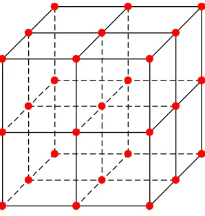
Factorial designs method classified into full factorial designs and fractional factorial designs is a simple and straightforward way to generate sample points in the uniform manner [45]. Thereinto, full factorial designs divide each dimension of the entire design space (k factors) into equal intervals (m levels) and the number of points is mk. For example, the commonly used full factorial designs are 2k or 3k with k factors at 2 and 3 levelsthat are used to evaluate main effects and interactions or quadratic effects and interactions separately [46]. Figure 2 shows a 33 full factorial design.
The size of full factorial designs increases exponentially with the number of input variables. Therefore, it’s notoriously inefficient as not a few factors are involved. This drawback prohibits the use of full factorial designs for expensive high-dimensional problems. In practice, only a fraction of points specified by full factorial designs are used that are defined as fractional factorial designs. A 33 fractional factorial design is illustrated in Figure 3. Mukerjee and Wu [47] present a detailed discussion of factorial designs.
Figure 2. 33 full factorial design.
Figure 3. 33 fractional factorial design.
2.1.2. Central Composite Designs
CCD is firstly developed by Box and Wilson [48], which is the most popular family of second-order response surface designs. CCD is a two level factorial design (2k) that is augmented by c0 center points and 2k axial points positioned at
a distance of α from the center. For a three factors design, the total amount of points is 14+ c0 which c0 is a replication
number of center points. It’s noticeable that the parameters c0
and α need to be predefined for CCD. A CCD for three variables is shown in Figure 4.
Figure 4. Central composite design.
The central composite designs can extract almost as much information as a multilevel full factorial designs which require fewer experiments and also have been certified to be sufficient to describe the majority of steady-state process responses [49]. This method allows researchers to visualize the interaction among independent factors under different experimental conditions. The central composite designs have been partly used despite the fact that the amount of points still increases exponentially with the number of design variables as well as the factorial designs [50, 51].
2.1.3. Orthogonal Designs
Orthogonal designs contain a number of orthogonal runs which can be generated by orthogonal array. Promotion of the application of orthogonal designs is greatly owing to the work of Taguchi [52, 53] in quality engineering. The general form of orthogonal designs is u
( )
b a
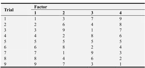
indicates the integer series, au represents the total amount of experiment runs. The relation between these parameters can be formulated as b=(au–1)/(a–1). For instance, an orthogonal design with 9 trails, 3 levels and 4 factors expressed as L9 (34)
is exhibited in Table 1. Orthogonal designs treat all regions equally and can reduce the number of design points. Moreover, it may limit factors moving to narrower ranges. However, it is unable to know a priori which factors are crucial. Orthogonal designs also may result in replication of points and lack of flexibility. Detail introduction on orthogonal designs can refer to these publications [54-56].Hou et al. [57] employ factorial designs to screen active parameters for optimizing a new thin-walled cellular configuration. Wang et al. [58] propose an adaptive response surface method that creates a quadratic polynomial approximation model to deal with the expensive back-box problems in a reduced space obtained by using central composite designs. Gong et al. [59] incorporate the orthogonal designs into differential evolution for accelerating its convergence rate. Recent studies on the design of physical experiments are developed [60-62].
Table 1. Orthogonal design of L9 (34).
Trial Factor
1 2 3 4
1 1 1 1 1
2 1 2 2 2
3 1 3 3 3
4 2 1 2 3
5 2 2 3 1
6 2 3 1 2
7 3 1 3 2
8 3 2 1 3
9 3 3 2 1
2.2. Design of Computer Experiments
The random error will occur during physical experiments. As a result, the designs of physical experiments prefer to distribute the points around the boundaries of design space for reducing the random error through reduplicative tests at the same settings. However, the computer experiments mainly involve systematic error rather than the random error and mostly spread the points to fill the whole space which are also called space-filling designs. It’s different from the physical experiments. Simpson et al. [63] confirm that the conventional physical experimental designs are inefficient or even improper for computer experiments. In order to extract more information of the expensive black-box functions with least number of samples, a large amount of computer experimental designs are developed to meet the space-filling property. Several designs of computer experiments strategies including uniform designs, Latin hypercube designs and optimal Latin hypercube designs are introduced as below.
2.2.1. Uniform Designs
Uniform designs have been widely used since Fang [64] introduced them to experimental design terminology. It treats all regions equally and offer uniformly scatter points in the design space. UD is a type of optimal design incorporated with
a supplemental uniformity property to minimize the discrepancy. If the experimental domain is continuous and finite, UD is similar to LHD. The distinction between these two experimental designs is that points are produced from random cells with LHD, whereas points are produced from the center of cells with uniform designs [65]. The form of uniform designs is formulated as Uk (mn) like orthogonal designs,
where U is the symbol of uniform designs, m is the amount of levels, n is the amount of factors and k indicates the amount of experiment trails. For example, a uniform design involving 9 trails, 9 levels and 4 factors is denoted as U9 (94) which is
given in Table 2.
Uniform designs are firstly employed in the field of numerical integration [66]. Further applications in statistics are developed by Fang et al. [67] and Fang et al. [68]. Uniform designs have been employed for Multidisciplinary Design Optimization (MDO), Multi-Objective Optimization (MOO), probabilistic optimization in recent decades [69-71].
Table 2. Uniform design of U9 (94).
Trial Factor
1 2 3 4
1 1 3 7 9
2 2 6 4 8
3 3 9 1 7
4 4 2 8 6
5 5 5 5 5
6 6 8 2 4
7 7 1 9 3
8 8 4 6 2
9 9 7 3 1
2.2.2. Latin Hypercube Designs
Latin hypercube designs are the most popular space-filling and non-collapsing designs [72]. A LHD with N points in d
dimensions is built by dividing each input variable into N
equal intervals. In order to ensure there are no two points with the same coordinate in any dimension, only one point is allowed to locate at each interval. Assume that one point is indicated as an element in
{
1, 2, ...,n}
d. For each variable,{
1, 2, ...,}
dj∈ n , the set
{
x1j,x2j, ...,xnj}
is a permutationof
{
1, 2, ...,n}
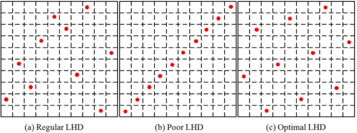
. It is noted that the coordinate of points should be unequal in rows and columns. Figure 5(a) shows a regular LHD with 10 points in 2 dimensions.Latin hypercube designs meet both the space-filling condition and the non-collapsing requirement. It plays an important role in SBGO. Ye and Pan [19] use LHD to produce initial sample points for constructing surrogate models. Viana et al. [73] present a multiple surrogate efficient global optimization algorithm with the help of LHD. The tutorials and reviews on LHD are provided in the literatures [74-76]. 2.2.3. Optimal Latin Hypercube Designs
shown in Figure 5(b) performs the poor space-filling where all points are distributed along the main diagonal. An experimental design with poor space-filling will lead to redundant sample points as well as increasing the computational expense. To extract as more information from the unknown expensive function with minimum number of experimental trails as possible, the promising optimal Latin hypercube designs have been developed depending on a certain optimal criterion like Maximin criterion, i.e. the evaluation points are chosen in such a way that the minimal separation distance among any pair of points is maximized. Other optimal criteria such as Minimax criterion, Entropy criterion, Centered L2 discrepancy criterion are also popularly
used [20]. Obviously, a maximin LHD illustrated in Figure 5(c) is significantly superior than that in Figure 5(a) and Figure 5(b).
OLHD has been widely studied and employed in SBGO. Zhu et al. [77] propose a novel maximin Latin hypercube design using successive local enumeration method. Afterwards, Zhu et al. [40] develop an efficient heuristic surrogate-based global optimization method combining successive local enumeration method and adaptive RBF. Gilkeson et al. [78] present an optimization study of the design of small livestock trailers depending on an optimal LHD. [79] Dong et al. [17] use ESE algorithm to generate optimal experimental points over the entire design space in MSSR.
Figure 5. Latin hypercube designs with 10 points in 2 dimensions.
3. Surrogate Modeling Techniques
After determining a suitable design of experiments method and executing the necessary numerical simulations, the next step is to construct a surrogate model to replace the computationally intensive simulations and analyses model. It can provide a better insight into the expensive black-box optimization problems through visualizing the interactions among objective functions, constraints and design variables as a fast analysis tool. For all surrogate modeling techniques, the relationship between the real response y and the prediction response yɶ is
( ) ( ) ( )
x x xy =yɶ +
ε
(1) where x indicates the design variable,ε
is the approximate error.Various surrogate modeling techniques have been developed for handling the expensive black-box optimization
problems. However, these approaches are appropriate to deal with the different unknown problems due to the different characteristic such as accuracy, efficiency, simplicity, robustness and transparency [23]. An overview of several popularly used surrogate modeling techniques including single surrogate models and ensemble of surrogates is offered. 3.1. Single Surrogate Models
Many alternative single surrogate models exist, here three well-known methods including PRS, RBF and KRG are introduced in this section.
3.1.1. Polynomial Response Surfaces
PRS also called Response Surface Methods (RSM) have been widely used in engineering over several decades. It’s first introduced and further applied by Box and Draper [80]. The general form of PRS model is a polynomial of degree d:
( )
20 , ,...,
i
x i i ij i j ii i ijk i j k i i i id
i j i i i j i k j i
y β β x β x x β x β x x x β x
> > >
= +
∑
+∑∑
+∑
+∑∑∑
+∑
ɶ
(2)
where
β β β β β
0, i, ij, ii, ijk,...,β
i i, ,...,i are the unknowncoefficients, d indicates the order of model. The performance of PRS is largely relying on the value of order d. The high order PRS may probably yield more accurate approximation by allowing more degrees of freedom, but also suffer from the danger of over fitting any noise [11, 81]. In practice, the low order PRS including the first and second order polynomials formulated in Eq. (3) and (4) are commonly used as the
approximate models
( )
0 1x
n
i i i
y
β
β
x=
= +
∑
ɶ (3)
( )
2 10
1 1 1 1
x
n n n n
i i ii i ij i j
i i i j i
y
β
β
xβ
xβ
x x−
= = = = +
= +
∑
+∑
+∑ ∑
where n indicates the number of design variables, the unknown coefficients in Eq. (2), (3) and (4) can be determined by least squares estimation.
Polynomial response surfaces can be simply built, and its smoothing capability allows fast convergence of noisy functions during the search. But, it’s unsuitable for solving the highly nonlinear, high-dimensional or multi-modal problems. Wang [82] presents a global optimization approach combing PRS and inherited LHD to solve the computation-intensive design problems. Vafaeesefat [83] adopt an adaptive PRS to optimize composite pressure vessels with metallic liners. Ye et al. [84] propose a novel surrogate-based optimization method combing PRS and Maxwell finite element for the inductive angle sensor design. Recent advances and applications on PRS are developed in the research [85, 86].
3.1.2. Radial Basis Functions
RBF is originally developed by Hardy [87] for the interpolation of the scattered multivariate data. It has been widely tested and improved since then, meanwhile many significant properties have been obtained. Mullur and Messac [88] propose a more flexible and efficient approximate model: extended radial basis functions combing radial and nonradial basis functions. Gutmann [89] introduces a radial basis functions method to find the global minimum of a continuous nonconvex function. Regis and Shoemaker [90] propose a stochastic radial basis function method for the global optimization of expensive functions. Yao et al. [91] present a novel surrogate-based global optimization approach which integrates a linear interpolation based RBF and a new hybrid infill strategy.
RBF is a linear combinations of a radially symmetric function depending on the Euclidean distance between the sample point and predicted point. Given N points and their real response, the RBF model is formulated as:
( )
(
)
1
x
N
i i
i
y
λ φ
=
=
∑
ɶ x - x (5)
where xi is the vector of design variables at the ith point, λi is the
coefficients of linear combinations, x - xi indicates the
Euclidean distances,φ is a basis function. The most commonly used basis functions include Gaussian, Multiquadric and Cubic, etc. More discussions on RBF can be found in the research by Kitayama et al. [92] and Yao et al. [91].
3.1.3. Kriging
The use of kriging in the context of the modeling and optimization starts with the excellent work by Sacks et al. [93]. It estimates the response values as a combination of a polynomial model plus departures of the form
( )
( ) ( )
1
x x x
m
i i i
y
β
f Z=
=
∑
+ɶ (6)
where βi is the unknown coefficients, fi(x) represents the
known polynomial function that is simply considered to be a
constant in many cases. Z(x) is supposed to be a realization of a random process with mean zero and a nonzero covariance which can be expressed by
( ) ( )
2x ,i xj z ij
Cov Z Z =
σ
R (7) where 2z
σ
is the process variance and Rij is the correlationbetween the ith and jth data points and the relevant correlation function is specified by the user. The introduction of common correlation functions can be found in the paper [94]. The popular Gaussian correlation is formulated as
(
)
(
)
21
x , x exp
n
j
i j i
ij k k k
k
R R θ x x
=
= = − −
∑
(8)where θk indicate the unknown correlation parameters that can
be achieved by maximizing the likelihood of the observed data. More details on KRG can be found in these researches [95-97]. KRG is flexible in capturing nonlinear behaviors due to the correlation functions which can be statistically tuned by the sample data. Moreover, it’s able to provide the estimation of the prediction error. Younis and Dong [98] develop a new SBGO approach called space exploration and unimodal region elimination to speed up the search by using KRG. Moreover, the newly proposed optimization algorithm MSSR utilizes the KRG model to increase search efficiency [17].
3.2. Ensemble of Surrogates
Ensemble of surrogates that combines multiple surrogates via a specific weighting scheme is developed for reducing the prediction uncertainties. The ensemble model is expressed as
( )
( ) ( )
1
x x x
m
e i i
i
y
ω
y=
=
∑
ɶ ɶ (9)
where m is the number of individual surrogates, yɶe
( )
xindicates the predicted response by the ensemble of surrogates,
( )
xi
yɶ and
ω
i( )
x denote the predicted response and thecorresponding weight factor of the ith surrogate, separately. Generally, the weights are smaller as the corresponding surrogates are less accurate and vice versa. For improving the overall accuracy, a variety of wise methods allocating different weights to different single surrogates have attracted plenty of attention. In this section, several noteworthy ensemble of surrogates about weights selection procedures proposed by various researchers are introduced in the order of their publications.
3.2.1. Heuristic Computation of the Weights
these two issues, Goel et al. [31] propose a heuristic approach to calculate the weights using Prediction Sum of Squares
(PRESS), which is formulated as follows:
(
)
* * *
1 1
1
, , , 1 0
m m
i i j i i i
j i
E E E E
m
β
ω ω
ω ω
α
α
β
= =
=
∑
= + =∑
< < (10)where Ei indicates the PRESS of the ith surrogate computed
from
( )
( )
(
( ))
21
1
= x x
N
k
i k i k
k
E y y
N
−
=
−
∑
ɶ (11)where N is the amount of training points, xk is the kth sample
point, y(xk) indicates the actual response value at xk and
( )
( )
x
k
i k
yɶ − represents the predicted response of the ith
surrogate model built using N-1 training points without the kth
point at xk (i.e., leave one out cross validation strategy). This
parameters α and β are defined to separately control the importance of averaging and individual surrogate. Large values of α and small negative values of β represent the high confidence in the averaging scheme, while small values of α
and large negative values of β reflect high weights to the best surrogate model.
Goel et al. [31] suggest that α = 0.05 and β = -1 are better for most cases in their research. Nevertheless, the fixed values of these two parameters can not be available for all problems. On the contrary, the freedom of determining the parameters α and
β provides the weighting selection method more flexibility. Acar and Rais-Rohani [32] recommend that two parameters α
and β can be optimized for minimizing a certain global error metric of the ensemble. Motivated by this idea, the selection of weights is also treated as an optimization problem to minimize PRESS with a strict constraint by Ye and Pan [19].
3.2.2. Weights Selection Based on Local Error Metric Sanchez et al. [99] consider that using a local error metric may obtain more accurate predictions by allowing flexible weights over the whole design space than the use of a global error measure. A new ensemble of kernel-based surrogates under the alternative loss functions with weights based on the empirically estimated prediction variances is presented. The prediction variance is used as the local error metric. Meanwhile, the value of weight factor for individual surrogate model is set to be inversely proportional to an estimation of the prediction variance as
( )
( )
( )
2 2 1 1 x x 1 x i i m j jσ
ω
σ
= =∑
(12)where x indicates the prediction point, m is the amount of surrogate models, 2
( )
x
i
σ represents the prediction variance of the ith surrogate model which are calculated from the v
nearest neighbors of the prediction point x. This empirical formula is given as
( )
(
( )
( )
)
22 1 1 x = 1 v
i h i h
h
y s y s
v
-σ
=
−
∑
ɶ (13)where s1, s2,..., sv mean the v nearest neighbors of the point x
whose relevant real response and predicted response values of the ith surrogate model are y(s1), y(s2),..., y(sv) and y sɶi
( )
1 ,( )
2 , ,( )
i i v
y sɶ
⋯
y sɶ , respectively. Here, v=3 is advised bySanchez et al. [99].
3.2.3. Weights Selection Based on Minimizing MSE
Motivated by the work of Bishop [100], Acar and Rais-Rohani [32], Viana et al. [101] develop a new weights selection method by using minimizing Mean Square Error (MSE) as
( )
2
1
MSEen en x x ω CωT
Ve d V
=
∫
= (14)where
( ) ( )
x x( )
xen
e =y −yɶen means the prediction error of
ensemble of surrogates. The integral taken over the domain of interest allows the computation of the elements in C
( ) ( )
1x x x
ij i j
V
c e e d
V
=
∫
(15)where ei (x) and ej (x) represent the prediction errors of the ith
and jth surrogate models, separately.
The matrix C in Eq. (14) plays the same role as the covariance matrix in Bishop’s formulation. Here, it’s approximated by the use of the vectors of cross validation errors eɶ. Thus, the formulation of Eq. (15) will be modified as
1 e eT
ij i j c
N
= ɶ ɶ (16)
Given matrix C, the optimal values of weights can be achieved by minimizing MSE as
ω
min MSE ω Cω
. . 1 ω 1
T en
T s t
=
= (17)
The weight factors can be obtained by utilizing Lagrange multipliers as
1
1
C 1 ω
1 C 1T
− −
= (18)
whose meaning is unable to explain in real-world applications. Viana et al. [101] consider that this disadvantage will amplify the errors generating from the approximation of elements in matrix C and advise to solve Eq. (18) using only the diagonal elements in matrix C which are more accurate than the off-diagonal terms.
4. Infill Criteria
In general, SBGO can be categorized as one-stage and two-stage methods [81]. In the one-stage method, sample points are generated all at once, and then the interpolation of the response surface as well as the determination of the global optimum are completed in the same calculations. As no a priori knowledge about the black-box problem is available, it mainly leads to a waste of computational resources. Furthermore, it’s hard for researchers to determine the appropriate sample size beforehand. Different from the one-stage method, the two-stage method is more significant, tractable and attractive. The surrogate models are first built with the initial training points generated by DOE. Afterwards, new points are obtained over the design space using the infill criteria also named as adaptive designs or sequential designs [35]. The procedure is repeated until a convergence criterion or a termination criterion like the maximum number of function evaluations allowed is reached. The new points which are used to sequentially update the surrogate models and increase the probability of identifying the global minimum are evaluated from the expensive models, not that from the cheap surrogate models. One hand, this two-stage method can extract useful information from the approximate models and speed up the optimization process. On the other hand, it allows designers to stop the optimization process as soon as the satisfactory optimal solution is achieved [102]. The adaptive designs have gained popularity in recent years compared to the one-stage method. In this section, infill criteria are discussed.
Infill criteria guide how new points are generated to support the surrogate modeling, design optimization and applications. The candidate points are obtained by sufficiently utilizing the information from the current optimization process. These supplementary points can offer much more information on the expensive black-box problem, and the more points we own,
the more we know about the black-box problem. Infill criteria are generally employed for both surrogate modeling and surrogate-based global optimization. For surrogate modeling, it concentrates on continuously improving the accuracy of surrogate models. Moreover, it focuses on searching the global optimum for surrogate-based global optimization.
Infill criteria can be also classified as exploitation and exploration as same as SBGO. The exploitation strategy directly takes the surrogate model replace the actual model as the objective function and considers the current optimal points as the new supplementary points. This pure exploitation strategy will rapidly converge to an optimal solution of the surrogate surface whereas it can’t be guaranteed to find the actual global optimum. In fact, only the sequential augment of optimal points may lead to the local optimum due to the lack of exploration [103]. On the contrary, the pure exploration strategy explores the unvisited or sparse regions for enhancing the global approximation and avoiding falling into the local optimum. However, it will be a waste of computational time to blindly enhance the global accuracy while the global optimum itself is just required. Only high accuracy in the potentially promising regions is required for SBGO.
There are two requirements for surrogate-based global optimization that have to be satisfied: exploitation of the promising candidates and exploration of the sparse regions. The target is to identify the near global optimum and avoid missing the true global optimum within an affordable computational cost. In practice, infill criteria have a significant influence on efficiently and accurately locating the global optimum. Therefore, the infill criteria which combine exploitation and exploration strategy to balance their competing goals have been widely studied and advanced [91, 92, 104]. Next, some representative infill criteria intended to promote exploration and exploitation are reviewed
Jones et al. [34] develop a famous infill criterion named Expected Improvement (EI) which has been manipulated by many researchers for Gaussian process based global optimization. Additional points which have either high uncertainty or low objective function values are selected by EI. It can balance the requirements to exploit the approximate model with the need to improve the global approximation. This EI criterion is given as below
( )
(
min( )
)
min( )
( )
( )
min( )
( )
x x
x Φ x , 0
x x x
0 0
y y y y
y y s if s
E I s s
if s
φ
− −
− + >
=
=
ɶ ɶ
ɶ
,
(19)
where ymin indicates the best point found so far, yɶ
( )
x meansthe predicated response at point x, Φ and φ represent the cumulative distribution and probability density function, separately. s2(x) indicates the estimated MSE of the surrogate model, which is formulated as
( )
(
)
2 1
2 2 1
1
1 Ψ ψ
x 1 ψ Ψ ψ +
Ψ T T
T
s σ
− −
−
−
= −
1
1 1 (20)
where
σ
is the covariance, ψ indicates the vector of correlation between the prediction data and observed data, Ψ represents the correlation matrix for all observed data provided by KRG correlation function.In EI criterion, the term ymin
-
yɶ( )
x indicates the amountinfill criterion for seeking the global optimum from a number of publications. Many modified EI including generalized expected improvement [105], weighted expected improvement [36] and quantile-based expected improvement [106] have shown well generality and performance for various engineering applications. Further studies have adapted EI to generate multiple update points, not a single point. Ginsbourger et al. [107] propose a multi-points expected improvement to take advantage of parallel computation facilities. Viana et al. select multi points at each iteration with the aid of expected improvement. Generating multiple points per optimization cycle and allowing distribution of the expensive function evaluations on several processors provides a large potential to accelerate the search process.
Kitayama et al. [92] consider that it is important to simultaneously add the new sample points around: a) the optimum of the response surface and, b) the sparse region in the design space. Thus, they propose a new infill criterion that adding the optimal point of response surface in each cycle as the new sample point to meet the first objective and taking the global optimum of the density function as another additional point to satisfy the second objective. The aim of the density function is to discover a sparse region. It is expected that the addition of new sample points in the sparse region will lead to global approximation. The density function is applied to improve the accuracy of surrogates by Kitayama et al. [103] and Ye et al. [108]. Gu et al. [104] develop a new and adaptive sampling mechanism which selects new sample data adaptively based on the values evaluated by three well-known surrogate modeling techniques concurrently to improve the overall accuracy of the hybrid model and the efficiency of the global search. This infill criterion is widely adopted for SBGO [19, 109]. In addition, other heuristic infill criteria have also been investigated. Wang et al. [39] introduce a novel infill criterion that sample points with low values and high values, but have a non-zero probability are both preferred. Villanueva et al. [110] choose new points in the mall subspace which are partitioned by clustering method. Meanwhile, some optimal points are also selected to improve the local approximation. Dong et al. [17] take local optima of response surfaces for exploitation and use the estimated MSE to explore the unknown areas using KRG and design space reduction method. Müller and Shoemaker [111] introduce a random sampling strategy and a strategy where the minimum point of the response surface is used as new sample point for computationally expensive black-box global optimization problems. Amine et al. [112] propose a new infill criterion that incorporates minimizing the surrogate model while also maximizing the expected improvement criterion for high-dimensional constrained problems.
5. Design Space Reduction
A prominent challenge arises in surrogate-based global optimization while the expensive black- box system involves a large amount of design variables and a large size of design space. Despite the improved optimization algorithms and the advanced computation power, the continuously increased calculation burden still becomes a great challenge to the solution of the large-scale problem. The number of expensive function evaluations required to explore the design space is normally exponential to the number of input variables and the size of input spaces. For instance, considering an engineering design optimization problem involving 10 input variables whose bounds are both [0, 1]. If an interval value 0.5 is used for each variable, a design of experiments with 310 samples that means plenty of expensive simulations are needed. Therefore, as an efficient branch to alleviate this challenge, the design space reduction method has been widely studied recently. Generally, two kinds of design space reduction schemes exist in the correlative literatures. The first strategy seeks to decrease the dimensionality of the design space through removing the unimportant variables. Another strategy is employed to reduce the size of the design space through identifying the small promising sub-region. Next, these two design space reduction methods are introduced in detail. 5.1. Dimensionality Reduction Methods
It’s known to all that the curse of dimensionality is a phenomenon as the design variables are so large that it may challenges numerical analysis technologies and optimum seeking technologies. Thus, regular methods are doomed to failure for solving the high-dimensional problems. An active method to deal with the high-dimensional spaces is to select smaller number of variables in place of the real variables known as dimensionality reduction. Dimensionality reduction methods have been increasingly employed in the fields of complex high-dimensional design problems as it can maximally keep the important features and eliminate the less significant or insignificant.
As a dimensionality reduction method, global sensitivity analysis has been popularly applied for engineering design optimization. It can well compare the relative magnitude of the impact on each design variable on the output because the significant input variables possess the larger design sensitivity. Design variables with smaller sensitivity are identified and removed to decrease the number of design variables. To understand the concept, assume a square integrable objective function approximated by a surrogate model whose values are scaled between zero and one. It can be decomposed into summands of increasing dimensionality as [11]
( )
x 0 i( )
i ij(
i, j)
1,2, ,n(
1, 2, , n)
i i j
f f f x f x x f x x x
<
= +
∑
+∑
+ +⋯ ⋯ ⋯ (21)where n is the amount of design parameters, f0 indicates the
zeroth order component function which indicates the mean effect to f(x). Likewise, fi(xi), fij(xi, xj) and f1, 2,..., n(x1, x2,..., xn)
represent the first order, second order and nth order effects to f
( )
(
)
1 1 1 1
2 2
0
2
, , , ,
= x x
= , , , ,
s s s s
i i i i i i i i
D f d f
D f x x dx x
−
∫
∫
⋯ ⋯ ⋯ ⋯
(22)
The partial variances provide a measure of the contribution of each individual parameter. Moreover, the total variance is a sum of partial variances of the independent parameters and combinations of parameters.
The individual sensitivity index which indicates the impact of an input variable to a function variability is expressed as
1, ,s= 1, ,s i i i i
S ⋯ D ⋯ D (23)
Indexs
1, ,s i i
S ⋯ contain first order and higher order indices that offer the effect of individual variable and other possible mixed influence of various variables [113]. The relative importance of a certain input variable can also be quantified by the total sensitivity index except individual sensitivity index whereas the total sensitivity index for the ith input variable is defined as the sum of all partial sensitivity indices involving parameter i, divided by the total variance as
(
)
{
}
1, , 1, ,
1
,
, , : ,1 ,
s s
i T
i i i i
i s k
S D
i i k k s i i
ϑ
ϑ
=
= ∃ ≤ ≤ =
∑
⋯ ⋯
⋯
(24)
The detail introduction can be found in the literature [113]. The individual sensitivity index refers to the fraction of the total variance, while the total sensitivity index indicates the contribution of all partial variance.
The relative importance of each design variable can be observed by comparing either their individual sensitivity index or total sensitivity index. In addition, the difference between the individual sensitivity and total sensitivity for each variable also provides an indication of the degree of interaction among variables. The design variables with less importance and interaction can be removed to reduce the computational cost. Fu et al. [114] investigate the use of global sensitivity analysis as a screening tool for reducing the computational burden for rehabilitation of water distribution systems. Marrel et al. [115] use the global sensitivity analysis to quantify the effect of uncertain design parameters on the variability in stochastic computer models with joint metamodels. Recent advances on various global sensitivity analysis approaches are provided by Iooss and Lemaître [116]. It’s noted that the history of using dimensionality reduction in design optimization can trace back to several decades ago. Dimensionality reduction methods like global sensitivity analysis, Principal Component Analysis (PCA), Analysis of Variances (ANOVA) and mapping etc., have long been used in various science and engineering disciplines as a preprocessing step for handling high-dimensional data. PCA can transform data to a new coordinate system by data projection so that the design variables with greatest variances in the projection come to the principal coordinates. Raghavan et al. [117] use PCA and diffuse approximation method in place of the
geometry-based variables with the smallest set of variables originally required for structural shape optimization. ANOVA is a collection of statistical models applied to analyze the differences among groups and their associated procedures. Zhang et al. [118] develop an efficient ANOVA-based stochastic circuit systems simulator to avoid the curse of dimensionality. For reducing the amount of dimensions, mapping transforms a group of correlated parameters into a smaller group of new uncorrelated parameters for retaining most of the primary information. Qiu et al. [119] propose a multi-stage design space reduction method using the fuzzy clustering strategy and mapping technology to improve the modeling accuracy and optimization efficiency. Furthermore, Shan and Wang [43] introduce some strategies for tackling the difficulties caused by high dimensionality.
5.2. Size Reduction Methods
Despite the dimensionality reduction methods have been tried to enhance capability of SBGO for computation-intensive high-dimensional optimization problems, it’s still rather hard to precisely identify the insignificant variables, especially for MOO and MDO problems. Alternatively, more and more researchers turn to reduce the size of design space while the dimensionality is difficult to reduce. At the first stage of defining a real-word application, researchers are used to offer very conservative upper and lower bounds for design variables due to the lack of sufficient knowledge on the function behavior and interactions between the objective and constraint functions. The combined range of each variable dictates the size of design space and a broad range of input variables results in a large size of design space, limiting the application of SBGO, greatly.
Size reduction means shrinking a design space so that the focus of modeling can be in a small attractive region. A common size reduction method begins with generating a smaller amount of points and its response surface values. Then the size of design space is adaptively changed depending on the feedback information from these known expensive points. Thus, the efficiency of finding and quality of the global optimum will be increased by exploring an interested subspace. In the context of this kind of design space reduction, several methods have been reported. Among them, FCM has been diffusely used in many publications. Given the number of cluster c, the overall dissimilarity between each cluster center and each data point can be given as
(
)
( )
[ ]
t 2
1 1
1
,
. . 1, 0,1
N c
ct ik k i
k i c
ik ik i
J U u x v
s t u u
= =
=
= −
= ∈
∑∑
∑
v
(25)
where U is the fuzzy c-partition matrix of N data points xk (k=
1, 2…, N, x ∈ ), v = (v1, v2,…, vc), vi is the ith cluster center, 1
≤ i ≤ c, t is a constant greater than 1 (typically t=2), uik is the
space due to its robustness, convenience and simplicity. Wang et al. [120] present a surrogate-based optimization method using multi-level fuzzy clustering space reduction strategy with KRG interpolation for expensive black-box optimization problems. Ye and Pan [41] propose an ensemble of surrogate-based optimization method integrating with FCM to deal with the computation-intensive, black-box optimization problems. Shi et al. [121] introduce a new approximate optimization method that uses RBF to approximate the expensive simulations in an interesting subspace obtained by FCM method for improving the efficiency and convergence.
Many size reduction methods like rough set and trust region are also frequently used in design optimization, except fuzzy clustering methods. Rough set theory seeking to synthesize approximation of concepts from the acquired data is developed by Pawlak [122] in the early 1980s. Shan and Wang [123] first introduce the rough set into the mechanical design area to systematically identify attractive reduced regions. Chu et al. [124] develop an expert system using rough set theory and self-organizing maps to guide researchers to partition and reduce the design space. Trust region is a term used in mathematical optimization to denote the subset of the region of the objective function. Farias et al. [125] introduce a trust region based framework employed to adaptively update the design space to solve optimization problems of fluid-structure interaction. Ollar et al. [126] present a novel method to solve multidisciplinary design optimization problems using approximations built in subspaces obtained by trust region. Eason [127] propose a novel trust region filter algorithm for black box optimization, which is both robust to lack of derivatives in some constraints while also taking advantage of equation oriented constraints. Conn et al. [128] address trust-region methods for unconstrained derivative-free optimization. These methods maintain linear or quadratic models which are based only on the objective function values computed at sample points. Wild and Shoemaker [129] introduce and analyze the first-order derivative-free trust-region algorithms based on RBF, which are globally convergent. Gratton and Vicente [130] present a surrogate management framework using rigorous trust-region steps.
6. Future Challenges and Research
Though extensive and intensive research on surrogate modeling and surrogate-based global optimization has been implemented and achieved considerable advances over the past decade, some major challenges remain to be addressed. Challenges of expensive black-box optimization problems come from several main aspects: (1) large-scale problems, which imply a huge number of design variables or a large size of design spaces, (2) unknown function characteristics, that mean no prior information about the characteristics of the black-box functions, (3) intelligent sampling designs, that signify a minimum number of sample points intelligently generated to describe the black-box function, and (4) various optimization needs, which contain dynamic optimization,
combinatorial optimization, probabilistic optimization, multi-objective optimization and so on. Following future challenges and research directions are discussed to trigger more promising efforts.
6.1. Large-Scale Problems
It’s basically recognized that the total high computation expense for large-scale problems makes the SBGO methods less attractive or even impractical. Much work should be carried out while large-scale problems have just gotten more complex. However, there seems to be a lack of research on large-scale problems and a lot of difficulties or challenges haven’t been worked out. For instance, which kind of surrogate models or sampling designs best fit the large-scale problems. Moreover, what strategies can efficiently facilitate the optimization process and further increase efficiency. Is the design space reduction approaches always work? It is expected that SBGO methods can be expediently adapted to more complicated large-scale optimization problems and obtain more benefits in improving computational accuracy and optimization efficiency.
Although a mass of design space reduction methods contribute to identify smaller promising regions, a variety of excellent approaches or techniques are required to face with this large-scale challenge. For example, surrogate modeling techniques used at present like PRS, RBF and KRG are all unsatisfactory for large-scale problems and various model types are needed, especially for large-scale problems. Furthermore, parallel computing techniques can also be used to decompose the main computation task into independent tasks at each iteration for speeding up the algorithms.
6.2. Unknown Functions Characteristics
In order to precisely approximate the expensive black-box problems, a deep understanding of the unknown functions is felt necessary. Nevertheless, the characteristics are unknown for most of engineering design optimization problems. For instance, what are the characteristics of a large-scale problem? Recent researches turn to focus on developing more flexible and generic SBGO methods. Many types of surrogate modeling techniques including multi-level, variable fidelity and ensemble of surrogates etc., have been employed to increase the overall performance. It offers a more efficient way for researchers with no need for deep knowledge on surrogate modeling techniques and sampling designs as well as the prior information on characteristics of the unknown functions.
6.3. Intelligent Sampling Designs
Current sampling schemes for SBGO methods concentrate on the initial sampling designs and adaptive sampling designs for purpose of achieving certain sample points. On the one hand, initial sampling designs mainly seek for the points with both good projective properties and space filling properties. However, it’s difficult to meet these two requirements for high-dimensional problems. For example, LHD suffers from the curse of dimensionality as any other space-filling DOE that the sample normally creates a vacuum in the center of design space while uniformity in each dimension is preserved. Besides, the best initial sampling size remains to be a mystery that has a large effect on the efficiency and accuracy of surrogate modeling process. The distribution of the initial sample points becomes less important without knowing the best sampling size. On the other hand, the adaptive sampling designs have gradually displaced the initial sampling designs in terms of reflecting the black-box function characteristics. Though there are lots of approaches on adaptive sampling designs as reported before, more intelligent sampling designs are required to further improve the SBGO methods.
6.4. Various Optimization Needs
Various optimization needs including multi-objective optimization for meeting multiple design objectives, probabilistic optimization when uncertainties of design variables are considered, dynamic optimization which is time-varying, and multidisciplinary design optimization where coupling between different disciplines is present have their own challenges, combinatorial optimization where the discrete variables are considered, stochastic optimization where the input information into the optimization method may be contaminated with noise. Therefore, the subtle differences between each type of optimization needs should deserve enough attention. There is much work to do in spite of various SBGO methods have been intensively applied to deal with various optimization needs involve expensive computation. In the case of dynamic optimization, the surrogate models must be updated online. It may be beneficial to introduce incremental online learning techniques for dynamic optimization. Therefore, new innovative SBGO methods should be created to satisfy various optimization needs in the future.
7. Conclusions
This paper provides an overview of recent advances in surrogate-based global optimization methods for expensive black-box problems. Research and advancement in SBGO are divided into five topics depending on the role of surrogate modeling techniques in supporting design optimization, including design of experiments, surrogate modeling techniques, infill criteria and design space reduction. Future challenges and research are also discussed. The primary issues reviewed are summarized as follows:
Design of experiments including three typical designs of physical experiments methods and three well-known design of computer experiments methods are introduced.
Surrogate modeling techniques containing three representative single surrogate models containing PRS, RBF, KRG, and three popular ensembles of surrogates are presented.
Infill criteria which guide to generate new sample points for continuously improving the accuracy of surrogate models are discussed.
Design space reduction that can be generally categorized into two types: dimensionality reduction methods and size reduction methods are reviewed.
Future challenges and research on four main aspects including large-scale problems, unknown function characteristics, intelligent sampling designs and various optimization needs are discussed
SBGO is an active area of research and has made substantial progress in handling engineering design optimization problems. It’s hoped that this work can help new engineers and researchers who are just beginning in this field. Meanwhile, it’s also expected that this work will help experienced engineers and researchers as a reference or inspiration for future work.
Conflict of Interests
The authors declare that they have no competing interests.
Funding
This research was funded by the National Natural Science Foundation of China under Grant No. 61803306, 51709229, 51879220, 51979226, the National Key Research and Development Project of China under Grant No. 2016YFC0301300, and the Fundamental Research Funds for the Central Universities under Grant No. 3102019HHZY03009.
References
[1] Younis A, Dong Z (2010) Trends, features, and tests of common and recently introduced global optimization methods. Engineering Optimization 42 (8): 1-28.
[2] Rios LM, Sahinidis NV (2013) Derivative-free optimization: a review of algorithms and comparison of software implementations. Journal of Global Optimization 56 (3): 1247-1293.
[3] Xiao YY, Zhao QH, Kaku I et al. (2014) Variable neighbourhood simulated annealing algorithm for capacitated vehicle routing problems. Engineering Optimization 46 (4): 562-579.
[5] Lu L, Gao Y, Li Q et al. (2018) Numerical investigations of tip clearance flow characteristics of a pumpjet propulsor. International Journal of Naval Architecture and Ocean Engineering 10 (3): 307-317.
[6] Younis A, Karakoc K, Dong Z et al. (2011) Application of SEUMRE global optimization algorithm in automotive magnetorheological brake design. Structural and Multidisciplinary Optimization 44 (6): 761-772.
[7] Sun C, Song B, Wang P (2015) Parametric geometric model and shape optimization of an underwater glider with blended-wing-body. International Journal of Naval Architecture and Ocean Engineering 7 (6): 995-1006.
[8] Lee H, Jo Y, Lee DJ et al. (2016) Surrogate model based design optimization of multiple wing sails considering flow interaction effect. Ocean Engineering 121: 422-436.
[9] Mainini L, Willcox K (2015) Surrogate modeling approach to support real-time structural assessment and decision making. AIAA Journal 53 (6): 1612-1626.
[10] Peherstorfer B, Kramer B, Willcox K (2017) Combining multiple surrogate models to accelerate failure probability estimation with expensive high-fidelity models. Journal of Computational Physics 341: 61-75.
[11] Shyy W, Cho YC, Du W et al. (2011) Surrogate-based modeling and dimension reduction techniques for multi-scale mechanics problems. Acta Mechanica Sinica 27 (6): 845-865. [12] Wang GG, Shan S (2007) Review of metamodeling techniques
in support of engineering design optimization. Journal of Mechanical design 129 (4): 370-380.
[13] El-Taweel T, Haridy S (2014)