A CUDA-based GPU engine for gprMax: open source
FDTD electromagnetic simulation software
Craig Warrena,∗, Antonios Giannopoulosb, Alan Grayc, Iraklis Giannakisb, Alan Pattersond, Laura Wetterd, Andre Hamrahd
aDepartment of Mechanical & Construction Engineering, Northumbria University,
Newcastle upon Tyne NE1 8ST, UK
bSchool of Engineering, The University of Edinburgh, Edinburgh EH9 3JL, UK
cNVIDIA, UK
dGoogle, USA
Abstract
The Finite-Difference Time-Domain (FDTD) method is a popular numeri-cal modelling technique in computational electromagnetics. The volumetric nature of the FDTD technique means simulations often require extensive computational resources (both processing time and memory). The simula-tion of Ground Penetrating Radar (GPR) is one such challenge, where the GPR transducer, subsurface/structure, and targets must all be included in the model, and must all be adequately discretised. Additionally, forward sim-ulations of GPR can necessitate hundreds of models with different geometries (A-scans) to be executed. This is exacerbated by an order of magnitude when solving the inverse GPR problem or when using forward models to train ma-chine learning algorithms.
We have developed one of the first open source GPU-accelerated FDTD solvers specifically focussed on modelling GPR. We designed optimal ker-nels for GPU execution using NVIDIA’s CUDA framework. Our GPU solver achieved performance throughputs of up to 1194 Mcells/s and 3405 Mcells/s on NVIDIA Kepler and Pascal architectures, respectively. This is up to 30 times faster than the parallelised (OpenMP) CPU solver can achieve on a commonly-used desktop CPU (Intel Core i7-4790K). We found the cost-performance benefit of the NVIDIA GeForce-series Pascal-based GPUs –
∗Corresponding author.
E-mail address: [email protected]
targeted towards the gaming market – to be especially notable, potentially allowing many individuals to benefit from this work using commodity work-stations. We also note that the equivalent Tesla-series P100 GPU – targeted towards data-centre usage – demonstrates significant overall performance ad-vantages due to its use of high-bandwidth memory. The performance benefits of our GPU-accelerated solver were demonstrated in a GPR environment by running a large-scale, realistic (including dispersive media, rough surface to-pography, and detailed antenna model) simulation of a buried anti-personnel landmine scenario.
Keywords: CUDA, Finite-Difference Time-Domain, GPR, GPGPU, GPU, NVIDIA
NEW VERSION PROGRAM SUMMARY Program Title: gprMax
Licensing provisions: GPLv3
Programming language: Python, Cython, CUDA
Journal reference of previous version: http://dx.doi.org/10.1016/j.cpc. 2016.08.020
Does the new version supersede the previous version?: Yes
Reasons for the new version: Performance improvements due to implementation of CUDA-based GPU engine
Summary of revisions: A FDTD solver has been written in CUDA for execution on NVIDIA GPUs. This is in addition to the existing FDTD solver which has been parallelised using Cython/OpenMP for running on CPUs.
Nature of problem: Classical electrodynamics
Solution method: Finite-Difference Time-Domain (FDTD)
1. Introduction
only accessible to those working in universities, big businesses, or national research centres. Over the past decade general-purpose computing using graphics processing units (GPGPU) has become a common method for ac-celerating scientific software. GPGPU is attractive because a GPU has a massively parallel architecture, typically consisting of thousands of efficient cores designed for handling specific tasks simultaneously. In contrast, a CPU has few cores that are designed to handle more generic sequential tasks. Combined with the relatively low cost of GPUs, it makes GPGPU appealing from a cost-performance perspective – from small-scale workstation setups through to large-scale GPU-accelerated HPC facilities. In addition, the cre-ation of programming environments such as CUDA [1], available for NVIDIA GPUs, have made GPGPU computing more accessible to developers without necessitating expertise in computer graphics.
In the field of computational electromagnetics (EM), the Finite-Difference Time-Domain (FDTD) method is one of the most popular numerical tech-niques for solving EM wave propagation problems. One such set of problems is the simulation of Ground Penetrating Radar (GPR), where the GPR trans-ducer, subsurface/structure, and targets must all be included in the model. GPR antennas are typically impulse-driven and broadband, so the time-domain nature of the FDTD method means this behaviour can be modelled with a single simulation, i.e. separate simulations are not required for each excitation frequency. In general the strengths of the FDTD method are that it is fully explicit, versatile, robust, and relatively simple to implement. How-ever, it can suffer from errors due to ’stair-case’ approximations of complex geometrical details, and the aforementioned requirement – to discretise the entire computational domain – can also be disadvantageous in necessitating extensive computational resources. The building block of the FDTD method is the Yee cell [2] in which Maxwell’s curl equations are discretised in space and time (usually using second-order accurate derivatives). A leapfrog time-stepping method is used to alternately update the three electric and three magnetic field components in three-dimensional (3D) space. At each time-step the electric and magnetic field updates are performed independently at each point of the computational grid. This grid-based parallelism can be mapped to multiple computational threads running in parallel. This has led to both commercial and open source FDTD EM software being paral-lelised for CPU solving [3, 4, 5, 6, 7, 8] and, more recently, some commercial codes being accelerated using GPGPU. However, there are currently no open source FDTD EM tools that are GPU-accelerated and contain the necessary
features to simulate complex, heterogeneous GPR environments. There is a clear need for such tools in areas of GPR research such as full-waveform inversion [9, 10] and machine learning [11], where thousands of complex and realistic forward models required to be executed.
We have developed a GPU-accelerated FDTD solver and integrated it into open source EM simulation software that is specifically focussed on modelling GPR. In Section 2 we explain the design of the GPU kernels and optimisa-tions that have been employed. Section 3 presents performance comparisons, using simple models, between the existing parallelised CPU solver and our new GPU solver, on a selection of NVIDIA GPUs. In Section 4 we demon-strate the performance of the GPU-accelerated solver with a more represen-tative, realistic GPR simulation, as well as with a large-scale GPR simulation of buried anti-personnel landmines. Finally, Section 5 gives our conclusions.
2. Kernel design
A GPU-accelerated FDTD solver has been developed as an integral com-ponent of gprMax1 which is open source software that simulates electromag-netic wave propagation, using the FDTD method, for numerical modelling of GPR. gprMax is one of the most widely used simulation tools in the GPR community, and has been successfully used for a diverse range of applica-tions in academia and industry [12, 13, 14, 15, 16, 17]. It has recently been completely re-written [18] in Python with the CPU solver component writ-ten in Cython2 and parallelised using OpenMP. This recent work [18] also introduced a unique combination of advanced features for simulating GPR including: modelling of dispersive media using multi-pole Debye, Drude or Lorenz expressions [19]; soil modelling using a semi-empirical formulation for dielectric properties and fractals for geometric characteristics [20]; diagonally anisotropic materials; rough surface generation; an unsplit implementation of higher order perfectly matched layers (PMLs) using a recursive integration approach [21]; and the ability to embed complex transducers [22] and targets. As previously stated one of the reasons the FDTD method is attractive to parallelise is because at each time-step the electric and magnetic field updates can be performed independently at each point of the computational
grid. A standard FDTD update equation (omitting the source term) for the electric field component in the x-direction (Ex) is given by (1) [23].
Ex
n+12
i,j+12,k+12
=Ca,Ex
i,j+1
2,k+ 1 2 Ex
n−1 2
i,j+12,k+12 +Cbz,Ex
i,j+1
2,k+ 1 2 Hz n
i,j+1,k+12
−Hz
n
i,j,k+12
!
−Cby,Ex
i,j+1
2,k+ 1 2 Hy n
i,j+12,k+1
−Hy
n
i,j+12,k
!
,
(1)
where Ca and Cb are the coefficients related to the material properties, Hy and Hz are the magnetic field components in the y- and z-directions, the superscript n denotes the time-step, and the subscripts (i, j, k) denote the 3D spatial location. It is evident from (1) that updatingEx is a fully explicit operation, i.e. it depends only on quantities stored in memory from previous time-steps.
GPUs offer performance advantages over traditional CPUs because they have significantly higher computational floating point performance (through many lightweight cores) coupled with a relatively high bandwidth memory system. The roofline model [24] can be used to determine which of these aspects is the limiting factor, given the ratio of operations to bytes loaded, for any given algorithm. In (1) a total of six field components (electric or magnetic) are either loaded or stored, corresponding to 24 or 48 bytes of data in single or double precision. Seven floating point operations are performed so the ratio is 0.3 (single precision) or 0.15 (double precision), which is much less than the equivalent ratio offered by the hardware (called the “ridge point” in the roofline model terminology). This tells us that the code will not be sensitive to floating point capability, and that the available memory bandwidth will dictate the performance of our algorithm.
Listing 1 shows an example of one of our kernels for updating the elec-tric field for non-dispersive materials. There are several important design decisions and optimisations that we have made with the kernel:
• We use one-dimensional (1D) indexing for defining the number of blocks in a grid, and the number of threads in a block. We want to make cer-tain we achieve memory coalescing by ensuring that consecutive threads access consecutive memory locations. This is demonstrated in Listing 1 as kis the fastest moving thread index, and consecutive ks correspond
to consecutive elements of Ex. We are aware of other implementations for domadecomposition using two-dimensional planes or fully 3D in-dexing [25, 26, 27]. However, we found 1D inin-dexing offered simpler implementation, similar performance, and more flexibility in terms of different domain sizes that might be encountered.
• We define macros within all the GPU kernels to convert from traditional 3D subscripts (i, j, k) to linear indices that are required to access ar-rays in GPU memory. The macros are principally used to maintain readability, i.e. both CPU and GPU codes closely resemble the tradi-tional presentation of the FDTD algorithm. If linear indices had been used directly the kernel would be much less readable and would differ from the CPU solver which uses traditional 3D subscripts to access 3D arrays. This design choice takes on further significance for the more complex kernels, such as those used to update the electric and mag-netic field components for materials with multi-pole Debye, Lorenz, or Drude dispersion, or those used to update the PML.
• We make use of the constant memory (64KB), available through CUDA, on NVIDIA GPUs. Constant memory is cached, so normally costs only a read from cache which is much faster than a read from global mem-ory. Electric and magnetic material coefficients, i.e. Ca and Cb from (1), for materials in a model are stored in constant memory.
• We mark pointers to arrays which will be read-only with theconst and restrict qualifiers. This increases the likely-hood that the compiler will detect the read-only condition, and can therefore make use of the texture cache – a special on-chip resource designed to allow efficient read-only access from global memory.
• Finally, we include the functions to update all the electric field com-ponents, Ex, Ey, and Ez3, in a single kernel, to benefit from kernel caching.
3For the sake of brevity only the function for updating theE
// Macros for converting subscripts to linear index:
#define INDEX2D_MAT(m, n) (m)*(£NY_MATCOEFFS)+(n) #define INDEX3D_FIELDS(i, j, k)
(i)*(£NY_FIELDS)*(£NZ_FIELDS)+(j)*(£NZ_FIELDS)+(k)
,→
#define INDEX4D_ID(p, i, j, k)
(p)*(£NX_ID)*(£NY_ID)*(£NZ_ID)+(i)*(£NY_ID)*(£NZ_ID)+(j)*(£NZ_ID)+(k)
,→
// Material coefficients (read-only) in constant memory (64KB)
__device__ __constant__ $REAL updatecoeffsE[$N_updatecoeffsE];
__global__ void update_e(int NX, int NY, int NZ, const unsigned int*
__restrict__ ID, $REAL *Ex, $REAL *Ey, $REAL *Ez, const $REAL*
__restrict__ Hx, const $REAL* __restrict__ Hy, const $REAL*
__restrict__ Hz) {
,→
,→
,→
// Obtain the linear index corresponding to the current thread
int idx = blockIdx.x * blockDim.x + threadIdx.x;
// Convert the linear index to subscripts for 3D field arrays
int i = idx / ($NY_FIELDS * $NZ_FIELDS);
int j = (idx % ($NY_FIELDS * $NZ_FIELDS)) / $NZ_FIELDS;
int k = (idx % ($NY_FIELDS * $NZ_FIELDS)) % $NZ_FIELDS;
// Convert the linear index to subscripts for 4D material ID array
int i_ID = (idx % ($NX_ID * $NY_ID * $NZ_ID)) / ($NY_ID * $NZ_ID);
int j_ID = ((idx % ($NX_ID * $NY_ID * $NZ_ID)) % ($NY_ID * $NZ_ID)) /
$NZ_ID;
,→
int k_ID = ((idx % ($NX_ID * $NY_ID * $NZ_ID)) % ($NY_ID * $NZ_ID)) %
$NZ_ID;
,→
// Ex component
if ((NY != 1 || NZ != 1) && i >= 0 && i < NX && j > 0 && j < NY && k > 0 && k < NZ) {
,→
int materialEx = ID[INDEX4D_ID(0,i_ID,j_ID,k_ID)];
Ex[INDEX3D_FIELDS(i,j,k)] =
updatecoeffsE[INDEX2D_MAT(materialEx,0)] *
Ex[INDEX3D_FIELDS(i,j,k)] +
updatecoeffsE[INDEX2D_MAT(materialEx,2)] *
(Hz[INDEX3D_FIELDS(i,j,k)] - Hz[INDEX3D_FIELDS(i,j-1,k)])
-updatecoeffsE[INDEX2D_MAT(materialEx,3)] *
(Hy[INDEX3D_FIELDS(i,j,k)] - Hy[INDEX3D_FIELDS(i,j,k-1)]);
,→
,→
,→
,→
,→
,→
} }
GPU Application Architecture Cores Base Clock (MHz)
Global Memory
(GB)
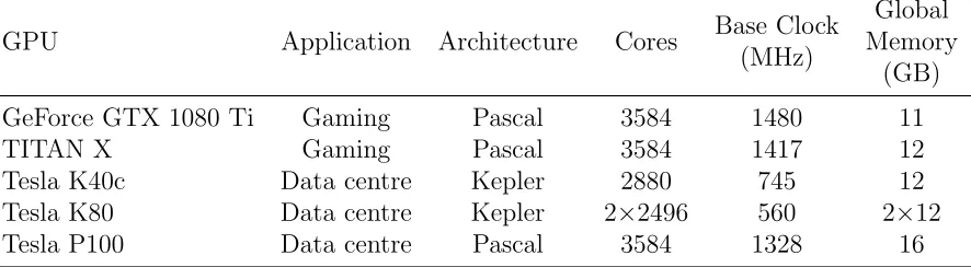
GeForce GTX 1080 Ti Gaming Pascal 3584 1480 11
TITAN X Gaming Pascal 3584 1417 12
Tesla K40c Data centre Kepler 2880 745 12
Tesla K80 Data centre Kepler 2×2496 560 2×12
Tesla P100 Data centre Pascal 3584 1328 16
Table 1: NVIDIA GPU general specifications
3. Performance analysis
The host machine used to carry out performance comparisons between the CPU and GPU-accelerated solvers was a SuperMicro SYS-7048GR-TR with 2 x Intel Xeon E5-2640 v4 2.40 GHz processors, 256GB RAM, and CentOS Linux (7.2.1511) operating system. We tested five different NVIDIA GPUs, the specifications of which are given in Table 1. The GPUs feature a mixture of current generation NVIDIA architecture (Pascal) and previous generation (Kepler). The GPUs are also targeted at different applications, with the GeForce GTX 1080 Ti and TITAN X being principally aimed at the computer gaming market, whilst the Tesla K40c, Tesla K80, and Tesla P100 intended to be used in HPC or data centre environments. Before testing our own kernels we ran the BabelStream benchmark [28] to investigate the maximum achievable memory bandwidth for each GPU. Table 2 presents the results of the BabelStream benchmark alongside the theoretical peak memory bandwidth for each GPU. Table 2 shows that reaching between 66% and 75% theoretical peak memory bandwidth is the maximum performance that we can expect to achieve, with the Pascal generation of GPUs capable of achieving closer to their theoretical peak memory bandwidth than the previous Kepler-based GPUs.
GPU
Theoretical Peak Memory Bandwidth
(GB/s)
BabelStream Memory Bandwidth
(GB/s)
Percentage Theoretical
Peak
GeForce GTX 1080 Ti 484 360 74%
TITAN X 480 360 75%
Tesla K40c 288 191 66%
Tesla K80 2×240 160 66%
Tesla P100 732 519 71%
Table 2: NVIDIA GPU memory bandwidth (FP32)
with a waveform of the shape of the first derivative of a Gaussian. The centre frequency of this waveform was 900 MHz. The time histories of the electric and magnetic field components were stored from a single observation point close to the source. Although these initial models are unrepresentative of a typical GPR simulation, they provide a valuable baseline for evaluating the performance of the CPU and GPU-accelerated solvers.
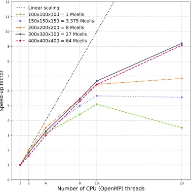
Before evaluating the GPU-accelerated solver an overview of the perfor-mance of the CPU solver is presented in Figures 1 and 2. Figure 1 shows speed-up factors for different sizes of test model using different numbers of OpenMP threads – from a single thread up to the total number of physical CPU cores available on the host machine (2×10 = 20 threads), i.e. strong scaling. For smaller simulations (<≈3 million cells or 1443 model), on this host machine, using more than 10 threads has no impact, or is even detri-mental, to performance. This is likely because the computational overhead of creating and destroying the additional threads is greater than the time saved by having more threads doing work. The speed-up trend converges as the number of cells increase, and is almost identical for the 3003 and 4003 mod-els. At this point the work done by each thread has exceeded the overhead of creating and destroying the thread. The overall speed-up trend decreases beyond 4-8 threads, and falls to around 50% with 20 threads. We would only expect to see ideal speed-up if our algorithm was compute (or cache) bound. Our algorithm is bound by memory bandwidth which is a shared resource across threads. Although adding more threads allows a higher per-centage of this to be used, it is not a linear correlation due to the nature of the hardware. Also depending on where the data is allocated on memory
1 2 4 8 10 20
Number of CPU (OpenMP) threads
0 1 2 3 4 5 6 7 8 9 10 11 12
Speed-up factor
Linear scaling
100x100x100 = 1 Mcells
150x150x150 = 3.375 Mcells
200x200x200 = 8 Mcells
300x300x300 = 27 Mcells
400x400x400 = 64 Mcells
Figure 1: Strong scaling CPU solver performance (speed-up compared to a single thread). Different cubic sizes of model domain compared with different numbers of OpenMP threads. CPU: 2 x Intel Xeon E5-2640 v4 2.40 GHz
1 2 4 8
Number of CPU (OpenMP) threads
150 160 170 180 190 200 210 220 230 240 250
Time [s]
Ideal scaling
100x200x200 = 4 Mcells
200x200x200 = 8 Mcells
200x200x400 = 16 Mcells
200x400x400 = 32 Mcells
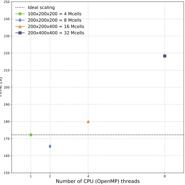
Figure 2: Weak scaling CPU solver performance (execution time compared to a single thread). Size of model domain is increased in proportion to number of OpenMP threads. CPU: 2 x Intel Xeon E5-2640 v4 2.40 GHz
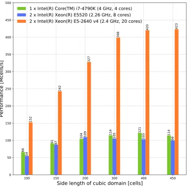
A more useful benchmark of performance is to measure the throughput of the solver, typically given by (2).
P = N X·N Y ·N Z ·N T
T ·1×10⁶ , (2)
whereP is the throughput in millions of cells per second; N X,N Y, andN Z are the number of cells in domain in the x, y, and z directions; N T is the
100 150 200 300 400 450
Side length of cubic domain [cells]
0 50 100 150 200 250 300 350 400 450 500
Performance [Mcells/s]
66
91 104
114 121 114
54
87
109 105 103
99
152
242
327
398
420 423
1 x Intel(R) Core(TM) i7-4790K (4 GHz, 4 cores)
2 x Intel(R) Xeon(R) E5520 (2.26 GHz, 8 cores)
2 x Intel(R) Xeon(R) E5-2640 v4 (2.4 GHz, 20 cores)
Figure 3: CPU solver performance throughput on different CPUs
number of time-steps in the simulation; andT is the runtime of the simulation in seconds. Figure 3 shows comparisons of performance throughput for the CPU solver on different CPUs: 1× Core i7-4790K CPU (4 GHz, 4 cores), 2× Xeon E5520 (2.26 GHz, 8 cores), and 2× Xeon E5-2640 v4 (2.4 GHz, 20 cores). It is intended to provide an indicative guide to the performance of the CPU solver on three different Intel CPUs from typical desktop and server machines.
GPU
FP32 performance
(TFLOPS)
FP64 performance
(TFLOPS)
GeForce GTX 1080 Ti 11.3 0.35
TITAN X 11 0.34
Tesla K40c 4.29 1.43
Tesla K80 8.74 2.91
Tesla P100 10.6 5.3
Table 3: NVIDIA GPU floating point (FP) performance
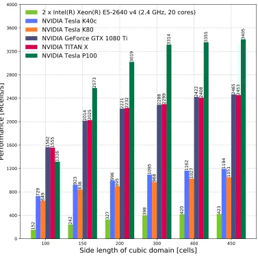
CPU solver (using 2× Xeon E5-2640 v4 (2.4 GHz, 20 cores)) and the GPU-accelerated solver on the five different NVIDIA GPU cards. The Kepler-based Tesla K40c and Tesla K80 exhibit similar performance to one another, and the Pascal-based TITAN X and GeForce GTX 1080 Ti also have similar performance to one another in all the tests. This is expected given these cards have similar memory bandwidth. The TITAN X and GeForce GTX 1080 Ti performance is approximately twice the throughput of the Kepler cards. The Tesla P100 has the highest memory bandwidth, and also has the highest performance throughput. The performance throughput for all the GPUs begins to plateau for models sizes of 3003 and larger, which is because the arrays that the kernels are operating on become large enough to saturate the memory bandwidth.
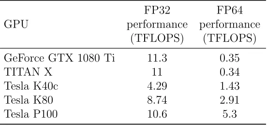
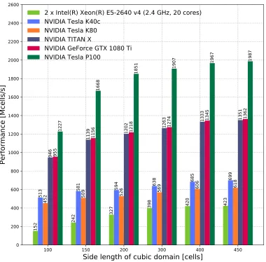
We investigated both single and double precision performance, as for many GPR simulations single precision output provides sufficient accuracy. Table 3 shows that the Tesla-series cards have peak double precision perfor-mance that is half of their peak single precision perforperfor-mance. The TITAN X and GeForce GTX 1080 Ti are designed for single precision performance, so their double precision performance is worse than half of the single preci-sion performance. However, as previously explained the performance of our GPU kernels is governed by memory bandwidth rather than floating point performance. Figures 4 and 5 show that the performance of the Tesla-series GPUs as well as the TITAN X and GeForce GTX 1080 Ti GPUs halves when comparing double to single precision. This reduction in performance happens because twice the amount of data is being loaded/stored for the double precision results, so the time doubles because the memory bandwidth is fixed.
100 150 200 300 400 450
Side length of cubic domain [cells]
0 400 800 1200 1600 2000 2400 2800 3200 3600 4000
Performance [Mcells/s]
152 242
327 398 420 423
729
923 996
1095 1162 1194
649
838 895 968
1027 1051
1562
2014
2221 2288
2422 2465
1555
2025
2232 2299
2408 2453
1316
2573
3019
3314 3355 3405
2 x Intel(R) Xeon(R) E5-2640 v4 (2.4 GHz, 20 cores)
NVIDIA Tesla K40c
NVIDIA Tesla K80
NVIDIA GeForce GTX 1080 Ti
NVIDIA TITAN X
NVIDIA Tesla P100
Figure 4: CPU solver and GPU-accelerated solver performance throughput (FP32)
100 150 200 300 400 450
Side length of cubic domain [cells]
0 200 400 600 800 1000 1200 1400 1600 1800 2000 2200 2400 2600
Performance [Mcells/s]
152 242
327 398
420 423
513 581 594
638 685 699
452 509 526
569 606 618
946
1139 1202
1263 1333 1351
955
1156 1218
1274 1345 1362
1227
1668
1851 1907
1967 1987
2 x Intel(R) Xeon(R) E5-2640 v4 (2.4 GHz, 20 cores)
NVIDIA Tesla K40c
NVIDIA Tesla K80
NVIDIA TITAN X
NVIDIA GeForce GTX 1080 Ti
NVIDIA Tesla P100
Figure 5: CPU solver and GPU-accelerated solver performance throughput (FP64)
4. GPR Example Simulations
Following the initial performance assessment of the GPU-accelerated solver with simple models, we carried out further testing with more realistic, rep-resentative models for GPR. Both of the presented example simulations use some of the advanced features of gprMax such as: modelling dispersive media (for which GPU kernels have been written) using multi-pole Debye expres-sions; soil modelling using a semi-empirical formulation for dielectric proper-ties, and fractals for geometric characteristics; rough surface generation; and
CPU/GPU Name A-scan runtime [s]
Performance [Mcells/s]
2 x Intel(R) Xeon(R) E5-2640 v4 922 127
GeForce GTX 1080 Ti 161 726
TITAN X 162 721
Tesla K40c 374 312
Tesla K80 389 300
Tesla P100 129 906
Table 4: Buried utilities model: A-scan runtimes and performance throughput on different NVIDIA GPUs
the ability to embed complex transducers.
4.1. Buried utilities model
Figure 6: FDTD mesh of a typical GPR environment for detecting and locating buried pipes and cables
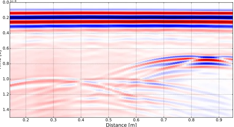
Figure 7 shows the results of the complete simulation, which is a B-scan composed of 91 A-scans with an inline spacing of 10 mm4. The interpretation of the B-scan is not the subject of this paper, but typical hyperbolic responses from the cylindrical targets can be observed, including responses from the top and bottom surface of the air-filled HDPE pipe. The B-scan was simulated utilising the MPI task farm functionality of gprMax, which allows models (A-scans in this case) to be task farmed as MPI tasks using either the CPU or GPU-accelerated solver. For the B-scan model the host machine was fitted with 2× GeForce GTX 1080 Ti GPUs and 2× TITAN X GPUs, and the MPI task farm functionality was used to run 4 A-scans at once in parallel, i.e. one on each of the GPUs. The B-scan simulation (91 A-scans) required
4The only processing of the B-scan data was to apply a quadratic gain function to enhance the target responses in the lossy soil.
0.2 0.3 0.4 0.5 0.6 0.7 0.8 0.9
Distance [m]
0.0
0.2
0.4
0.6
0.8
1.0
1.2
1.4
Time [s]
1e 8
Figure 7: B-scan data from a typical GPR environment containing buried pipes and cables
at total of 1 hour 17 minutes and 56 seconds to run on the GPUs. This would have required 23 hours and 20 minutes to run on host with the parallelised (OpenMP) CPU solver.
4.2. Anti-personnel landmine model
Parameter Value
Domain size (x,y,z) 1.5×1.2×0.328 m Spatial resolution (x,y,z) 0.002×0.002×0.002 m Temporal resolution 3.852×10⁻¹²s
Time window 8×10⁻⁹s
A-scan sampling interval 0.010 m
A-scans per B-scan 121
B-scan spacing 0.025 m
Number of B-scans (x,y) 37×37
Surface roughness (about mean height) ±0.010 m
Table 5: Key parameters for buried landmine model
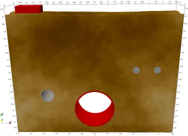
landmine models – 2× PMN and 1× PMA-1; a heterogeneous soil with a rough surface; a GPR antenna model; a false metal target; and several rocks.
The simulation required a total of 121×37×2 = 8954 models (A-scans) to image the entire space. An example of one of the B-scans from the simulation is given in Figure 9. We carried out the simulations on Tesla P100 GPUs on NVIDIA DGX-1 systems that were part of the Joint Academic Data science Endeavour (JADE) computing facility funded by the Engineering and Physical Sciences Research Council (EPSRC). We were able to use 11 nodes of JADE, where each node contained 8 Tesla P100 GPUs. Each model required 96 s runtime, and therefore the total time to complete the simulation (8954 models) was 2 hours and 44 minutes. This level of performance for such large-scale, realistic GPR simulations would simply not be attainable without the GPU-accelerated solver. It is a significant advancement for areas of GPR research like full-waveform inversion and machine learning, where many thousands of forward models are required.
5. Conclusion
We have developed a GPU-accelerated FDTD solver using NVIDIA’s CUDA framework, and integrated it into open source EM simulation soft-ware for modelling GPR. We benchmarked our GPU solver on a range of Kepler- and Pascal-based NVIDIA GPUs, as well as compared performance to the parallelised (OpenMP) CPU solver on a range of desktop and server
Figure 8: FDTD mesh of a complex GPR environment for detecting and locat-ing buried anti-personnel landmines. The model contains: buried anti-personnel landmines – 2×PMN (blue) and 1×PMA-1 (green); a heterogeneous soil with a rough surface (not shown); a GPR antenna model (red); a false metal target (light grey cylinder); and several rocks (dark grey).
specification Intel CPUs. Simple models that contained non-dispersive ma-terials and a Hertzian dipole source achieved performance throughputs of up to 1194 Mcells/s and 3405 Mcells/s on Kepler and Pascal architectures, respectively. This is up to 30 times faster than the OpenMP CPU solver can achieve on a commonly-used desktop CPU (Intel Core i7-4790K). We found the performance of our GPU kernels was largely dependant on the memory bandwidth of the GPU, with the Tesla P100, which had the largest peak theoretical memory bandwidth of the cards we tested (732 GB/s), exhibiting the best performance.
Figure 9: B-scan data from a GPR environment containing buried anti-personnel landmines, a heterogeneous soil with a rough surface, a GPR antenna model, a false metal target, and rocks.
GTX 1080 Ti, to be especially notable, potentially allowing many individ-uals to benefit from this work using commodity workstations. Additionally the equivalent Telsa series P100 GPU (targeted towards data-centre usage) demonstrated significant overall performance advantages due to its use of high bandwidth memory. These benefits can be further enhanced when com-bined with our MPI task farm that enables several GPUs to be used in parallel. We expect performance benefits of our GPU solver to rapidly ad-vance GPR research in areas such as full-waveform inversion and machine learning, where typically many thousands of forward simulations require to be executed.
Acknowledgment
The authors would like to acknowledge Google Fiber (USA) for providing financial support for this work.
The authors would also like to acknowledge the use of the Joint Academic Data science Endeavour (JADE) Tier 2 computing facility funded by the Engineering and Physical Sciences Research Council (EPSRC).
References
References
[1] J. Nickolls, I. Buck, M. Garland, K. Skadron, Scalable parallel program-ming with cuda, Queue 6 (2) (2008) 40–53.
[2] K. S. Yee, Numerical solution of initial boundary value problems involv-ing maxwells equations in isotropic media, Antennas and Propagation, IEEE Transactions on 14 (3) (1966) 302–307.
[3] Acceleware. Axfdtd solver [online, cited 2017-05-09].
[4] Computer Simulation Technology. Cst microwave studio [online, cited 2017-05-09].
[5] SPEAG. Semcad x [online, cited 2017-05-09].
[6] P. Wahl, D.-S. Ly-Gagnon, C. Debaes, D. A. Miller, H. Thienpont, B-calm: An open-source gpu-based 3d-fdtd with multi-pole dispersion for plasmonics, in: Numerical Simulation of Optoelectronic Devices (NU-SOD), 2011 11th International Conference on, IEEE, 2011, pp. 11–12.
[7] P. Klapetek. Gsvit [online, cited 2017-05-09].
[8] Korea University ElectroMagnetic wave Propagator. Kemp [online, cited 2017-05-09].
[9] S. Busch, J. van der Kruk, J. Bikowski, H. Vereecken, Quantitative conductivity and permittivity estimation using full-waveform inversion of on-ground gpr data, Geophysics 77 (6) (2012) H79–H91.
[11] I. Giannakis, A. Giannopoulos, C. Warren, A machine learning approach for simulating ground penetrating radar, in: 2018 17th International Conference on Ground Penetrating Radar (GPR), 2018, pp. 1–4. doi: 10.1109/ICGPR.2018.8441558.
[12] N. J. Cassidy, T. M. Millington, The application of finite-difference time-domain modelling for the assessment of gpr in magnetically lossy mate-rials, Journal of Applied Geophysics 67 (4) (2009) 296–308.
[13] P. Shangguan, I. L. Al-Qadi, Calibration of fdtd simulation of gpr signal for asphalt pavement compaction monitoring, Geoscience and Remote Sensing, IEEE Transactions on 53 (3) (2015) 1538–1548.
[14] E. Slob, M. Sato, G. Olhoeft, Surface and borehole ground-penetrating-radar developments, Geophysics 75 (5) (2010) 75A103–75A120.
[15] F. Soldovieri, J. Hugenschmidt, R. Persico, G. Leone, A linear inverse scattering algorithm for realistic GPR applications, Near Surface Geo-physics 5 (1) (2007) 29–42.
[16] M. Solla, R. Asorey-Cacheda, X. N´u˜nez-Nieto, B. Conde-Carnero, Eval-uation of historical bridges through recreation of gpr models with the fdtd algorithm, NDT & E International 77 (2016) 19–27.
[17] A. P. Tran, F. Andre, S. Lambot, Validation of near-field ground-penetrating radar modeling using full-wave inversion for soil moisture es-timation, Geoscience and Remote Sensing, IEEE Transactions on 52 (9) (2014) 5483–5497.
[18] C. Warren, A. Giannopoulos, I. Giannakis, gprmax: Open source soft-ware to simulate electromagnetic wave propagation for ground penetrat-ing radar, Computer Physics Communications 209 (2016) 163–170.
[19] I. Giannakis, A. Giannopoulos, A novel piecewise linear recursive con-volution approach for dispersive media using the finite-difference time-domain method, IEEE Transactions on Antennas and Propagation 62 (5) (2014) 2669–2678.
[20] I. Giannakis, A. Giannopoulos, C. Warren, A realistic fdtd numerical modeling framework of ground penetrating radar for landmine detection,
IEEE Journal of Selected Topics in Applied Earth Observations and Remote Sensing 9 (1) (2016) 37–51.
[21] A. Giannopoulos, Unsplit implementation of higher order pmls, IEEE Transactions on Antennas and Propagation 60 (3) (2012) 1479–1485.
[22] C. Warren, A. Giannopoulos, Creating finite-difference time-domain models of commercial ground-penetrating radar antennas using taguchi’s optimization method, Geophysics 76 (2) (2011) G37–G47.
[23] A. Taflove, S. C. Hagness, Computational electrodynamics, Artech house, 2005.
[24] S. Williams, A. Waterman, D. Patterson, Roofline: An insightful visual performance model for multicore architectures, Commun. ACM 52 (4) (2009) 65–76. doi:10.1145/1498765.1498785.
URL http://doi.acm.org/10.1145/1498765.1498785
[25] M. Livesey, J. F. Stack, F. Costen, T. Nanri, N. Nakashima, S. Fujino, Development of a cuda implementation of the 3d fdtd method, IEEE Antennas and Propagation Magazine 54 (5) (2012) 186–195.
[26] T. Nagaoka, S. Watanabe, A gpu-based calculation using the three-dimensional fdtd method for electromagnetic field analysis, in: Engi-neering in Medicine and Biology Society (EMBC), 2010 Annual Inter-national Conference of the IEEE, IEEE, 2010, pp. 327–330.
[27] J. Stack, Accelerating the finite difference time domain (fdtd) method with cuda, in: Appl. Comput. Electromagn. Soc. Conf, 2011.
[28] T. Deakin, J. Price, M. Martineau, S. McIntosh-Smith, Gpu-stream v2.0: Benchmarking the achievable memory bandwidth of many-core processors across diverse parallel programming models, in: First Inter-national Workshop on Performance Portable Programming Models for Accelerators (P3MA), 2016.