A New Analytical Procedure to solve Two phase Flow
in Tubes
Terry Moschandreou1,2,∗,†ID
1 Fanshawe College; [email protected]
2 Western University; [email protected]
* Correspondence: [email protected]; Tel.: 1-519-452-4430 † 1001 Fanshawe College Blvd,London Ontario, Canada
Abstract:A new formulation for a proposed solution to the 3D Navier-Stokes Equations in cylindrical 1
co-ordinates coupled to the continuity and level set convection equation is presented in terms of an 2
additive solution of the three principle directions in the radial, azimuthal andzdirections of flow and 3
a connection between the level set function and composite velocity vector for the additive solution is 4
shown. For the case of a vertical tube configuration with small inclination angle, results are obtained 5
for the level set function defining the interface in both the radial and azimuthal directions. It is found 6
that the curvature dependent part of the problem alone induces sinusoidal azimuthal interfacial 7
waves wheras when the curvature is small oscillating radial interfacial waves occur. The implications 8
of two extremes indicate the importance of looking at the full equations including curvature. 9
Keywords:Fluid dynamics, Two phase flow, Level set function, Cylindrical coordinates, Continuity 10
equation 11
1. Introduction 12
The level set method, has been used originally as a numerical technique for tracking interfaces 13
and shapes [3],[4] and has been increasingly applied to various areas of engineering and applied 14
mathematics. In the level set method, contours or surfaces are represented as the zero level set of a 15
higher dimensional function called a level set function. This can be the distance from the particular 16
phase of material to the interface. For example in fracture mechanics level set methods have been 17
used to track the shape around a crack in two and three dimensions that is propagating with a sharp 18
kink [7].Also various applications in image segmentation have been used with corresponding active 19
curve evolution algorithms [2],[6].Reachability analysis is frequently used to study the safety of control 20
systems. Using exact reachability operators for nonlinear hybrid systems is presented in [9]. An 21
algorithm for determining reachable sets and synthesizing control laws is implemented using level 22
set methods in [9]. Various models used to compute the interaction of 3D incompressible fluids with 23
elastic membranes or bodies, rely on the use of level set functions [10], to capture the fluid-solid 24
interfaces and to measure elastic stresses that have been used. In [10] the computation of equilibrium 25
shapes of biological vesicles is presented and numerical simulations of spontaneous cardiomoyocyte 26
contractions is presented. A conservative method of level set type for moving interfaces in divergence 27
free velocity fields is presented in [5], [8]. The method in [8] was coupled to a Navier-Stokes solver 28
for incompressible two phase flow with surface tension. Wave phenomena is known to exist at the 29
interface of two phase immiscible flows [11]. In the present paper we present a level set method for 30
moving interfaces for such velocity fields which are coupled to Navier-Stokes equations for two phase 31
flows in tubes.The novelty of the present work is to reveal an analytical approach in solving the 3D 32
cylindrical Navier-Stokes equations where the three principle directions of flow, in radial, azimuthal 33
and longitudinal directions are summed to form a new composite vector velocity expression. In this 34
light we propose to solve a curvature only formulation of the governing equation for the level set 35
function and one in which the curvature is removed from the governing equation. 36
1.1. Level Sets in Cylindrical Co-ordinates 37
Letφbe a level set function.[1],[3]. The gradient of the level set function in cylindrical co-ordinates
38
is defined as: 39
40
∇φ=
∂φ ∂r,
1 r
∂φ ∂θ,
∂φ ∂z
(1)
The mean curvature,κ, of the interface defined by the zero isocontour of the level set functionφ, [1],[3],
is the divergence of the normal to the interface given by
~n= ∇φ
|∇φ| (2)
Thus it can be expressed as:
κ=−∇ ·~n (3)
The mean curvatureκof a dynamic surfaceφ(r,θ,z,t) =ψ(r,θ,t) +zin cylindrical co-ordinates is,
41
κ= 1
S "
∂
∂rφ(r,θ,z,t)
r2
∂
∂rφ(r,θ,z,t)
2 +1
! +
2
∂
∂θφ(r,θ,z,t) ∂
∂θφ(r,θ,z,t)−r ∂2
∂θ∂rφ(r,θ,z,t)
! +
r
∂
∂θφ(r,θ,z,t)
2 +r2
!
∂2
∂r2φ(r,θ,z,t) +
r
∂2
∂θ2φ(r,θ,z,t)
∂
∂rφ(r,θ,z,t)
2 +1
! #
(4)
where
S= 2r2
∂
∂rφ(r,θ,z,t)
2 +1
! +2
∂
∂θφ(r,θ,z,t)
2!3/2
(5)
The geometric trace of a dynamic closed surface that bounds an open set can be represented implicitly as
S={(r,θ,z,t)|φ(r,θ,z,t) =0} (6)
and for two phase flow has two separate regions whereφ>0 andφ<0 respectively.[1] The surface
evolution is determined by:
φt=u· ∇φ (7)
The Navier–Stokes Equations are:
∂u
∂t + (u· ∇)u=−
1
ρ∇p+µ∇
2u+ 1
where for cylindrical(r,θ,z)coordinate system, Laplace operator has the form
∇2=
∂2 ∂r2 +
1 r
∂ ∂r
| {z }
1
r∂∂r(r∂∂r) +1
r2
∂2 ∂θ2 +
∂2 ∂z2
and the gradient is is given by Eq.(1) 42
1.2. A new composite velocity formulation 43
The 3D cylindrical incompressible unsteady Navier-Stokes equations coupled to interface convection equation are written in expanded form, for each component, ur,uθanduz, where the
remaining non linear terms appearing in full N.S equations are suppressed for the time being:
urt+ur∂ur
∂r +
uθ
r
∂ur ∂θ +uz
∂ur ∂z −
µ ρ
−ur
r2 +
∂2ur ∂r2 +
1 r
∂ur ∂r +
1 r2
∂2ur ∂θ2 +
∂2ur ∂z2
+
1
ρ ∂p
∂r −Fgr−
1
ρσκ ∂φ
∂r =0 (8)
uθt+ur∂uθ
∂r +
uθ
r
∂uθ ∂θ +uz
∂uθ ∂z −
µ ρ
−uθ
r2 +
∂2uθ ∂r2 +
1 r
∂uθ ∂r +
1 r2
∂2uθ ∂θ2 +
∂2uθ ∂z2
+
1
ρ ∂p
∂θ −Fgθ−
1
ρσκ
1 r
∂φ
∂θ =0 (9)
uzt+ur∂uz
∂r +
uθ
r
∂uz ∂θ +uz
∂uz ∂z −
µ ρ
∂2uz ∂r2 +
1 r
∂uz ∂r +
1 r2
∂2uz ∂θ2 +
∂2uz ∂z2
+
1
ρ ∂p
∂z −Fgz−
1
ρσκ ∂φ
∂z =0 (10)
44
and whereρis density,µis dynamic viscosity ,Fgr,Fgθ,Fgzare body forces on fluid andσis surface
45
interfacial tension. 46
47
Multiplying Eqs(8-10) by unit vectors ~er, ~eθ and ~k respectively and adding Equations (8-10)
48
gives the following equation, for~L=ur~er+uθ~eθ+uz~k,
49
~Lt+ur∂~L
∂r +
uθ
r
∂~L ∂θ +uz
∂~L ∂z −
µ ρ −
~L
r2+
∂2~L ∂r2 +
1 r
∂~L ∂r +
1 r2
∂2~L ∂θ2 +
∂2~L ∂z2
! + 1
ρPT−FT−
1
ρσκ
~L=0 (11)
co-ordinates:
φt+ur
∂φ ∂r +
uθ
r
∂φ ∂θ +uz
∂φ
∂z =0 (12)
The continuity equation in cylindrical co-ordinates is
∂ρ ∂t +ur
∂ρ ∂r +
uθ
r
∂ρ ∂θ +uz
∂ρ ∂z =−ρ
∂ur ∂r +
1 r
∂uθ ∂θ +
∂uz ∂z
(13)
Multiply Eq(11) by ρ µφ:
ρ µ[φ
~Lt+φur∂~L
∂r +φ
uθ
r
∂~L ∂θ +φuz
∂~L ∂z− µ
ρφ −
~L
r2+
∂2~L ∂r2 +
1 r
∂~L ∂r +
1 r2
∂2~L ∂θ2 +
∂2~L ∂z2
! +1
ρφPT−φFT−
1
ρσφκ
~L] =0 (14)
Multiply Level set function convection Eq.(12) by ρµ~L:
ρ µ[
~Lφt+~Lur∂φ
∂r +
~Luθ
r
∂φ ∂θ +
~Luz∂φ
∂z] =0 (15)
50
Adding Eqs(14) and (15) gives 51
52
ρ µ[φ
~Lt+~Lφt+φur~Lr+~Lurφr+φuθ
r~Lθ+~L
uθ
r φθ+φuz~Lz+~Luzφz−
µ ρφ −
~L
r2+
∂2~L ∂r2 +
1 r
∂~L ∂r +
1 r2
∂2~L ∂θ2 +
∂2~L ∂z2
! +1
ρφPT−φFT−
1
ρσφκ
~L] =0 (16)
By product rule we rewrite the previous equation as:
ρ µ[(φ
~L)t+ (φur~L)r+1
r(φuθ~L)θ+ (φuz~L)z]−
φ −
~L
r2 +
∂2~L ∂r2 +
1 r
∂~L ∂r +
1 r2
∂2~L ∂θ2 +
∂2~L ∂z2
! + 1
µφPT− ρ µφFT−
1
µσφκ
~L=0 (17)
and sinceφis usually taken to be a distance function from the interface we can consider the following
expression in terms ofφ:
~L(r,θ,z,t) = 1
φ µ ρ
~L (18)
where µρ has SI units of ms2 and ~L = φr~er + 1rφθ~ezθ+φz~z is by definition in Navier Stokes
equation(Eqs(8-10)) of dimensionm1 andφis dimensionless.
From Level set Eq(7),
~L~L·~L=−~L(φt) (19)
53
From the first line of Eq.(17) using Eq(18) we have a derivative term int, first we write: 54
55
56
µ ρ
~L= (µ1+ (µ2−µ1)φ(r,θ,z,t))~L(r,θ,z,t)
ρ1+ (ρ2−ρ1)φ(r,θ,z,t) (20)
where
ρ=ρ1+ (ρ2−ρ1)φ, µ=µ1+ (µ2−µ1)φ
and
µ ρ
~L
t
=−
∂
∂tφ(r,θ,z,t)
~L(r,θ,z,t) ((ρ2−ρ1)µ1−(µ2−µ1)ρ1)
(ρ1+ (ρ2−ρ1)φ(r,θ,z,t))2
+
(µ1+ (µ2−µ1)φ(r,θ,z,t)) ∂∂t~L(r,θ,z,t)
ρ1+ (ρ2−ρ1)φ(r,θ,z,t) (21)
and for derivative terms inr,θ,z, from the first line of Eq.(17) we have,
N1 D1+
N2 D2 +
N3
D2, (22)
N1=~L(r,θ,z,t) ((ρ2−ρ1)µ1−(µ2−µ1)ρ1)×
ur
∂
∂rφ(r,θ,z,t)
r+uθ ∂
∂θφ(r,θ,z,t) +uz
∂
∂zφ(r,θ,z,t)
r
(23)
N2= (µ1+ (µ2−µ1)φ(r,θ,z,t))×
ur ∂
∂r
~L(r,θ,z,t) +uθ∂θ∂~L(r,θ,z,t)
r +uz
∂ ∂z
~L(r,θ,z,t)
!
(25)
N3= (µ1+ (µ2−µ1)φ(r,θ,z,t))×
~L ∂
∂rur(r,θ,z,t) +
~L ∂
∂θuθ(r,θ,z,t)
r +~L
∂
∂zuz(r,θ,z,t)
!
(26)
D2=ρ1+ (ρ2−ρ1)φ(r,θ,z,t) (27)
57
58
1.3. Special Case Solution 59
In this section it is assumed that the tube is in a vertical configuration with a small inclination angle and
(ρ2−ρ1)µ1−(µ2−µ1)ρ1=0 (28) Equation(26) can be rewritten using the time dependent continuity equation Eq(13),
60
61
−ρ× ~L ∂
∂rur(r,θ,z,t) +
~L ∂
∂θuθ(r,θ,z,t)
r +~L
∂
∂zuz(r,θ,z,t)
! =~L
∂ρ ∂t +
~L· ∇ρ
(29)
∇ρ= 1
γ∇φ (30)
Use of Eq.(17), Eqs.(22-30) gives a non-linear PDE
ρ µ(φ
~L)t+ ρ
µ
~L· ∇~L+1
ρ
~L∂ρ
∂t +1 ρ ρ γµ
~L~L· ∇φ−
φ −
~L
r2 +
∂2~L ∂r2 +
1 r
∂~L ∂r +
1 r2
∂2~L ∂θ2 +
∂2~L ∂z2
! + 1
µφ
~
PT−
ρ µφ
~
FT− 1
µσφκ
~L=0 (31)
φ~Lt−φ ∂
2~L
∂r2
+1 r
∂~L ∂r +
1 r2
∂2~L ∂θ2
+∂ 2~L
∂z2
! + 1
µφ
~
PT−
ρ µφ
~
FT−
1
µσφκ
~L+
~Ψ(r,ur,uθ,∂ur
∂θ , ∂uθ
∂θ ) =0 (32)
A solution of the algebraic equation (28) gives as one special solutionµ1=0 andρ1=0, withµ2and
product in Eq(19), withΨdefined as the numerator ofκappearing in Eq.(4), Eq.(31) reduces to
Fz+
∂
∂t~L(r,θ,t)
φ(r,θ,t) −
~L(r,θ,t)
φ(r,θ,t)
Ψ
−∂∂tφ(r,θ,t)
φ(r,θ,t)
3/2+
~L(r,θ,t)
r2φ(r,θ,t)−
∂2 ∂r2
~L(r,θ,t)
φ(r,θ,t) +2×
∂
∂r~L(r,θ,t)
∂
∂rφ(r,θ,t)
(φ(r,θ,t))2
−2
~L(r,θ,t)∂
∂rφ(r,θ,t)
2
(φ(r,θ,t))3
+
~L(r,θ,t) ∂2
∂r2φ(r,θ,t)
(φ(r,θ,t))2
−
1 r
∂
∂r~L(r,θ,t)
φ(r,θ,t) −
~L(r,θ,t) ∂
∂rφ(r,θ,t)
(φ(r,θ,t))2
! − 1 r2 ∂2 ∂θ2
~L(r,θ,t)
φ(r,θ,t) −2
∂
∂θ~L(r,θ,t)
∂
∂θφ(r,θ,t)
(φ(r,θ,t))2
+2
~L(r,θ,t)∂
∂θφ(r,θ,t)
2
(φ(r,θ,t))3
−~L(r,θ,t) ∂2
∂θ2φ(r,θ,t)
(φ(r,θ,t))2
+
~L(r,θ,t)
(φ(r,θ,t))2 ∂ ∂r
~L(r,θ,t) + ∂θ∂~L(r,θ,t)
r !
=0 (33)
,Fzis force of gravity in inclined tube. 62
1.3.1. Curvature Term Omitted 63
In this first part we solve Eq.(33) with the curvature partΨ ignored. This is because we can subsititute~L = ∇φand setφ = eαtF(r,θ)for α < 0 andtsufficiently large to cancel terms with αand t. With curvature term dropped it can be proven that F(r,θ)is multiplicatively separable,
F(r,θ) = f(r)g(θ)and we obtain the following,
d3
dr3f(r) =−
d drf(r)
2 c1 f(r)r + Fz r2(f(r))3+
4ddr22f(r)
r2d
drf(r)
f(r)−2 ddrf(r)3r2−(f(r))2 d2
dr2f(r)
r+ (f(r))2 ddrf(r) (f(r))2r2
(34)
64
65
d
dθg(θ) =−g(θ)c1−g(θ) (35)
Setting f(r) = exp(G(r))andG(r) = ln(H(r))in Eq.(34) and factoring exponential terms out we obtain,
2
d drH(r)
3
(H(r))3 −4
d2 dr2H(r)
d drH(r)
(H(r))2 + d3 dr3H(r)
H(r) + d2 dr2H(r)
rH(r) +
d drH(r)
2 c1 r(H(r))2 − d
drH(r)
r2H(r) −Fz=0 (36)
H(r) =Y(r),
d2
dr2Y(r)−
4 (Ω(r))2r2−2 ddrΩ(r)r2−Ω(r)rddrY(r)
Ω(r)r2 −
−2 (Ω(r))3r2+Fzr2−(Ω(r))2c1r+4Ω(r)ddrΩ(r)r2−d2 dr2Ω(r)
r2−d drΩ(r)
r+Ω(r)Y(r)
Ω(r)r2 =0
(37)
If Eq.(37) has closed form solutions then the pseudo-exact form, [13], of Eq.(37) has solutions which are given by,
2 (Ω(r))3r−F zr+ (Ω(r))2c1+4ddrΩ(r)rΩ(r)
r =1 (38)
Equation(38) can be rewritten as an Abel equation of the second kind which can be transformed into an Abel equation of the first kind
d
dry(r) =−1/2+ (B/4+1/4) (y(r)) 3−
1/4y(r)
r (39)
where force of gravity inzdirection is,
B=Fz (40)
and
Ω(r) = 1
y(r) (41)
Equation (39) solved due to [12] can be written as follows,
d
dru(r) =−
22/3(u(r))3
r +
22/3u(r)β
r +1/2
22/3u(r) r2 −
22/3
r −
u(r) r2
3
q
−(B+1)−1 (42)
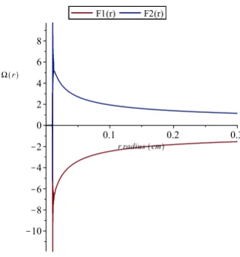
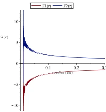
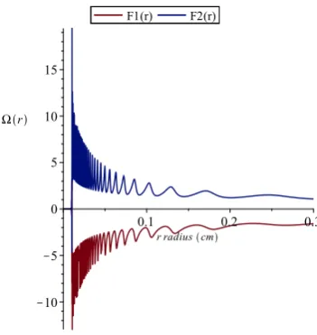
66
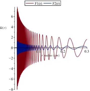
where the transformationy(r) =−B+21u(r), for chosenβis used. IfB >−1 then we have complex
67
equation and can be written as a real and imaginary part,F1(r) =Re(u(r))andF2(r) =Im(u(r)). 68
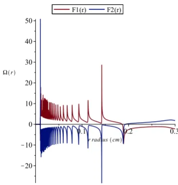
Defining A = −i3 q
−(Fz+1)−1, see Figs (1-5) for Re(A) ranging from low to high values 69
corresponding to various heights in the inclined tube. Here two phases flow upward in tube with 70
greater mass associated with higher positions of fluid column in tube. 71
72
1.3.2. Consideration of Curvature Alone 73
Secondly we solve the curvature pde given in Eq. (4) alone appearing asΨin Eq.(33). This is due to large time evolution of Eq(33). For small inclination angle of tube Eq.(4) reduces to,
−
∂
∂rφ(r,θ,t)
r2∂
∂tφ(r,θ,t)
φ(r,θ,t) +
∂2
∂r2φ(r,θ,t)
r3−r
∂2
∂θ2φ(r,θ,t)
∂
∂tφ(r,θ,t)
which is separable into,
d2
dr2f1(r) =
f1(r)c3c2
r2 +
d drf1(r)
c3
r (44)
d2
dθ2f2(θ) =c2f2(θ) (45)
d
dtf3(t) =c3f3(t) (46)
For constant c2 negative there is a sinusoidal component of the azimuthal part of 74
φ(r,θ,t) = f1(r)f2(θ)f3(t).
75
76
2. Discussion 77
It is worthy to note that the interfacial oscillations occurring as extremes of two problems one 78
for no curvature and the other for curvature alone presents the daunting problem of solving the full 79
equation of Eq.(33). There is a plethora of results for computational multiphase flow using level set 80
methods. The advantage of the present work lies in that analytical results are possible for the two 81
extreme cases presented. It is conjectured at this point that the combination or full Eq(33) without the 82
small inclination angle, ie approaching a horizontal tube configuration of flow, is non separable due to 83
the inherent complexity of Eq(4) and Eq(33) combined. We can expect that there be a very complex 84
relationship between azimuthal and radial components of~L. Work on the complete problem for this 85
Figure 5.A=34.1375, mass of fluid column in vertical tubem=102 grams.
References 87
88
1. S. Osher, R. Fedkiw, Level Set Methods and Dynamic Implicit Surfaces, Springer-Verlag, Berlin, 2003.
89
2. V. Caselles, F. Catte, T. Coll, and F. Dibos, A geometric model for active contours in image processing, Numer.
90
Math., vol. 66, no. 1, pp. 1-31, Dec. 1993
91
3. S.Osher and J.Sethian, Fronts propagating with curvature-dependent speed: Algorithms based on
92
Hamilton-Jacobi formulations, J. Comp. Phys., vol. 79, no. 1, pp. 12-49, Nov. 1988.
93
4. J. Sethian, Level Set Methods and Fast Marching Methods, Cambridge University Press, Cambridge, 1999.
94
5. M. Sussman, P. Smereka, S. Osher, A level set approach for computing solutions to incompressible two-phase
95
flow, J. Comput. Phys. 114 pp 146-159, 1994.
96
6. Chunming Li, Rui Huang, Zhaohua Ding, J. Chris Gatenby, Dimitris N. Metaxas, A Level Set Method for
97
Image Segmentation in the Presence of Intensity Inhomogeneities With Application to MRI ,IEEE Transactions
98
on Image Processing, 20, no. 7, July 2011.
99
7. Marc Duflot , A study of the representation of cracks with level sets, International Journal for Numerical
100
Methods in Engineering Volume 70, Issue 11, pp 1261-1302, 11 June 2007
101
8. Elin Olsson , Gunilla Kreiss ,A conservative level set method for two phase flow, Journal of Computational
102
Physics 210 (2005) 225-246.
103
9. Ian Mitchell,Claire J. Tomlin,Level Set Methods for Computation in Hybrid Systems, International Workshop
104
on Hybrid Systems: Computation and Control HSCC 2000: Hybrid Systems: Computation and Control pp
105
310-323 |
10. Emmanuel Maitre Thomas Milcenta Georges-Henri Cotteta Annie Raoult Yves Usson , Applications of level
107
set methods in computational biophysics, Mathematical and Computer Modelling, Volume 49, Issues 11-12,
108
June 2009, pp 2161-2169
109
11. A. A. Ayati, P. S. C. Farias, L. F. A. Azevedo, and I. B. de Paula, Characterization of linear interfacial waves in
110
a turbulent gas-liquid pipe flow, Physics of Fluids 29, 062106, pp 1-13, 2017.
111
12. Differentialgleichungen Losungsmethoden und Losungen, E. Kamke, Springer Fachmedien Wiesbaden, 1977.
112
13. M. Saravi, A procedure for solving some second-order linear ordinary differential equations, Applied
113
Mathematics Letters 25, pp 408-411, 2012.
114
Conflicts of Interest:The authors declare no conflict of interest.