Numerical solution of Euler’s rotation equations for a rigid body about a fixed point

Numerical solution of Euler’s rotation equations for a rigid body about a

fixed point

Bo-Hua Sun1

School of Civil Engineering & Institute of Mechanics and Technology Xi’an University of Architecture and Technology, Xi’an 710055, China http://imt.xauat.edu.cn

email: [email protected]

Finding a solution for Euler’s equations is a classic mechanics problem. This study revisits the problem with numerical approaches. For ease of teaching and research, a Maple code comprising 2 lines is written to find a numerical solution for the problem. The study’s results are validated by comparing these with previous studies. Our results confirm the correctness of the principle of maximum moment of inertia of the rotating body, which is verified by thermodynamics. As an essential part of this study, the Maple code is provided.

Keywords: Euler’s equation, rigid body, rotation, Maple

I. INTRODUCTION

The celebrated Euler equations of motion for a rigid body consists of three nonlinear equations, coupled with differential equations, which are known as one of the fa-mous problem in classical mechanics1_{. Solving the Euler} equations has attracted the attention of great scientists for the last 300+ years. Despite great efforts in this re-spect, a complete general analytical solution has yet to be found1–11.

Special cases for which solutions have been found1–7,9–11_{, which include the torque-free rigid} body, and the three (or four) famous integrable cases solved by Euler, Lagrange, and Kovalevskaya3_{. The} Lagrange and Kovalevskaya case that symmetric rigid rotor’s two principal moments of inertia are equal to each other, and double that of the third one, namely I1 =I2 = 2I3, and the Euler case that all the applied

torques are zero (torque-free precession of the rotation axis of the rigid rotor)1,2,4. The desire of searching exact solution on the problem has never been ending, recently, Ershkov14_{, who proposed a new and exact solution for} the Euler equations.

Besides the above few integrable cases, for the most disintegrable case or the heavy asymmetric case, some approximate analytical solutions have been proposed by, for example, Amer and Abady15,16_{studied analytical} so-lutions for the rigid body motion in the presence of gyro-static torques in terms of the axes of rotation. Tsiotras and Longuski12,13, who considered the time evolution of the angular velocity of a spinning rigid body, subject to the torques of the three axes, and proposed an asymp-totic analytic solution.

After more than 300 years of investigations and study-ing the Euler’s equation, it is concluded that no closed solution has been obtained for the general case, while numerical solutions have been used. Although the closed

and approximate analytic solutions have great academ-ic value, they have certain limitations, since all of them involve complicated computations and variable transfor-mations. They may be mathematically correct but the difficulty lies in the computational perspective. In order to overcome this situation, it would be natural thinking to use numerical methods for the general case of the Eu-ler equation. If we use numerical methods, the computer code must be written. However, if one studies the litera-ture carefully, it would not be difficult to find that there is no simple computer program, comprising a few line, which has been reported. Therefore, it is highly demand-ed to have a simple straight-forward numerical program that can be used to compute the problem simply by a click.

This study provides a general Maple code for the nu-merical solution of the Euler equation, namely a simple Maple code comprising merely 2 lines. In Section 3 we compare our results with that of the benchmark from Tsiotras and Longuski’s studies13. In section 4 we in-vestigate the torques as functions of time. In Section 5 we compute an asymmetrical top under the action of a gyrostatic moment, and finally, with discussions and a conclusion. For ease of teaching and research, all Maple codes are provided.

II. EULER’S ROTATION EQUATION AND MAPLE CODE

In mechanics, a rigid body may be defined as a system of particles, as the distances between the particles do not vary. To describe the motion of a rigid body, we use two systems of co-ordinates: a "fixed" (i.e. inertial) system, XY Z, and a moving system,x1=x,x2=y, andx3=z

which is supposed to be rigidly fixed in the body, and to participate in its motion. The origin of the moving system may conveniently be taken to coincide with the

centre of body’s mass7.

A non-symmetric spinning body in space, subject to constant torques and non-zero initial conditions, using Euler’s equations of motion for a rotating rigid body with principal axes at the center of mass, produce the following

I1

dΩ1

dt + (I3−I2)Ω2Ω3=K1,

I2

dΩ2

dt + (I1−I3)Ω1Ω3=K2,

I3

dΩ3

dt + (I2−I1)Ω2Ω1=K3.

(1)

The principal torques acting on the rigid body, namely K1, K2 and K3. The principal angular velocity

compo-nents in the same frame, namely Ω1, Ω2 and Ω3. These

quantities are defined in the moving system x1 = x,

x2=y, andx3=z, namely in the body-fixed frame1–10.

Euler’s equations in 1 are nonlinear differential equa-tions, whose general analytical solutions have not been obtained and might well be impossible to obtain1–10_. Hence, for general cases, or for the asymmetrical top of the Euler equations, numerical solutions are perhaps the only choice.

To obtain the numerical solutions, one can write codes by using various software and languages such as Fortran, C++, Matlab, MATHEMATICA and so on. To obtain simple and short codes, the symbolic software, Maple, was used. Hence, a Maple code was produced for the Euler equations. The code is shown in Table I below.

The code uses the solver x-rkf45 which is implemented based on the fourth-order Runge-Kutta method. The above code was used to compute all case studies and they are shown in the forthcoming sections for given moment of inertiaIk, torquesKk and initial conditionx0,y0 and z0.

III. TSIOTRAS AND LONGUSKI’S BENCHMARK13

In 1996 Tsiotras and Longuski13 _{proposed a novel} ap-proximate solution for the asymmetrical top of Euler’s equations, and presented a numerical example. To vali-date our Maple code, we recomputed the same example and compared it with those of Tsiotras and Longuski13. The data that we used is shown in Table II below.

Using our code for the problem, the results for the different ranges of time are shown in the Fig. 1 below.

The kinetic energyT of the asymmetrical top is shown in Table 2 below.

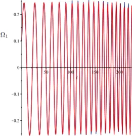
Comparisons of theΩ1 profiles with those of Tsiotras

and Longuski13_{are in shown in Fig.3 below. Our solution} concurs with that of Tsiotras and Longuski13_.

FIG. 1.Ωkprofiles for different time domain obtained by our

Maple code

FIG. 2. 2T = I1(Ω1(t))2 +I2(Ω2(t))2+I3(Ω3(t))2 profiles

obtained by our Maple code

FIG. 3.Ω1profiles’ comparison with Tsiotras and Longuski13,

TABLE I. Maple code for Euler’s equation of a rigid body about a fixed point. The Maple provides simple code comprising 2 line, the first line is list of equations, and the second one is solution

Euler’s equation I1Ω˙1+ (I3−I2)Ω2Ω3=K1, I2Ω˙2+ (I1−I3)Ω1Ω3=K2, I3Ω˙3+ (I2−I1)Ω2Ω1=K3

Equation sys:={I1∗(dif f(Omega1(t),t)) + (I3−I2)∗Omega2(t)∗Omega3(t)−K1 = 0,

I2∗(dif f(Omega2(t),t)) + (I1−I3)∗Omega3(t)∗Omega1(t)−K2 = 0,

I3∗(dif f(Omega3(t),t)) + (I2−I1)∗Omega1(t)∗Omega2(t)−K3 = 0}

Solutiona _{sol:=dsolve({op(sys)}union{Omega1(0) =x0,Omega2(0) =y0,Omega3(0) =z0},}

{Omega1(t),Omega2(t),Omega3(t)},numeric)

Plots odeplot(sol,{[t,Omega1(t)], [t,Omega2(t)], [t,Omega3(t)]},t= 0..t0)

a _{x0,y0 and z0 are the initial condition values}

TABLE II. Data from Tsiotras and Longuski13

Principal moments of inertial [kg.m2_{] I}

1= 3500,I2= 1000,I3= 4200

Applied torque [N.m] K1=−1.2,K2= 1.5,K3= 13.5

Initial conditions x0=0.1, y0=-0.2, z0=0.33

FIG. 4. Ω3profiles’ comparison with Tsiotras and Longuski13,

with the red line showing our results and the blue line showing TL’s results

Comparison of Ω3 profiles with those of Tsiotras and

Longuski13 _{are in shown in Fig.4 below. Our solution} concurs with that of Tsiotras and Longuski13_.

Besides the numerical data is shown in Table IV below, particularly for purpose of future comparative studies.

IV. ELLIPSOID TOP ROTATION

This section demonstrates rotation of ellipsoid top, whose typical shape is shown in Fig. 5 below.

In reality, the torque might depend on the rotation velocity, for instance, in viscous environments. However, there are no results were reported for the torques as func-tions of time. This section demonstrates three examples in this regards, as shown below.

A. Case with one variable torque

If the torque is a function of rotation velocitiy, the code can provide solutions without any difficulty. In this case study, we assume thatK1=−0.1Ω1(t) + 0.05. The other

data is shown in Table IV below.

The results are shown in Fig. 6 below.

FIG. 5. Different angle view of typical asymmetrical ellipsoid top

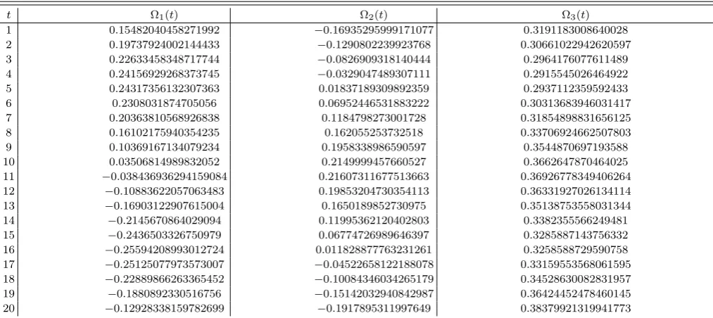
TABLE III. Our numerical results (Note: Ref.13_{did not provide theΩ}

2figure, nor data forΩ1Ω2Ω3.)

t Ω1(t) Ω2(t) Ω3(t)

1 0.15482040458271992 −0.16935295999171077 0.3191183008640028

2 0.19737924002144433 −0.1290802239923768 0.30661022942620597

3 0.22633458348717744 −0.0826909318140444 0.2964176077611489

4 0.24156929268373745 −0.0329047489307111 0.2915545026464922

5 0.24317356132307363 0.01837189309892359 0.2937112359592433

6 0.2308031874705056 0.06952446531883222 0.30313683946031417

7 0.20363810568926838 0.1184798273001728 0.31854898831656125

8 0.16102175940354235 0.162055253732518 0.33706924662507803

9 0.10369167134079234 0.1958338986590597 0.3544870697193588

10 0.03506814989832052 0.2149999457660527 0.3662647870464025

11 −0.038436936294159084 0.21607311677513663 0.36926778349406264

12 −0.10883622057063483 0.19853204730354113 0.36331927026134114

13 −0.16903122907615004 0.1650189852730975 0.35138753558031344

14 −0.2145670864029094 0.11995362120402803 0.3382355566249481

15 −0.2436503326750979 0.06774726989646397 0.3285887143756332

16 −0.25594208993012724 0.011828877763231261 0.3258588729590758

17 −0.25125077973573007 −0.04522658122188078 0.33159553568061595

18 −0.22889866263365452 −0.10084346034265179 0.34528630082831957

19 −0.1880892330516756 −0.15142032940842987 0.36424452478460145

20 −0.12928338159782699 −0.1917895311997649 0.38379921319941773

TABLE IV. Data for the case with one variable torque

Semiaxes a= 1,b= 2,c= 3

Total mass µ

Moment of initial I1= µ₅(b2+c2),

condition I2=µ₅(a2+c2),I3=µ₅(b2+a2)

Applied torque K1=−0.1Ω1(t) + 0, 05,

K2= 0.1,K3= 0.3

Initial conditions x0=1/4, y0=1/2, z0=1

TABLE V. Data for the case with two variable torques

Semiaxes a= 1,b= 2,c= 3

Total mass µ

Moment of initial I1= µ₅(b2+c2),

condition I2=µ₅(a2+c2),I3=µ₅(b2+a2)

Applied torque K1=−0.1Ω1(t) + 0, 05,

K2= 0.6Ω2(t)−0.1,K3= 0.3

Initial conditions x0=1/4, y0=1/2, z0=1

B. Case with two variable torques

Here bothK1andK2are the function of time. All this

is presented in Table V below and results are shown in Fig. 7 below.

C. Case with three variable torques

If all three torque are a function of rotation velocitiy, the code can also give solutions without any difficulty. All data are in Table VI.

FIG. 7. Ωprofiles of the case in Table V

TABLE VI. Data for case with three variable torque

Semiaxes a= 1,b= 2,c= 3

Total mass µ

Moment of initial I1=µ₅(b2+c2),

I2=µ₅(a2+c2),I3=µ₅(b2+a2)

Applied torque K1=−0.1Ω1(t) + 0, 05,

K2= 0.6Ω2(t)−0.1,K3=−0.2Ω3(t)

Initial conditions x0=1/4, y0=1/2, z0=1

The results are shown in Fig 8 below.

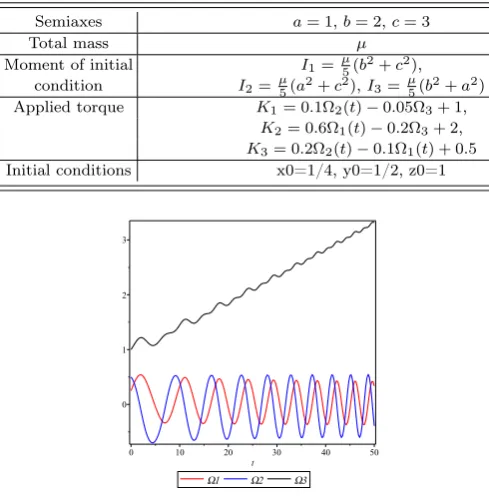
V. AN ASYMMETRIC TOP UNDER THE ACTION OF A GYROSTATIC MOMENT

FIG. 8. Ωprofiles of the case in Table VI

TABLE VII. Data for an asymmetric top under the action of a gyrostatic moment

Semiaxes a= 1,b= 2,c= 3

Total mass µ

Moment of initial I1= µ₅(b2+c2),

condition I2=µ₅(a2+c2),I3=µ₅(b2+a2)

Applied torque K1= 0.1Ω2(t)−0.05Ω3+ 1,

K2= 0.6Ω1(t)−0.2Ω3+ 2,

K3= 0.2Ω2(t)−0.1Ω1(t) + 0.5

Initial conditions x0=1/4, y0=1/2, z0=1

FIG. 9. Ωprofiles of the case in Table VII

velocitiy, the code could provide solutions without any difficulty. The data is presented in Table VII below.

The results are shown in Fig.9 below.

If we only change one semiaxes, namely c = k,k = 1, , 2, 3, 4, 5and keep all the others unchanged, then the results will be as follows, shown in Figures below, namely 10, 11 and 12.

VI. THERMODYNAMICAL CONSIDERATION OF ROTATING BODY

The above numerical studies show that longer axes of the rigid body are sensitive to any change of the torque

FIG. 10. Ω1 profiles withc=k,k= 1, , 2, 3, 4, 5

FIG. 11. Ω2 profiles withc=k,k= 1, , 2, 3, 4, 5

FIG. 12. Ω3 profiles withc=k,k= 1, , 2, 3, 4, 5

and that little variation leads to a dramatic change in the rotation velocity. In other words, the maximum mo-ment of inertia is the key factor in controlling rigid body rotation. Rotation about the maximum principal mo-ment of inertia represents the minimum possible kinetic energy for a given angular momentum that a system can possibly have.

S=S(Ein) =S(E−M2/(2I)), whereE is total energy, M is moment and I is moment of inertia. Because the body is a closed system, thus its total energy and an-gular momentum are conserved, and hence the entropy must have the maximum value possible for the givenM and E. Therefore, the equilibrium rotation of the body takes place about the axis with respect to which the mo-ment of inertia has the greatest possible value17_{. This is} called the principle of maximum moment of inertia of the rotating body.

VII. CONCLUSIONS

In conclusion, the moment of inertia is the key factor involved in controlling rigid body rotation17. Proper design of the body shape can achieve the desired perfor-mance of a top. The comparison confirmed that Tsiotras and Longuski’s results13 _{were highly accurate. For ease} of teaching and research, we have written a Maple code to find a solution for the Euler equations. The provided Maple code can be used generally to solve any problem related to Euler’s equations, while, importantly, it is also simple and user-friendly.

Availability of data: The data that supports the findings of this study is available from the corresponding author, upon reasonable request.

Conflict of interest: The author declares that he/she has no known competing financial interests or personal relationships that may have influenced the work reported in this paper.

B.-H. Sun: Conceptualization, Methodology, Formu-lations, Formal analysis, Funding acquisition, Investiga-tion, Writing Original draft preparaInvestiga-tion, Writing, Re-viewing and Editing, and all relevant associated works.

1_{Routh E.J., A treatise on the dynamics of a system of rigid} bod-ies, Macmillan, London (1877)

2_{Whittaker, E.T., A Treatise on the Analytical Dynamics of}

Par-ticles and Rigid Bodies, 4th ed., Cambridge University Press (1952)

3_{Kovalevskaya, S., Sur le probléme de la rotation d’un corps solide} autour d’un point fixe, Acta Mathematica (in French), 12:177-232 (1889)

4_{Synge, J.L., Classical Dynamics. In: Handbuch der Physik,} vol. 3/1: Principles of Classical Mechanics and Field Theory. Springer-Verlag, Berlin (1960)

5_{Leimanis, E., The general problem of the motion of coupled rigid}

bodies about a fixed point, Springer, New York (1965)

6_{Magnus, K.K., Theorie und Anvendungen, Springer, New York} (1971)

7_{Landau, L.D., Lifshitz, E.M.: Mechanics, 3rd ed., Pergamon}

Press (1976)

8_{Wittenburg, J., Dynamics of systems of rigid bodies, B. G.}

Teub-ner, Stuttgart (1977)

9_{Arnold, V.I., Mathematical Methods of Classical Mechanics, 2nd} ed., Springer (1978)

10_{Goldstein, H., Classical Mechanics, 2nd ed., Addison-Wesley}

(1980)

11_{Kane, T A and Levinson, DA, Dynamics: Theory and}

Applica-tions, McGraw-Hill Publishing Co, New York, 1985.

12_{Tsiotras, P., and Longuski, J. M., A complex analytical}

solu-tion for the attitude mosolu-tion of a near-symmetric rigid body un-der body-fixed torques. Celest. Mech. Dyn. Astr., 51(3):281-301 (1991)

13_{Tsiotras, P., and Longuski, J. M. Analytical solution of Euler’s}

equations of motion for an asymmetric rigid body. J. Appl. Mech, 63(1):149-155 (1996)

14_{Ershkov, S. V., New exact solution of Euler’s equations (rigid} body dynamics) in the case of rotation over the fixed point, Arch. Appl. Mech.,84:385-389 (2014)

15_{Amer, T.S. and Abady, I.M., Solutions of Euler’s Dynamic}

E-quations for the Motion of a Rigid Body, Journal of Aerospace Engineering, Nonlinear Dyn. 89:1591-1609 (2017)

16_{Amer, T.S. and Abady, I.M., Solutions of Euler’s Dynamic}

E-quations for the Motion of a Rigid Body, Journal of Aerospace Engineering, 04017021-1 (2017)

17_{Landau, L.D. and Lifshitz, E.M., Statistical Physics, Part 1, 3rd}