SUPPLEMENTARY MATERIAL OF IEEE TCST
PAPER
Amritam Das
∗1, Martijn Princen
1, Mahnaz Shokpour Roudbari
2, Amol Khalate
2, Siep Weiland
1Abstract
The supplementary material contains three items: a) an academic example of the digital twin; b) the proof of Algorithm IV.1; c) the proof of theorem VI.1.
Index Terms
Inkjet Printing, Thermo-Fluidic Processes, Spatially Interconnected Systems, Soft Sensing, Optimal Control.
NOMENCLATURE ¯
h average convective heat transfer W/(m2◦C) ˙
Qr Radiation Heat transfer W
Emissivity−
µ ViscosityN s/m2
ρ Density Kg/m3
k Thermal conductivityW/(m·◦C)
Ai Surface aream2
Across Cross-sectional aream2
Ai−j Contact aream2
ci Specific heat capacity J/(kg◦C)
Dh Hydraulic diameter m
Fij View factor between surfaces −
h Heat transfer coefficient W/(m2◦C)
Hv Convective heat transfer coefficientW/◦C
Hd Conductive heat transfer coefficient W/◦C
li Length from center of mass to surface m
Lc Characteristic lengthm
mi Masskg
Pcross Perimeter of the cross-sectionm
R Thermal resistance◦C/W Ti Temperature ◦C
v velocity m/s
Bi Biot Number−
N u Nusselt number−
Re Reynolds Number −
1Eindhoven University of Technology, Department of Electrical Engineering, Control Systems group, P.O. Box 513, 5600 MB Eindhoven, The Netherlands.
E-mail:[email protected], [email protected], [email protected]
2Canon Production Printing B.V., Van der Grintenstraat 10, 5914 HH Venlo, The Netherlands. E-mail: [email protected],
I. ACADEMIC EXAMPLE OF DIGITAL TWIN
Figure 1 presents a simplified example to demonstrate the use of the graph-theoretic modeling approach.
(a) Cross-sectional Schemtics (b) Graph Structure
Fig. 1: Example of a thermo-fluidic process
Here, the liquid tankL1has a time-varying inflow ofQin(t)m3/s and outflow ofQr(t)m3/s. Every individual nozzleLn1,
Ln2,Ln3 has liquid outflow with a time-varying flow rateQni(t)m3/s,i∈ {1,2,3}.
A. Graph
There are six nodes; :={S1,S2,L1,Ln1,Ln2,Ln3}.
B. Topology
The adjacent matrixA∈R6×6 is defined as follows
A=
0 1 1 0 0 0 1 0 1 1 1 1 1 1 0 0 0 0 0 1 1 0 0 0 0 1 1 0 0 0 0 1 1 0 0 0
(1)
It is evident that the topology of Lni is identical for i = {1,2,3}. In other words, topologically, there is no difference in the interconnection between any of the three nozzles and the rest of the graph. This is a major advantage for building graph-theoretic model.
C. Node dynamics
The equations governing the thermo-fluidic processes consist of three kinds of thermal energy transfer. They are: 1) Conduction: Heat transfer within solid nodes or via contact between solid nodes.
2) Convection: Heat transfer between the solid and liquid nodes.
3) Advection: Heat transfer via bulk movement of the liquid from one channel to the other. In the following items, the thermo-fluidic processes are derived per node:
S1: Its temperature TS1 (◦C) is influenced by convection with L1 and conduction with S1 according to the following
equation of energy conservation
CS1
dTS1
dt =Hd,1(TS2−TS1) +Hv,1(TL1−TS1).
Substituting the expressions of Hd,1, Hv,1, one obtains
mS1cS1
dTS1
dt
| {z } T hermal storage
= 1
Rtot | {z } Conduction
(TS2−TS1) +
N uL1·kL1
DhL1
AS1−L1
| {z }
Convection
(TL1−TS1). (2)
Here, the equivalent thermal resistance is Rtot= AS1−lSS12kS1 +
lg AS1−S2kg +
lS2
AS1−S2kS2.
L1: Its temperature TL1 (◦C) is influenced by advection and convection according to the following equation of energy
conservation
CL1
dTL1
In other words,
mL1cL1
dTL1
dt
| {z } T hermal storage
=N uL1·kL1
DhL1
AS1−L1
| {z }
Convection
(TS1−TL1) +
N uL1·kL1
DhL1
AS2−L1
| {z }
Convection
(TS2−TL1)
+ρincin(Qr(t) +
3
X
i=1
Qni(t)
| {z }
Advection
(Tin−TL1)). (3)
Lni: For individual liquid nozzleLnii∈ {1,2,3}, the governing equation is identical. Hence, as an example, the governing
equation of temperatureTLni (◦C) for node Lni is
CLni
dTLni
dt =Hv,ni(TS2−TLni) +Ha,ni(t)(TL1−TLni).
mLnicLni
dTLni
dt
| {z }
T hermal storage
=N uLni·kLni
DhLni
AS2−Lni
| {z }
Convection
(TS2−TLni) +ρL1cL1Qni(t) | {z }
Advection
(TL1−TLni). (4)
To obtain the thermo-fluidic model of every individual nozzle, one simply has to repeat (4) by substituting the physical parameters with indexi∈ {1,2,3}.
S2: This node is connected with all of the other nodes. Similar toS1, it temperature,TS2(◦C), is governed by the following
equation of energy conservation:
CS2
dTS2
dt =Hd,1(TS1−TS2) +Hv,2(TL1−TS2) +
3
X
i=1
Hv,ni(TLni−TS2)
mS2cS2
dTS2
dt
| {z } T hermal storage
= 1
Rtot | {z } Conduction
(TS1−TS2) +
N uL1·kL1
DhL1
AS2−L1
| {z }
Convection
(TL1−TS2) + 3
X
i=1
N uLni·kLni
DhLni
AS2−Lni
| {z }
Convection
(TLni−TS2)
(5)
Remark I.1. By construction, modularity is a key attribute in the thermo-fluidic process. As the dynamics and topological interconnection of every individual nozzle is identical with respect to the entire graph, the digital twin simply requires repetition of identical models based on the number of nozzles. This is a crucial advantage of graph-theoretic framework in building digital twin.
D. State-space representation of a node
For example, forS1, the temperature evolution can be re-written in the following state-space form:
˙
TS1
wS1,S2
wS1,L1
qS1
=
(Hd,1+Hv,1)
CS1
Hd,1
CS1
Hv,1
CS1 1 0
1 0 0 0 0
1 0 0 0 0
0 0 0 0 0
TS1
vS1,S2
vS1,L1
pS1
,
vS1,S2
vS1,L1
=
0 0 1 0 0 0 0 1
wS1,S2
wS1,L1
wS2,S1
wL1,S1
, pS1=qS1. (6)
E. Interconnection Structure
The interconnection relation v= ¯M wis given below.
vS1,S2
vS1,L1
vS2,S1
vS2,L1
vS2,Ln1
vL1,S1
vL1,S2
vLni,S2
vLni,L1
| {z } v =
0 0 1 0 0 0 0 0 0 0 0 0 0 0 1 0 0 0 1 0 0 0 0 0 0 0 0 0 0 0 0 0 0 1 0 0 0 0 0 0 0 0 0 0 1 0 1 0 0 0 0 0 0 0 0 0 0 1 0 0 0 0 0 0 0 0 0 1 0 0 0 0 0 0 0 0 0 0 0 1 0
| {z }
¯ M
wS1,S2
wS1,L1
wS2,S1
wS2,L1
wS2,Ln1
wL1,S1
wL1,S2
wL1,Lni
wLni,S2
| {z } w
(7)
For brevity, only one nozzle, Lni, is considered and it can be repeated for i ∈ {1,2,3}. This is again a major advantage
F. Determining the representationI
Now one can easily build the representationI by stacking all the signals:
˙
TS1(t)
˙
TS2(t)
˙
TL1(t)
˙
TLni(t) =
−(Hd,1+Hv,1)
CS1 0 0 0
0 −Hd,1+Hv,2+Hv,n1
CS2 0 0
0 0 −Hv,1+Hv,2
CL1 0
0 0 0 −Hv,ni
CLni
| {z }
Axx
TS1(t)
TS2(t)
TL1(t)
TLni(t) +
1 0 0 0 0 1 0 0 0 0 1 0 0 0 0 1
| {z }
Bxp
p(t)
+
Hd,1
CS1
Hv,1
CS1 0 0 0 0 0 0 0 0 0
0 0 Hd,1
CS2
Hv,2
CS2
Hv,n1
CS2 1
CS2 0 0 0 0 0
0 0 0 0 0 0 Hv,1
CL1
Hv,2
CL1 0 0 0
0 0 0 0 0 0 0 0 Hv,ni
CLni 0
1 CLni
| {z }
Bxv
v(t), (8)
q(t) =
0 0 0 0
0 0 0 0
0 0 −ρL1cL1
CL1 0
0 0 0 −ρL1cL1
CLni
| {z }
Cqx
TS1(t)
TS2(t)
TL1(t)
TLni(t) +
0 0 0 0 0 0 0 0 0 0 0
0 0 0 0 0 0 0 0 0 0 0
0 0 0 0 0 0 0 0 0 0 0
0 0 0 0 0 0 0 0 0 ρL1cL1
CLni 0
| {z }
Dqv
v(t), (9)
w(t) =
1 0 0 0 1 0 0 0 0 1 0 0 0 1 0 0 0 1 0 0 0 0 1 0 0 0 1 0 0 0 1 0 0 0 0 1 0 0 0 0 0 0 0 0
| {z }
Cwx
TS1(t)
TS2(t)
TL1(t)
TLni(t)
, (10)
y(t) =
0 0 0 1
| {z } Cyx
TS1(t)
TS2(t)
TL1(t)
TLni(t)
, (11)
p(t) =
1 0 0 0
0 1 0 0
0 0 Qr(t) +
3
P
i=1
Qni(t) 0
0 0 0 Qni(t)
| {z }
¯ Θ(t)
q(t). (12)
II. PROOF OF ALGORITHM IV.1
Proof: Consider a class of stable, second-order, single-input-single-output systems that has the following representation:
z(n+ 1) =Asz(n) +Bsw(n),
y(n) =Csz(n). (13)
Here, forn∈N∪ {0},z(n)∈R2 is a vector with two internal states andw(n)∈Ris the applied impulsive input. The output signaly(n)∈Ris modeled as (14).
y(n) =αe−ζnTssin(ωnT
s+φ) +γ; n∈N. (14)
A. Step 1: Determining the poles
The first task is to find an estimate of the state matrix As∈R2×2. To this end, the Hankel matrix is constructed using the data {sn, n∈N[1,N]} as follows:
H =
s1 . . . sL−1 sL
s2 . . . . sL sL+2
..
. . .. ... ...
sN−L . . . . sN−2 sN−1
sN−L+1 . . . sN−1 sN
=N−L+1L,
where, the observability matrix N−L+1 and the reachability matrixL are defined as
L :=
Bs AsBs · · · ALs−1Bs
,N−L+1:=
Cs
CsAs
.. .
CsANs−L
.
Remark II.1. (shift property of observability matrix)
1N−L+1As=2N−L+1,
where, 1
N−L+1=
Cs
CsAs
.. .
CsANs−L−1
and2
N−L+1=
CsAs
.. .
CsANs−L
.
As, we are interested in a second order system, let the optimal 2-rank approximation of the Hankel H be given by
H≈UΣVH, Σ :=diag(σ1, σ2), σ1, σ2>0.
In other words,
H ≈ UΣ12
| {z }
N−L+1
Σ12VH
| {z }
L
.
Now, using the shift property we obtain:
˜
As= Σ−
1
2U1†U2Σ 1 2,
whereA˜s=T−1AsT for an unknown matrixT. As the poles of the system does not change of under similarity transformation,
the two poles of As are found by solving the eigen valueρk and right eigen vector vk,k= 1,2:
( ˜As−ρk)vk= 0
B. Determine ω and ζ
Using the system poles, we find the frequencyω and the dampingζ as follows:
• Natural Frequency: ω=Im(lnρk), k= 1 or 2.
C. Determine α,φ, and γ
The amplitude α, the phaseφand the shiftγ are found by reconstructing the signalsn using computed values of ω,ζ. In
particular:
y(n) =αe−ζnTssin(ωnT
s+φ) +γ= (a+jb)ej(ω+jζ)nTs+ (a+jb)∗e−j(ω−jζ)nTs+γ.
=a
ej(ω+jζ)nTs+e−j(ω−jζ)nTs
+jb
ej(ω+jζ)nTs−e−j(ω−jζ)nTs
+γ. (15)
Here, a = α2sinφ and a = α2cosφ are the unknowns coefficients and γ is the unknown offset. Using the data at samples
{0,· · ·, N−1}, the unknowns can be found by solving the following linear equations:
s=Γx, (16)
Here, the unknowns are x := col(a, b, γ), s := col(s1,· · ·, sN) is the data. Moreover the matrix is defined as Γ :=
col
(ej(ω+jζ)nTs+e−j(ω−jζ)nTs) j(ej(ω+jζ)nTs−e−j(ω−jζ)nTs) 1
n∈N[1,N]
depends on ω and ζ, and . An unbiased
minimum variance solution of (16),xˆ:=col(ˆa,ˆb,γˆ), accepts the following analytic expression:
ˆ
x= (ΓHΓ)−1ΓHs. (17)
Using computed ˆx, the amplitude (α) and phase (φ) of the signal (14) are computed as follows:
• Amplitude: α= 2 q
Re(ˆa+jˆb)2+Im(ˆa+jˆb)2.
• Phase : φ=Im(ln(ˆa+jˆb)).
• Offset : γ= ˆγ.
The computed values of α,ζ,ω,γ andφ parametrize and reconstruct the signaly(n)in (14).
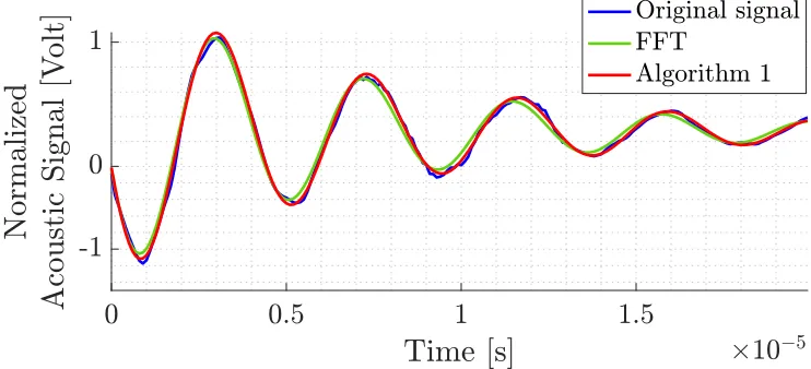
Remark II.2. We compare the developed algorithm against the conventional fast Fourier Transform (FFT) to judge the quality of reconstructing y(n). Figure 2 shows this comparison.
Fig. 2: Comparison of FFT and proposed algorithm to reconstruct y(n).
In Table I, the estimated key parameters are compared. In spite of a little larger computational time, due to increased accuracy, the proposed algorithm is preferred over FFT.
Table I: Key Parameters from the FFT, and Algorithm IV.1
Method ω α ζ φ γ time
(Mrad/s) (Volt) (-) (rad) (Volt) (s)
FFT 0.1475 166.49 0.0135 -2.8561 -0.8530 0.006
III. PROOF OF THEOREM VI.1
Proof: Regarding the presented tracking control problem, asymptotic stability is understood with respect to the following non-autonomous error system:
x((k+ 1)td)−xr
= ˜A(ktd)
x(ktd)−xr
+ ˜B(ktd)
uh(ktd)−ur(ktd)
. (18)
The asymptotic stability of the (18) in closed-loop amounts to verifying whether there exists δ >0 such that lim
k→∞||x(ktd)−
xr||= 0for all initial condition ||x(0)−xr||< δ while uh(kt
d)is applied by solving the MPC problem. To this end, using
Lyapunov theory (c.f. [1]), we show that the MPC cost functionalJ(k,·,·)at instantk, once substituted with unique minimizer ¯
x∗(k) :=col(x∗1|k,· · ·x∗N|k)andu¯h∗
k :={u h∗
0|k,· · ·, u h∗
N−1|k}, is a candidate Lyapunov function.
It is now possible to construct an input and state trajectory x¯f(k+ 1),u¯f(k+ 1) such that the MPC problem at timek+ 1 is feasible (not necessarily optimal) with costJf(k+ 1,x¯f(k+ 1),u¯f(k+ 1)). Here,
¯
xf(k+ 1) =col
x∗2|k,· · ·xN∗|k, xfN|k+1
,
¯
uf(k+ 1) =col
uh1|∗k,· · ·uhN∗−1|k, ufN−1|k+1
,
where, xf N|k+1, u
f
N−1|k+1 are future state and input to be determined by MPC at iteration k+ 1. Similar to the dual mode
formulation as proposed in [2], we construct the predicted terminal input at time stepk+ 1as a stabilizing state feedback law for (18). In other words,
(xfN|k+1−xr) =
˜
AN|k+ ˜BN|kKk
(x∗N|k−xr).
ufN−1|k+1=Kk(x∗N|k−x r) +ur
N|k.
Owing to the convexity and positivity of the objective function, for proving stability, it is sufficient to show that the feasible cost functional is contractive over time samples. In other words,
Jf(k+ 1,x¯f(k+ 1),u¯f(k+ 1))< J(k,x¯∗(k),u¯h∗(k)) Substituting the respective expressions, we obtain
Jf(k+ 1,x¯f(k+ 1),u¯f(k+ 1))−J(k,x¯∗(k),u¯h∗(k)) =−||x0|k−xr||2Q− ||u
h
0|k−u r
0|k||
2
R0|k− ||x ∗
N|k−x r||2
Pk +||x∗N|k−xr||2
Q+||Kk(x∗N|k−x r)||2
RN|k+||(AN|k+BN|kKk)(x ∗
N|k−x r)||2
Pk. (19)
Since the first two terms in the RHS of (19) is negative, we require to satisfy the following inequality for the contraction of the cost functional:
( ˜AN|k+ ˜BN|kKk)>Pk( ˜AN|k+ ˜BN|kKk)−Pk4−Q−Kk>RN|kKk, Pk 0
Using changes of variables Xk =Pk−1 andYk =KkPk−1 and using the rule of Schur complement we obtain the following
LMI:
−Xk 0 A˜N|kXk+ ˜BN|kYk 0
0 −R−N1|k Yk 0
( ˜AN|kXk+ ˜BN|kYk)> Yk> −Xk Xk
0 0 Xk −Q−1
4
0, Xk 0.
The corresponding control input uf
N−1|k+1 = Kk(x∗N|k−x r) +ur
N|k should also be an admissible control action. In other
words, uf
N−1|k+1 should satisfy the following constraint:
EN|k(Kk(x∗N|k−x r) +ur
N|k)< b
This amounts to the following terminal constraint on xN|k:
EN|kKkxN|k< b−urN|k+EN|kKkxr
REFERENCES
[1] F. Blanchini, “Set invariance in control,”Automatica, vol. 35, no. 11, pp. 1747 – 1767, 1999. [Online]. Available: http://www.sciencedirect.com/science/ article/pii/S0005109899001132