Network Simplification Preserving Bandwidth and
Routing Capabilities
Sergey I. Nikolenko
∗†, Kirill Kogan
‡, Antonio Fern´andez Anta
‡ ∗Steklov Institute of Mathematics at St. Petersburg,†National Research University Higher School of Economics, St. Petersburg ‡IMDEA Networks Institute, Madrid
Abstract—We introduce structural transformations that al-low simplifying a given network while preserving its original “bandwidth” and “routing” capabilities, transparently to specific allocations. We minimize a certain objective such as the aggregate capacity of network links, number of nodes, or number of links, in such a way that all the bandwidth that could be routed in the original network can also be routed in the reduced one. This improves cost-efficiency for both inter- and intra-datacenter connections and simplifies network management. We also identify a fundamental tradeoff between extra added capacity and sim-plicity of representation for a given network. Our analytic results are supported by extensive simulation results on hundreds of real network topologies. One result is that by adding 10-30% extra capacity to evaluated real-world networks one can simplify them down to a star topology with a single switch, while all routing and bandwidth allocation decisions on the simplified topology can be mapped back to the original network. This is an important step towards simplifying network management via a reduced virtualized network infrastructure.
I. INTRODUCTION
Network infrastructure is an expensive resource that requires complex management. Network providers are often unable to fully leverage this huge investment. To simplify network man-agement, one can propose to represent the original network with a simpler/cheaper network that still implements specific properties of the original. Usually, there is a tradeoff between the simplicity of network representations and efficient reuse of the underlying infrastructure.
There have been attempts to virtualize specific network architectures, optimizing various objectives [1], [2], but there is no well-understood process to get a simplified representation of a network while preserving its “bandwidth” and “routing” capabilities. This work is a first step in this direction. Pre-serving network capabilities allows to operate services on the simpler representation transparently from the physical infras-tructure. In addition, understanding the constraints of a given network shows which resources need additional investments.
The first problem we explore in this work (Section II) is capacity planning, by which we mean minimizing the aggregate capacity of the links in a network while maintaining its original topology. Since different coexisting applications can use bandwidth allocation methods that optimize different objectives (e.g., aiming for shortest, cheapest, or load-balanced traffic over several paths), we do not assume any knowledge about bandwidth allocation methods and routing for inter-connecting sources and destinations. In fact, the resulting set
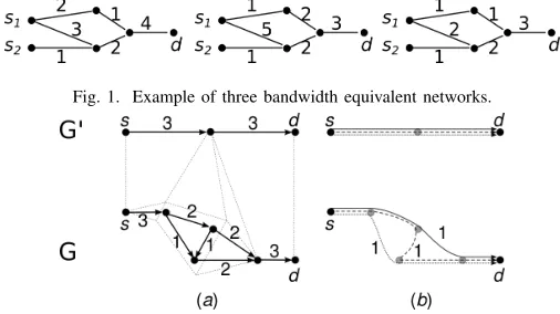
Fig. 1. Example of three bandwidth equivalent networks.
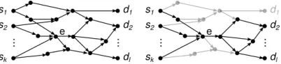
Fig. 2. Bandwidth equivalence: (a) two equivalent graphs, (b) a bandwidth allocation onG0 with three routes of bandwidth1maps toG.
of link capacities must allow for any bandwidth allocation and routing the original did, a property we call bandwidth equivalence. For a simple example, the three networks on Fig. 1 are all bandwidth equivalent: any set of routes from s1 and s2 to d that satisfies capacity constraints shown on
the edges of one of the graphs will also satisfy them in the two others. However, the graphs have very different total capacities, and the result of capacity planning for all three networks on Fig. 1 should be the network on the right, which has minimal aggregate capacity and cannot be reduced further. Useful applications of capacity planning include various WAN optimizations for interconnected geo-distributed data-centers, where WAN links are extremely expensive [3], [4].
Fig. 3. Examples: Different maximal flows lead to different total capacity.
is a strong property. In Section III, we explore additional transformations that relax it, allowing further simplifications: even without a 1-to-1 mapping between bandwidth allocations, one can guarantee that any bandwidth routed from sources to destinations in one network is also feasible in the other. Finally, in Section IV we explore further possibilities. First we show an instance of the well-known Braess’ Paradox in our context: removing a link from a network may not affect its capabilities negatively but rather allow to drastically reduce its size. Second, we find a fundamental tradeoff between additional network topology simplification and extra capacity that would be required to achieve it.
Our analytic results are supported by a solid simulation study on real network topologies (Section V) that confirm that proposed transformations are applicable in practice. In particular, adding 10-30% extra capacity to real world net-works allows to simplify them to a star topology (connecting sources and destinations through a single switch), where all routing and bandwidth allocation decisions can be mapped back to the original network. This represents an important step towards improving the management of virtualized network infrastructure. We conclude the paper with Section VII, where we discuss further extensions.
II. CAPACITYPLANNING
In this section, we consider capacity minimization for a given network with a predefined set of sources and destina-tions, aiming to minimize capacity transparently to bandwidth allocation methods. Informally, a bandwidth allocation is a set of paths between sources and destinations, with bandwidth values assigned to them, that satisfy link capacity constraints. Themaximal network flowbetween sources and destinations could be used to find a potential reduction in required network capacities. Clearly, if we find maximal flow values for every link we can safely reduce original capacities to these values: there is no way to allocate more bandwidth between sources and destinations through each specific link. Unfortunately, two different instances of maximal network flow can result in different total network capacity. For a very simple example, observe on Fig. 3 (left) that the maximal flow through the top path leads to total capacity 3, and the max flow through the bottom path leads to total capacity 4; this can add up to arbitrarily large discrepancies (Fig. 3, right). Besides, ob-jectives of various bandwidth allocation methods can extend beyond optimal reuse of underlying network infrastructure and can be application-specific. For instance, one objective can be to allocate bandwidth along a “shortest” path for low-latency traffic, while using the “cheapest” for another; both objectives can be implemented simultaneously within the same network by different applications. All this has led us to the formal notion of bandwidth equivalencebetween two networks.
A. Bandwidth Equivalence
As a network interconnect, we consider a weighted directed network G= (V, E, w, S, D) without self-loops, where V is a set of vertices, E is a set of edges among them, and w : E → R+ is a weight function that represents an available
capacities on edges. In addition some vertices inV are marked as sources S ⊂V anddestinations D ⊂V. We assume that source vertices do not have incoming edges and destination vertices do not have outgoing edges1.
We begin with the notion of bandwidth allocation; the intu-ition is to define a set of routing paths together with specific bandwidths allocated along these paths. Namely, abandwidth allocation A = (P, f) on a network G= (V, E, w, S, D) is a set of edge-simple paths P ={p1, . . . , pk} and a function f :P →R+ such that:
(1) ∀i∈[1, k], pathpi= (v1, . . . , vli)starts at a source vertex
v1∈S and ends at a destination vertex vli∈D;
(2) f(pi)≥0 for everyi(nonnegativity); (3) for every e ∈ E, P
p∈P:e∈pf(p) ≤ w(e) (capacity constraints).
Note that paths in a bandwidth allocation can contain loops (but cannot cross the same edge twice).2
Two weighted networks G = (V, E, w, S, D) and G0 = (V, E, w0, S, D) with the same graph structure but possibly different weight functions w and w0 are called bandwidth equivalent, denoted G'G0, if every bandwidth allocationA on network Gis also a bandwidth allocation on network G0, and vice versa. This definition does not depend on a specific objective such as minimizing the number of edges or nodes.
For a simple example of bandwidth equivalence, see Fig. 1: all three networks are bandwidth equivalent and can support the same bandwidth allocations. However, the network on the right of Fig. 1 is special: one cannot further reduce the capacity of any edge in this network without violating bandwidth equivalence. We call a network G∗ = (V, E, w∗, S, D) a
minimal bandwidth networkif, for every networkG= (V, E, w, S, D) such that G' G∗, it holds that w∗(e)≤w(e) for everye∈E. Note that this definition uses a specific objective, the total capacity of all edgesP
e∈Ew(e).
B. Existence and Uniqueness of Minimal Bandwidth Networks
The first problem we consider is to find the minimal bandwidth networkG∗ in the bandwidth equivalence class of a given networkG. Note that if a minimal bandwidth network equivalent to a given G exists and is unique, it obviously also minimizes the total capacity of all edges P
e∈Ew∗(e); however, it is not obvious that it exists at all. Fortunately, we can provide a constructive definition: an explicit algorithm to construct minimal bandwidth networks. Given a network G, thebrute force (BF) algorithm to findG∗ works as follows:
1If they do, we can simply replace an internal source vertexsby an internal
nodevsand a new sources0linked to that internal nodevswith an infinite
capacity edge, and similarly for an internal destination vertex.
2The notion of bandwidth allocation is similar in spirit to flow
Fig. 4. The subgraphGe used in the DAG-OPT algorithm.
• for every subgraphG0⊆Gwith induced edge capacities, compute max-flowfG0 from sourcesSto destinationsD; • for every edge e∈E, set its capacity inG∗ to the max-imum of all flow values, i.e.,w∗(e) = maxG0⊆GfG0(e).
Theorem 1. For every input network, the BF algorithm computes a minimal bandwidth network G∗ that is unique.
C. Polynomial Time Algorithm for DAGs
The BF algorithm is obviously exponential since it includes enumerating all subgraphs. We show now an algorithm that finds the minimal bandwidth network in polynomial time if the graph has no cycles; since we restrict the algorithm to directed acyclic graphs (DAGs), we call itDAG-OPT. To find a minimal bandwidth network equivalent to a DAGG= (V, E, w, S, D), DAG-OPT proceeds as follows:
(1) sort vertices of Gin topological order: u≤v if Ghas a path fromutov (here we use the fact thatGis a DAG); (2) for every edgee= (u, v):
(i) consider the subgraphGeofGinduced by the vertex setVewhich contains vertices comparable touin the topological order:Ve={v0 ∈V | v0 ≤u} ∪ {v0 ∈ V |v0≥v};
(ii) find a maximal flow fG∗
e on Ge from sources to
destinations;
(iii) set the final capacityw∗(e)to the flow throughein this maximal flow,w∗(e) =fG∗
e(e).
This algorithm is illustrated in Fig. 4. Essentially, to find the optimal capacity for an edgeewe remove all vertices and edges that are not connected to paths througheand solve the maximal flow problem on the resulting subgraph, which can be done in O(|V||E|)time [5].
Theorem 2. The algorithm DAG-OPT outputs the minimal bandwidth network G∗ equivalent to a given network (DAG)
Gin timeO(|V||E|2).
D. Efficient Local Heuristic for Bandwidth Equivalence
We now present a local heuristic that, although it does not find the minimal bandwidth graph in general, produces good results in practice (see Section V). We also show that this heuristic is optimal on graphs whose undirected version is a forest, and, unlike DAG-OPT, it can be applied to graphs with cycles. Moreover, this algorithm, calledWPP, has computational complexityO(|E|+|V|log|V|), as opposed to O(|V||E|2)of DAG-OPT.
Consider a graphG= (V, E, w, S, D); the goal is to reduce its total capacityP
e∈Ew(e). Let us denote the total capacity of the incoming and outgoing links of a vertex v by Iv and
Algorithm 1 Algorithm WPP(G) 1: N←V
2: whileN6=∅do
3: Choosev∈N: min{Iv,Ov}= minu∈N{Iu,Ou}
4: Apply WP to all edgeseincident tov
5: N←N\ {v}
Ov, respectively; we also denoteIe=Iu,Oe=Ov, fore= (u, v)∈E.
The algorithm is based on a local capacity adjustment that we call weight propagation (WP). WP uses a simple obser-vation that an edge e ∈ E cannot transmit more bandwidth than Ie or Oe.3 To apply WP to an edge e ∈ E is to set w(e) ← min{w(e),Ie,Oe}; this yields a new graph which is bandwidth equivalent to G. If w(e) > min{Ie,Oe}, by applying WP to ewe reduce its capacity and hence the total capacity. WPP applies WP to the edges until no edgeesatisfies w(e) > min{Ie,Oe}. To bound the complexity, we need to bound the number of WP applications, which is done by carefully choosing the edges on which applying WP next. WPP is presented in Algorithm 1: it processes the nodes ofG, chooses on each iteration an unprocessed nodevwith minimal min{Iv,Ov} and applies WP to all edges incident tov.
As described, WPP runs for |V| iterations, and the WP process is applied to every edge at most twice. The node v for each iteration can be chosen with a strict Fibonacci heap [6], which is created with complexity O(|V|), but in which finding the minimum and decreasing a value takes constant time, and deleting the minimum takesO(log|V|)time. Hence, WPP has time complexityO(|E|+|V|log|V|). It also holds that once WPP is completed, all edges of the resulting graph G0= (V, E, w0, S, D)satisfyw0(e)≤min{I0
e,Oe0}.
Theorem 3. The algorithm WPP, after processing graph
G= (V, E, w, S, D), outputs a graphG0 = (V, E, w0, S, D)
such that G0 ' G and, ∀e ∈ E, w0(e) ≤ w(e) and
w0(e)≤min{I0
e,Oe0}, in timeO(|E|+|V|log|V|).
Observe that we do not claim that the graphG0 obtained by WPP is the minimal bandwidth graph equivalent toG, because this is not always the case: WPP is local, and it is unable to process far-reaching dependencies between not immediately connected parts of the graph. For a formal counterexample, see Fig. 5, where an edge with capacity 2 can never route bandwidth larger than1(due to the bridge to destination with capacity1), but WP operations are inapplicable because locally a bandwidth of2can be pushed further, and the bottleneck is two steps away. Fig. 5b shows that in this way we can achieve an arbitrarily bad approximation ratio between WPP and the optimal total capacity: each of thekedges with capacitykcan be reduced to capacity1in the minimal bandwidth graph, but will not be reduced at all by WPP, so the total capacity of the graph output by WPP isk2+ 2k+ 1vs.3k+ 1in the minimal
bandwidth graph. This example shows that algorithm WPP is
3In this section, we assume that every source shasI
s =∞and every
destinationdhasOd=∞; recall that sources have no incoming links and
Fig. 5. Counterexamples for the optimality of WPP: (a) simple example; (b) arbitrary approximation ratio.
not guaranteed to find the minimal bandwidth graph in general. However, first, as we will see in Section V, WPP achieves excellent results in practice. And second, in the common special case of a forest, WPP is optimal.
Theorem 4. LetG= (V, E, w, S, D)be a graph such that its undirected version is a forest. Then WPP applied toGoutputs the minimal bandwidth network G∗ equivalent toG.
III. NETWORKTOPOLOGYTRANSFORMATIONS We have shown how to reduce the total capacity of a network while preserving its original topology. This is required in some problems (e.g., capacity planning) but in case of network simplification/virtualization the objective is different: simpler network management. The idea of network topology transformations that we introduce in this section is to find, for a networkG, a simpler networkG0that can satisfy exactly the same bandwidth requests as G. SinceG0is simpler, the feasi-bility of bandwidth requests can be checked more efficiently. Such transformations can be used to simplify management, representing a complex network with a much simpler structure which is easier to manage/configure.
In this section we explore this idea at two levels. First, we look for a network G0 that can be used to simplify routing: routing is done in the simple networkG0, and the routes found are mapped 1-to-1 to routes in the original networkG. Second, we show that one can simplify the network even further at the cost of losing the 1-to-1 correspondence between routes, while still preserving the feasibility property. We have summarized the proposed transformations in Figure 6.
A. Routing Equivalent Transformations
We begin by defining the concept of routing equivalence, which can be viewed as an extension of bandwidth equiv-alence. Intuitively, two networks are routing equivalent if they can carry the exact same set of bandwidth allocations (as defined in Section II-A), even though they may have a completely different structure. Formally, two networks G = (V, E, w, S, D) and G0 = (V0, E0, w0, S, D) with the same set of sources and destinations are routing equivalentif there is a one-to-one mapping g : PathG(S, D)→PathG0(S, D)4 between paths from sources to destinations on GandG0 that preserves bandwidth allocations. I.e.,
4Path
G(A, B)is the set of paths in networkG= (V, E)that begin in A⊆V and end inB⊆V.
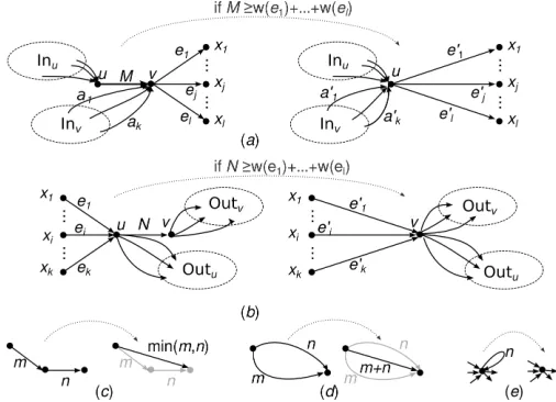
Fig. 6. Topology transformations: (a) shrinking non-bottleneck incoming edge; (b) shrinking non-bottleneck outgoing edge; (c) merging parallel edges; (d) removing self-loops; (e) path of length 2.
(1) for every bandwidth allocation A = ({p1, . . . , pk}, f) on network G, A0 = ({g(p1), . . . , g(pk)}, f0), where f0(g(p)) =f(p), is a bandwidth allocation on G0; (2) and vice versa, for every bandwidth allocation A0 =
({p0
1, . . . , p0k}, f0) on network G0, A = ({g−
1(p0
1), . . . ,
g−1(p0
k)}, f), where f(p) = f
0(g(p)), is a bandwidth
allocation onG.
Our objective is to propose ways to transform a network Ginto a simpler routing equivalent networkG0. The transfor-mation process must also provide the functiong−1that maps any bandwidth allocation on the simple network G0 back to G. The proposed transformations are illustrated in Figure 6. They can be summarized in the following two heuristics.
1. Shrinking a non-bottleneck incoming edge. The most general form of this heuristic is shown on Fig. 6a. Consider an edge e = (u, v) such that u /∈ S, v /∈ D, and u 6= v.5
If e has capacity w(e) = M and its outgoing edges have aggregate capacityOv=Pej∈Outvw(ej)≤M, theneis not
a bottleneck in any bandwidth allocation and can be shrunk into a single node u. This means that node v and edge e disappear, each edge ej = (v, xj) ∈ Outv is replaced by a new edge e0
j = (u, xj) with capacity w(e0j) = w(ej) = nj, and each edge ai = (y, v) ∈ Inv is replaced by a new edge a0i = (y, u) with capacity w(a0i) = w(ai). The func-tion g maps a path p = (. . . , e0, e, ej, . . .) ∈ PathG(S, D) into g(p) = (. . . , e0, e0j, . . .) Note that g is 1-to-1 since a path p0 = (. . . , e0, e0j, . . .) ∈ PathG0(S, D) is mapped to either g−1(p0) = (. . . , e0, e, e
j, . . .) (if e0 ∈ In(u)) or to g−1(p0) = (. . . , a
i, ej, . . .)(ife0=a0iis one of the new edges that replaced Inv). Fig. 6a illustrates this case, and Fig. 6c shows an important special case whenl= 1.
2.Shrinking a non-bottleneck outgoing edge. This heuristic is symmetric to the previous one, as shown in Fig. 6b, but with respect to the aggregate capacity of the edges incoming tou.
If Iu = Pj∈Inuw(ej) ≤ N the link e = (u, v) is shrunk into a single node v. The mapping function g is similar to the previous case. As before, Fig. 6c is a special case of this heuristic when k= 1.
Note that Transformations 1 and 2 reduce simultaneously the number of edges in the network, the number of vertices in the network, and the total capacity of all edges.
Theorem 5. The network G0 = (V0, E0, w0, S, D) obtained by applying Transformations 1 and 2 to a network G = (V, E, w, S, D)is routing equivalent toG.
B. Bandwidth Preserving Transformations
Transformations 1 and 2 proposed in the previous subsection produce routing equivalent simpler graphs. In this section, we introduce a relaxation of the routing equivalence property, called bandwidth-preserving routing transformation, allowing for even simpler graphs. Intuitively, the property that is guar-anteed by a bandwidth preserving routing transformation is that any feasible allocation in the derived graph G0 can be realized in graph G. The bad news is that the routes are not directly given by mappingg, since it is not 1-1 anymore. The good news is that this relaxed property allows to apply new graph transformations that in most cases allow to end up with a much simpler graph G0.
For two networks G= (V, E, w, S, D) andG0 = (V0, E0, w0, S, D) with the same set of sources and destinations, a
bandwidth-preserving routing transformationis a mappingg: PathG(S, D) → PathG0(S, D) between paths from sources to destinations on GandG0 that satisfies the following: (1) for every bandwidth allocation A = ({p1, . . . , pk}, f)
on network G, A0 = ({g(p1), . . . , g(pk)}, f0), where f0(g(p)) =P
q∈g−1(g(p))f(q), is a bandwidth allocation
on G0;
(2) for every bandwidth allocation A0 = ({p01, . . . , p0k}, f0) on network G0, there exists a function f : ∪k
i=1g− 1(p0
i)
→ R such that f0(p0) = Pp∈g−1(p0)f(p) and A = (∪k
i=1g−1(p0i), f)is a bandwidth allocation onG. We add the following two transformations.
3.Merge parallel edges. If there are two parallel edges with capacitiesmandnfrom vertexuto vertex v, we can replace (merge) them by one new edge fromutovwith total capacity m+n. This transformation is illustrated in Fig. 6d.
4.Remove self-loops. After some transformations, self-loops may arise in the graph; they can be simply removed (Fig. 6e). Figure 7b-g shows how the repetitive application of the above transformations can drastically simplify a graph.
Theorem 6. Transformations 3 and 4 are bandwidth preserv-ing routpreserv-ing transformations.
For the special case in which the initial graph G is a forest, it is easy to see that the graph G0 obtained with any bandwidth-preserving routing transformation g, is in fact routing equivalent. This follows since a path p0
i in G0 from s∈S tod∈D can only be the image of a unique path from s todinG, and henceg is 1-to-1.
Fig. 7. Example of Braess’ Paradox and the tradeoff between total capacity and topology optimization: (a) original graph; (b) graph with one edge capacity increased; Transformation 2 is applied to link(b, c); (c-g) further simplifications (dashed lines) lead to total collapse of the graph.
Observation 7. A bandwidth preserving routing transforma-tion applied to a forestG= (V, E, w, S, D)generates a graph
G0= (V0, E0, w0, S, D)that is routing equivalent toG.
IV. TRADEOFFS AND APARADOX
In the previous section we have proposed various transfor-mations that aim to reduce edge capacities and network topol-ogy as much as possible to simplify network management. Now, we explore the options we have with a network that cannot be further simplified with those transformations; we will see that sometimes there is yet more to be done.
We begin with a paradoxical network shown on Fig. 7a: the network allows to route bandwidth of 3 from s to d. None of the transformations proposed above can be used to simplify the network. Surprisingly, after removing one edge, the central edgee= (a, b)of capacity1, we can start a chain of transformations that lead to the trivial graph on Fig. 7g. Note that the bandwidth that can be sent from sto d in the network is not affected by the removal of edgeefrom Fig. 7a, so this is a bandwidth-preserving routing transformation. This phenomenon can be regarded as an instance of the well-known Braess’ Paradox [7], and it is worth to be studied further; e.g., is there an efficient algorithm for identifying edges that hinder simplification without any side benefits?
Starting again from a network that cannot be simplified with transformations shown above, we consider a fundamental tradeoff between network topology simplification and extra capacity required to achieve it. As a motivating example, see Fig. 7 again: the original graph Fig. 7a is irreducible, but if we increase the capacity of a single edge e0 = (b, c) by 1 (Fig. 7b), the graph again collapses to Fig. 7g.
a star graph). The problem can be posed in several versions: (a) given a capacity budget C, find the allocation of this capacity budget to edges of the input graph such that the resulting graph can be simplified as much as possible (in terms of the number of edges, number of vertices, or both) with bandwidth-preserving routing transformations; (b) what is the minimal total capacity that has to be added to the graph so that there exists a bandwidth-preserving routing transformation to a star graph. Both problems (a) and (b) are hard optimization problems. For Problem (a) we propose a local heuristic to find a reasonable tradeoff value: After repeatedly applying transformations from Section III, we are left with a graph where every edge is a bottleneck (and hence transformations 1 and 2 cannot be applied). We choose the best edge e to augment its capacity with the following greedy algorithm: (1) for every edgee∈E of graphG,
(i) find the minimal capacitywesuch that, by increasing its capacity tow(e) +we,estops being a bottleneck; (ii) repeatedly apply Transformations 1–4 from Sec-tion III to the graph obtained from G by setting w(e) ← w(e) + we, getting reduced bandwidth equivalent graphGe;
(iii) measure the resulting graph complexityC(Ge); (2) choose esuch that C(G)−C(Ge)
we is maximal.
Here one can use different graph complexity measures C(G) depending on the objectives, e.g., number of edges, number of vertices, their sum, and so on. To solve problem (b) this process has to be repeated until a star graph is obtained; these heuristics will be evaluated in the next section.
V. EVALUATION
In this section, we present experimental results generated by our heuristics. We have used graph topologies generated by the topobenchlibrary [8], [9] and by the networkxpython library. In particular, we have generated a number of bench-mark graphs in the following topologies: Fat Tree [10], a common topology of choice in modern data centers and high-performance computing; Jellyfish [11], [12], a recently proposed random topology for high throughput data centers;
VL2[13], a heterogeneous network structure proposed for data centers; SWDC ring topology [14] that connects nodes in a data center at random according to a distribution based on small-world networks;Dragonfly [15] that aims to reduce the network diameter by creating a virtual router out of a group of routers; powerlawcluster graph randomly generated with the Holme and Kim algorithm [16], which are random graphs of real world networks naturally arising in social networks and similar environments; hypercube regular topology [17] often used in high-performance computing.
Undirected unweighted topologies have been converted into directed acyclic graphs; we also assigned a capacity to every edge and labeled several first and last vertices in the chosen topological order as source and destination vertices. After this procedure, we obtained a collection of directed acyclic graphs that reflect various topologies suggested for modern
data centers. We have tested our algorithms across a wide variety of different generation parameters for each topology; the tables below reflect only some characteristic examples. An implementation of our algorithms together with sample topolo-gies that can be used to recreate Tables I and II can be found athttp://github.com/infocom2017anonymous/virtualization.
In the first experiment, we ran our capacity reduction algorithms, DAG-OPT which is optimal for directed acyclic graphs, and the approximation heuristic WPP, on the generated topologies. The results are shown in the WPP and DAG-OPT columns of Table I. Results show that in most cases, we are able to reduce the total graph capacity very significantly. (The figures on bold are reductions of at least 50%.)
The rest of Table I shows the results of our topology reduction heuristics. We show the routing equivalent and routing non-equivalent heuristics in three versions: starting from the original graph, starting from the WPP-reduced graph, and starting from the graph reduced by DAG-OPT. We see in Table I that for most topologies, the proposed heuristics are able to significantly reduce the graph topology, sometimes reducing the number of edges and vertices by a factor of5or more. Figures in bold show a reduction of at least 50%.
Finally, our most interesting results deal with the capacity vs. simplicity tradeoff as discussed in Section IV. In these experiments, we evaluate how much capacity we need to add to completely collapse the graph into a star graph. Table II shows numerical results; we show how much extra capacity is needed to collapse the graph in the two cases: with routing equivalent and routing non-equivalent transformations. Note that in most cases, the required extra capacity represents less than 35% of the total original capacity (shown in bold); the table also shows two cases (SWDC ring and Dragonfly) when the graph is collapsed with no extra capacity. Hence, our experiments let us conclude that network virtualization can be achieved in most currently used network topologies at a small cost.
VI. RELATEDWORK
Original graph Reduced Routing equivalent Routing non-equivalent
DAG Original WPP DAG-OPT Original WPP DAG-OPT Topology |V| |E| Capac. WPP OPT |V| |E| Capac. |V| |E| Capac. |V| |E| Capac. |V| |E| Capac. |V| |E| Capac. |V| |E| Capac. Fat Tree 330 2305 12670 9169 1780 207 2168 11807 202 2163 8672 61 2022 1546 177 1520 10802 201 1634 8649 53 349 1411
328 1389 7535 5258 5089 150 1195 6320 145 1190 4627 143 1188 4468 119 746 4958 143 913 4406 133 883 4124 Jellyfish 50 285 21721 20504 20504 36 256 21278 36 256 20205 36 256 20205 36 248 21278 36 248 20205 36 248 20205 60 374 28827 27258 27258 42 339 27873 42 339 26586 42 339 26586 41 320 27576 41 312 26297 41 312 26297 50 282 21795 20443 20443 36 257 21336 36 257 20110 36 257 20110 36 248 21300 36 236 19983 36 236 19983 VL2 67 212 1021 694 663 19 151 734 18 150 555 18 150 526 19 73 724 18 69 548 18 69 519 102 351 1725 1163 1163 27 260 1257 25 258 932 25 258 932 13 23 567 22 94 858 22 94 858
112 312 1604 883 883 21 209 1010 14 202 606 14 202 606 18 40 848 13 25 482 13 25 482
SWDC ring 42 105 6010 5132 5132 19 65 4592 19 65 4218 19 65 4218 17 50 4097 18 53 4066 18 53 4066 26 63 2658 2170 2170 11 31 2115 11 31 1896 11 31 1896 11 29 2115 11 29 1896 11 29 1896 18 38 752 486 486 5 8 533 5 8 402 5 8 402 5 6 533 5 6 402 5 6 402 Dragonfly 65 193 14091 12733 12660 39 149 12040 37 147 11059 37 147 11016 30 112 9630 32 114 9686 34 122 10120 Powerlaw 60 122 7937 2207 2181 22 68 5107 12 58 1605 13 59 1670 19 48 4052 12 27 1571 13 32 1636
110 220 16617 2138 2039 30 126 9782 13 109 1795 13 109 1696 29 95 9181 13 28 1773 12 27 1512
210 422 32758 4196 2999 48 244 18759 19 215 3122 15 211 2107 40 155 15507 19 57 2998 15 42 2021
Hypercube 138 472 37820 35201 35201 108 428 35164 104 424 32939 104 424 32939 107 418 34938 104 418 32939 104 418 32939 266 1049 83227 78565 78527 215 983 77922 203 971 73162 204 972 73253 213 968 77616 201 950 72781 202 953 72872 42 107 5955 5239 5185 22 70 4636 23 71 4514 23 71 4460 21 61 4401 23 66 4514 23 66 4460
TABLE I
EVALUATION RESULTS FOR CAPACITY PLANNING AND TOPOLOGY REDUCTION ALGORITHMS.
Original graph Routing equivalent Routing non-equivalent DAG No tradeoff Added Tradeoff No tradeoff Added Tradeoff Topology |V| |E| Capac. OPT |V| |E| Capac. capac. |V| |E| Capac. |V| |E| Capac. capac. |V| |E| Capac. Fat Tree 320 2281 12670 1780 61 2022 1546 916 12 1973 1296 53 349 1411 236 12 11 400
318 1363 7535 5089 143 1188 4468 3886 13 1058 3451 133 883 4124 1189 12 16 338
Jellyfish 40 260 21721 20504 36 256 20205 14708 12 232 17003 36 248 20205 7253 12 29 9656
50 347 28827 27258 42 339 26586 17213 12 309 22722 41 312 26297 9700 12 47 16103 60 433 34936 31403 48 421 30459 28769 11 384 25496 47 391 30245 11354 10 17 8381
VL2 57 189 1021 663 18 150 526 207 13 145 493 18 69 519 102 13 12 298
92 325 1725 1163 25 258 932 385 12 245 838 22 94 858 73 12 11 356
102 290 1604 883 14 202 606 142 11 199 585 13 25 482 31 11 10 214
SWDC ring 32 78 6010 5132 19 65 4218 999 10 56 3424 18 53 4066 596 9 19 2309
16 36 2658 2170 11 31 1896 126 10 30 1824 11 29 1896 126 10 25 1702 8 11 752 486 5 8 402 0 5 8 402 5 6 402 0 5 6 402 Dragonfly 55 165 14091 12660 37 147 11016 6023 11 121 8078 34 122 10120 1857 11 25 3619
Powerlaw 50 96 7937 2181 13 59 1670 221 10 56 1514 13 32 1636 221 10 22 1360
100 196 16617 2039 13 109 1696 0 13 109 1696 12 27 1512 0 12 27 1512
200 396 32758 2999 15 211 2107 335 10 206 1886 13 35 1866 331 10 21 1515
Hypercube 512 2304 189832 184774 442 2234 177182 234913 13 1805 119874 440 2218 176841 99767 13 26 7530
256 1024 83227 78527 204 972 73253 77254 11 779 48215 202 953 72872 26286 11 21 5470
32 80 5955 5185 23 71 4460 1513 11 59 3632 23 66 4460 503 11 24 2788
TABLE II
EVALUATION RESULTS FOR TRADING CAPACITY FOR SIMPLICITY:EXTRA CAPACITY NEEDED TO REDUCE THE GRAPH TO A STAR GRAPH.
VII. DISCUSSION ANDCONCLUSION
In this work we have shown how a network can be reduced to a much simpler network, where sensible management and routing decisions can be made. This is, however, only the first step towards a much more ambitious goal: represent the original network as a small virtual switch, where a richer set of decisions (e.g., scheduling) can be made and mapped to operations in the physical network.
Acknoledgments: We thank the anonymous reviewers for their insightful comments. The work of Antonio Fern´andez Anta is supported in part by Ministerio de Economia y Com-petitividad grant TEC2014-55713-R, Regional Government of Madrid (CM) grant Cloud4BigData (S2013/ICE-2894, co-funded by FSE & FEDER), NSF of China grant 61520106005. The work of Sergey Nikolenko was partially supported by the Government of the Russian Federation grant 14.Z50.31.0030 and Presidential Grant for Young Ph.D. MK-7287.2016.1.
REFERENCES
[1] M. Alizadeh, S. Yang, M. Sharif, S. Katti, N. McKeown, B. Prabhakar, and S. Shenker, “pfabric: minimal near-optimal datacenter transport,” in SIGCOMM, 2013, pp. 435–446.
[2] N. Kang, Z. Liu, J. Rexford, and D. Walker, “Optimizing the ”one big switch” abstraction in software-defined networks,” inCoNEXT, 2013, pp. 13–24.
[3] C. Hong, S. Kandula, R. Mahajan, M. Zhang, V. Gill, M. Nanduri, and R. Wattenhofer, “Achieving high utilization with software-driven WAN,” inSIGCOMM, 2013, pp. 15–26.
[4] S. Jain, A. Kumar, S. Mandal, J. Ong, L. Poutievski, A. Singh, S. Venkata, J. Wanderer, J. Zhou, M. Zhu, J. Zolla, U. H¨olzle, S. Stuart, and A. Vahdat, “B4: experience with a globally-deployed software defined wan,” inSIGCOMM, 2013, pp. 3–14.
[5] J. B. Orlin, “Max flows in o(nm) time, or better,” inSTOC, 2013, pp. 765–774.
[6] G. S. Brodal, G. Lagogiannis, and R. E. Tarjan, “Strict fibonacci heaps,” inProc. 44th Annual ACM Symposium on Theory of Computing, 2012, pp. 1177–1184.
[7] R. Steinberg and W. I. Zangwill, “The prevalence of braess’ paradox,” Transportation Science, vol. 17, no. 3, pp. 301–318, 1983.
[8] S. A. Jyothi, A. Singla, P. B. Godfrey, and A. Kolla, “Measuring and Understanding Throughput of Network Topologies,” Tech. Rep., 2014, http://arxiv.org/abs/1402.2531.
[9] “Topobench,” https://github.com/ankitsingla/topobench.
[10] C. Leiserson, “Fat-trees: Universal networks for hardware-efficient su-percomputing,” Computers, IEEE Transactions on, vol. C-34, no. 10, pp. 892–901, Oct 1985.
[11] A. Singla, C. Hong, L. Popa, and P. B. Godfrey, “Jellyfish: Networking data centers randomly,” inNSDI, 2012, pp. 225–238.
[12] A. Singla, P. B. Godfrey, and A. Kolla, “High throughput data center topology design,” inNSDI, 2014, pp. 29–41.
data center network,” inProc. ACM SIGCOMM 2009 Conference on Data Communication, ser. SIGCOMM ’09, 2009, pp. 51–62. [14] J.-Y. Shin, B. Wong, and E. G. Sirer, “Small-world datacenters,” in
Proc. 2nd ACM Symposium on Cloud Computing, ser. SOCC ’11. New York, NY, USA: ACM, 2011, pp. 2:1–2:13.
[15] J. Kim, W. Dally, S. Scott, and D. Abts, “Technology-driven, highly-scalable dragonfly topology,” inComputer Architecture, 2008. ISCA ’08. 35th International Symposium on, June 2008, pp. 77–88.
[16] P. Holme and B. J. Kim, “Growing scale-free networks with tunable clustering,”Phys. Rev. E, vol. 65, p. 026107, Jan 2002.
[17] F. Harary, J. P. Hayes, and H.-J. Wu, “A survey of the theory of hypercube graphs,” Computers & Mathematics with Applications, vol. 15, no. 4, pp. 277 – 289, 1988.
[18] K. C. Webb, A. C. Snoeren, and K. Yocum, “Topology switching for data center networks,” inHot-ICE, 2011.
[19] R. V. Tomic, “Optimal networks from error correcting codes,” inANCS, 2013, pp. 169–179.
[20] A. G. Greenberg, J. R. Hamilton, N. Jain, S. Kandula, C. Kim, P. Lahiri, D. A. Maltz, P. Patel, and S. Sengupta, “VL2: a scalable and flexible data center network,”Commun. ACM, vol. 54, no. 3, pp. 95–104, 2011. [21] C. Guo, G. Lu, D. Li, H. Wu, X. Zhang, Y. Shi, C. Tian, Y. Zhang, and S. Lu, “Bcube: a high performance, server-centric network architecture for modular data centers,” inSIGCOMM, 2009, pp. 63–74.
[22] C. Guo, H. Wu, K. Tan, L. Shi, Y. Zhang, and S. Lu, “Dcell: a scalable and fault-tolerant network structure for data centers,” in SIGCOMM, 2008, pp. 75–86.
[23] R. N. Mysore, A. Pamboris, N. Farrington, N. Huang, P. Miri, S. Rad-hakrishnan, V. Subramanya, and A. Vahdat, “Portland: a scalable fault-tolerant layer 2 data center network fabric,” inSIGCOMM, 2009, pp. 39–50.
[24] A. Singla, A. Singh, K. Ramachandran, L. Xu, and Y. Zhang, “Proteus: a topology malleable data center network,” inHotNets, 2010, p. 8. [25] G. Wang, D. G. Andersen, M. Kaminsky, K. Papagiannaki, T. S. E.
Ng, M. Kozuch, and M. P. Ryan, “c-through: part-time optics in data centers,” inSIGCOMM, 2010, pp. 327–338.
[26] A. Singla, P. B. Godfrey, and A. Kolla, “High throughput data center topology design,” inNSDI, 2014, pp. 29–41.
[27] S. A. Jyothi, A. Singla, B. Godfrey, and A. Kolla, “Measuring throughput of data center network topologies,” inSIGMETRICS, 2014, pp. 597–598. [28] A. R. Curtis, S. Keshav, and A. L´opez-Ortiz, “LEGUP: using hetero-geneity to reduce the cost of data center network upgrades,” inCoNEXT, 2010, p. 14.
[29] G. B. A. III and H. J. Siegel, “The extra stage cube: A fault-tolerant interconnection network for supersystems,” IEEE Trans. Computers, vol. 31, no. 5, pp. 443–454, 1982.
[30] P. Gill, N. Jain, and N. Nagappan, “Understanding network failures in data centers: measurement, analysis, and implications,” inSIGCOMM, 2011, pp. 350–361.
[31] V. Liu, D. Halperin, A. Krishnamurthy, and T. E. Anderson, “F10: A fault-tolerant engineered network,” inNSDI, 2013, pp. 399–412.
VIII. APPENDIX
Proof of Theorem 1. Let us first prove that G∗'G. Assume not, then (1) there is some bandwidth allocation in G which is not a bandwidth allocation inG∗ or (2) there is some band-width allocation inG∗ which is not a bandwidth allocation in G. In either case, since both graphs have the same topology, the only property of a bandwidth allocation in one graph that can be violated in the other is the capacity constraints. Case (1) implies that there is some bandwidth allocation A = (P, f) and some edge e such that P
p∈P:e∈pf(p) > w∗(e). Let us consider the subgraph Ge of G induced by the paths {p ∈ P : e ∈ p∧ f(p) > 0} and let a function fe that maps to each edge e0 ∈Ge a flowfe(e0) =
P
p∈P:e0∈pf(p). From the capacity constraints property of A, the maximum flowfGe between sources and destinations
in Ge must satisfy that fGe(e) ≥ fe(e) = P
p∈P:e∈pf(p). Since w∗(e) = maxG0⊆GfG0(e) ≥ fG
e(e), we reach a
Fig. 8. Reducing a flow on any subgraphG0to a flow onGe: (a) original flowf; (b) path decomposition off: black paths include edgee, grey paths go through other edges in the cut; (c) the final reduced flowf0.
contradiction, and suchAdoes not exist. In case (2) we assume that there is some bandwidth allocation A = (P, f) in G∗ and some edge e ∈ E such that P
p∈P:e∈pf(p) > w(e). This is impossible because from the BF algorithm it holds that w∗(e)≤w(e), and by definition of bandwidth allocation we have that P
p∈P:e∈pf(p) ≤ w
∗(e). Hence we reach a
contradiction again, concluding that G∗'G.
The fact that G∗ is the minimal bandwidth graph follows from the following observation. Consider any edge e and a graph Ge ⊆Gsuch that, when computing the maximal flow in Ge, fGe(e) = maxG0⊆GfG0(e) = w
∗(e). Applying flow
decomposition, we can obtain a set of paths P and a value f(p) for each p ∈ P, so that A = (P, f) is a bandwidth allocation in G. Observe that P
p∈P:e∈pf(p) = fGe(e) =
w∗(e). Hence,A must also be a bandwidth allocation in any graph G0 'G, G0 = (V, E, w0, S, D). Also, by definition of bandwidth allocation,P
p∈P:e∈pf(p) =w
∗(e)≤w0(e).
Proof of Theorem 2. We show that DAG-OPT produces the same result as the BF algorithm from Theorem 1. In fact, DAG-OPT can be viewed as a restriction of BF: instead of all (exponentially many) subgraphs, we only consider |E|
subgraphs Ge. Hence, the question is why the largest flow through e over all subgraphs of G equals the largest flow through e in the subgraph Ge. Assume for the sake of contradiction that some maximal flow f on some subgraph G0 ⊆ G assigns a larger value to edge e than fe∗ (i.e., f(e) = fG0(e) > fe∗(e)). Then we perform a reduction on flow f illustrated on Fig. 8a; namely, we construct the new flow f0 as follows: (1) perform flow decomposition of f into paths P = {p1, . . . , pk} from sources to destinations; there are no cycles in the decomposition since we use a dag; (2) construct a new flowf0 as the composition of those paths p ∈ P that contain edge e (Fig. 8b). After this reduction, we get a flow f0 (Fig. 8c) that has the following properties: (1) it is a flow on subgraph Ge: f0(e0) = 0 if e0 ∈/ Ge; this holds since if an edgee0 is not topologically comparable to e, it cannot belong to the same path as e; (2) the flow through e is preserved: f0(e) = f(e); this holds since we preserve all paths going through e. Thus, from the flowf on subgraphG0 we have constructed a corresponding flowf0 on Ge that assigns the same value to edgee. So f0(e)> fe∗(e), a contradiction. The computational complexity of DAG-OPT is dominated by computing maximal flow in each of |E|
Proof of Theorem 3. The complexity of algorithm WPP was already derived in Section II-D. Let us now prove thatG0 'G by proving that WPP preserves bandwidth equivalence.
Lemma 8. LetG0 = (V, E, w0, S, D) be the graph obtained after applying WP to edge ein graph G= (V, E,w, S, D). Then G'G0.
Proof. Observe that w0(e) = min{w(e),Ie,Oe} while w0(e0) = w(e0),∀e0 6= e. Trivially, any bandwidth allocation inG0is also a bandwidth allocation inG. Let us now consider an allocation A= (P, f)inG, and assume for contradiction that it is not an allocation in G0. For this to happen it must occur that P
p∈P:e∈pf(e)> w0(e) = min{w(e),Ie,Oe}. By definition of bandwidth allocationP
p∈P:e∈pf(e)≤w(e)and hence w(e) > w0(e) and w0(e) = min{Ie,Oe}. Assume wlog that w0(e) = Ie, and let e = (u, v). Node u is not a source, because by assumption in WP sources use
Is = ∞. Then, all the paths in P that cross e also cross links incoming to u. For each such link e0 ∈Par
u, it holds that P
p∈P:e0∈pf(e0) ≤ w(e0). Hence,
P
p∈P:e∈pf(e) ≤
P
e0∈Par
u P
p∈P:e0∈pf(e0)≤
P
e0∈Par
uw(e
0) = I
u = Ie = w0(e), a contradiction. The casew0(e) =Oeis symmetric.
By Lemma 8, after WPP the graphG0is bandwidth equiva-lent to the originalG, and the fact that∀e∈E, w0(e)≤w(e) is also immediate from the WP process. All we need to show now is that ∀e∈E, w0(e)≤min{I0
e,Oe0}.
We number iterations of the while loop in WPP (Algo-rithm 1) from 1 to |V|. We number each vertex in V by the iteration in which it is chosen in line 3, so that the vertex chosen on iterationiis denotedvi. When convenient, we add an iteration number as superscript to a variable or a value to indicate that we take the value of that variable after the execution of that iteration of the while loop (a superscript of 0 indicates the initial value before entering the loop). We denote the valuemin{Iu,Ou}as Mu, for anyu∈V.
Lemma 9. At the end of Iterationiof the while loop,
(1) the value of Mvi did not change in the iteration, i.e.,
Mi−1
vi = min{I
i−1
vi ,O
i−1
vi }= min{I
i vi,O
i vi}=M
i vi. (2) all edges e incident to vi have w(e) ≤ Mvi, i.e., ∀e ∈
Parvi∪Chivi, w
i(e)≤Mi vi. (3) all nodesvj, j > i,have Mvii ≤M
i vj.
Proof. We assume w.l.o.g. that Mi−1
vi =I
i−1
vi . By definition
of Ii−1
vi , every edgee∈Parvi ≤M
i−1
vi , and the application
of WP to eon Iterationidoes not change the value of w(e). Hence, Ii
vi =I
i−1
vi . On the other hand, every edgee∈Chivi
either has (a) wi−1(e)≤ Mi−1
vi or (b) w
i−1(e)> Mi−1
vi . In
case (a), WP does not changew(e). In case (b),w(e)changes so that wi(e) = Mvi−i 1 =Ivii. If every edge e ∈Chivi falls
into case (a) then Ovii = O
i−1
vi . If at least one edge e is in
case (b), Ovii ≥ I
i
vi. In total, M
i vi = I
i vi = I
i−1
vi = M
i−1
vi ,
showing the first claim. The second claim is immediate from WP and the first claim. For the third claim, we have several cases. If vj is not a neighbor ofvi, the value ofMvj cannot
change during Iteration i. If vj is connected to vi only with
edgesethat satisfywi−1(e)≤Mi−1
vi , the value ofMvj does
not change during the iteration. Finally, if vj is connected to vi with at least one edgeethat haswi−1(e)> Mvi−i1, since it
becomeswi(e) =Mvii, even ifMvj is reduced, it still remains
Mvij ≥Mvii. This completes the caseMvi−i1=Ivii−1. The case Mvi−i 1=Ovi−i1 is symmetric.
As observed, since each node inV is processed in a different iteration of the while loop in Algorithm 1, WP is applied to and edgee= (vi, vj)twice, in iterationsi andj.
Lemma 10. The second time WP is applied to an edgee∈E
in Algorithm WPP, the value ofw(e)is not changed.
Proof. Assume WP is applied toein iterations iandj, with i < j. By Lemma 9, at the end of iteration i we have that wi(e)≤ Mi
vi and∀k > i, M
i vi ≤M
i
vk. Applying Lemma 9
iteratively, we getMi vi ≤M
i
vi+1 =M
i+1
vi+1 ≤M
i+1
vi+2 =· · · ≤
Mvjj−1.So, when WP is applied toeon iterationj,wj−1(e) = wi(e)≤Mvii ≤Mvjj−1, andw(e)does not change.
Lemma 11. After executing Algorithm WPP, there is no edge
esuch thatw0(e)>min{I0 e,Oe0}.
Proof. Assume by way of contradiction that after executing Algorithm WPP there is an edge e such that w0(e) > min{Ie0,Oe0}. Assume that WP was applied toe in iterations i and j such that i < j. By definition of WP, it must have happened thatIe,Oe, or both, have been reduced after iteration j. Hence, in some iterationk > j some edgee0, with a vertex in common withe, has reduced its capacity. However, iteration k is the second time WP is applied to e0 (the first time was either iterationior iterationj), and by Lemma 10 its capacity cannot change. Hence, we have reached a contradiction, and the edgeedoes not exists.
This concludes the proof of the theorem.
Proof of Theorem 4. Let us consider the graph G0 = (V, E, w0, S, D) obtained from G applying WPP. For each edgee∈E, we obtain the graphG0
eand the maximal flowfe∗ inG0
eas described in algorithm DAG-OPT. We claim that∀e∈ E, fe∗(e) =w0(e), which implies the claim from the properties of DAG-OPT and Theorem 2. Assume this is not the case by way of contradiction, i.e., there is an edge e = (u, v) such that fe∗(e)< w0(e). From Theorem 3 we have that w0(e)≤ P
e0∈In
uw
0(e0) = I0
e and w0(e) ≤
P
e0∈Out
vw
0(e0) = O0 e. Consider all edgese0 = (x, y) in the paths from the sources to e in G0e. From Theorem 3 we have that in these edges w0(e0) ≤ P
e00∈In
xw
0(e00) = I0
e0. Hence, the maximal flow fe∗(e)has not been restricted in the paths from the sources to einG0e. Similarly, consider all edgese0= (x, y)in the paths from e to the destinations in G0e. From Theorem 3 we have that in these edgesw0(e0)≤P
e00∈Out
yw
0(e00) =O0