H[] is the observation operator. The cost function is minimized directly to

A Preliminary Study on Dimension-Reduction Algorithm for

Variational Methods in Three Dimensions

X. Chen

Numerical Analysis Research Center, GZ 510510, China

Abstract

Numerical weather prediction is an initial-value problem, for determination of the initial conditions, there are many methods and one of the most classical methods is variational methods in three dimensions, or 3D-Var. In this approach, with a defined cost function proportional to the square of the distance between the analysis and both the background and the observations, one can

obtain the analysis. In the cost function, the background and the observations are reshaped to vectors; within this step, the order of the background error covariance matrix and the observational error covariance matrix becomes huge, which is not convenient to one to obtain the analysis. In this paper, according to the matrix analysis approach, we put forward some possible improvements to the dimension-reduction algorithm of 3D-Var, so that provide some references for data assimilation.

Key words: 3D-Var; matrix; dimension-reduction algorithm

1.

Introduction

On the basis of Bayes’ theorem, Lorenc (1986) gave an analysis method for estimating the initial-value, which is now known as 3D-Var and widely used all over the world (Chouinard, 2003; Brousseau et al., 2015; Liu et al., 2016; Zaripov et al., 2016; Wang et al., 2017). In his paper, Lorenc laid the mathematical foundation of 3D-Var. In this famous approach, the cost function is defined as:

 











 





 



b b

J x  xx TB xx  yH x TR yH x , (1)

where B is the background error covariance matrix, R is the observational error covariance matrix, x is the vector of the analysis, xb is the vector of the background or the first guess, y is the vector

of the observation and H[] is the observation operator. The cost function is minimized directly to

_{*Corresponding author: Chen Xuan (E-mail: [email protected] or [email protected])}

obtain the analysis of the atmospheric or oceanic state at a given time. As the dimension of Band

R is too large, there are a lot of papers (Bannister, 2008a; Bannister, 2008b; Cohn et al., 1996;

Farrell et al., 2010) for solving equation (1); some of these methods are applied by many centers, such as NMC (National Meteorological Center) method (Parrish et al., 1992), which is used for estimating the forecast error covariance.

The minimum of cost function in equation (1) is attained for x = xa (the vector of analysis),

the analysis is given by the solution of:

 











 



2 b 2 b 2 b

J   

    T   T  

x B x x H R H x x H R y H x 0.

By solving this equation, we can obtain xa:

a b

x x ,

where 2 1 2 1 2 1



 



 _ T  _ T  _{ }

y x 0

B  H R H H R H .

In general, all of these methods mentioned in the papers cited above or not are without dimension-reduction of B and R, so the dimension of the matrixes is also too large. For example, in 3D-Var, a variance field of dimension (m×n) is corresponded to the matrix B of dimension (mn×mn); for the global model or high resolution model, this dimension is a “terrible” magnitude.

2.

Dimension

-

reduction algorithm

By analyzing the structure of the cost function, equation (1), we can find that, the cost function J(x) can be rewritten as J(X):

 

 

 

 

 

J X J X J X J X J X , (2)

where, Ji(X) (i=1,2,3,4) is the trace of the function of the background or the observation, for

example:

 









1 Trace b 1 b

J X  _ X X TB X X _, (3)

where the operator “Trace[]” is used for calculating the trace of the matrix; and J2(X) is similar to

J1(X), J3(X) and J4(X) are similar and used for calculating the trace for the part of observations. On

(B1 and B2) and two observational error covariance matrixes (R1 and R2). All matrixes are square

matrixes, for example, for a variance of a dimension (m×n), the matrix B1 is of a dimension (m×m),

the matrix B2 is of a dimension (n×n), and same to the matrixes R1 and R2. For the observation

operator H, on the basis of matrix theory and more generalized linear regression model (Chen et al., 2017), we can set that, H[x] ~ H[X] (which means H[X] is equivalent to H[x]), and for a linear observation operator, H[X] can be written as H[X] ≡ AXD.

In Hilbert space, we can make a reasonable assumption that there must be observation operators A and D, background error covariance matrixes B1 and B2, observational and

representative error covariance matrixes R1 and R2, which satisfy equation (2), with the same

analysis, which is the solution of equation (1).

In this paper, we will discuss a simple situation, in which the observation is adopted at each point in the calculating grids. So, for a variance observation of a dimension (m×n), the matrix R1 is

of a dimension (m×m), and the matrix R2 is of a dimension (n×n).

2.1 Discussion in the simple situation

The key point for obtaining the analysis from equation (2) is to get the derivative of Ji(X)

(i=1,2,3,4).

Differentiating equations (3) with respect to X gives:

 

1 1 1 1 1

1 1 1 b 1 b

J _{   }



   



T T

X

B X B X B X B X

X .

Similar to other terms, and substituting these equations following equation:

 

 

 

 

 

1 2 3 4

J

J J J J

 _  _{    }

 

 

X

X X X X

X X ,

we can get:

 

2 2 1 2

+

J



    



T T T T T

1S 1S D S A S

X

B X A R AXU Λ U XB V Λ VXDR D FU V F

X ,

where G= Y– AXbD, DDT=UTΛDU, ATA=VTΛAV, UTU=VTV=UUT=VVT=I (I is unit matrix),

and the other terms are:













1 1

1 1 1

1 1

1 1 1

1 1

1 1

1 b b

           _{ }           T S T S T 1GS

T T T T T T

1S 1GS 1S D

B B B

R R R

R R R G

F B X U A R D U A R AX U Λ













1 1

2 2 2

1 1

2 2 2

1 1

2 2 2

2 b 2 2 b 2

           _{ }           T S T S T GS

T T T

S GS A S

B B B

R R R

R G R R

F VX B VA R D Λ VX DR D

.

The analysis can be obtained by equation (4):





2 2 2

+  T T T T T  T

1S S 1S S 1GS GS

B Δ ΔB A R AΔDD A AΔDR D A R R D , (4)

where

Δ

 

X X

the iterative approach for solving this equation, then we can get the analysis Xa,Xa = Xb + Δ.

Sylvester equation is a matrix equation of the form (AX+XB+C=0); with the given matrixes A,

B, and C, the problem is to find the possible matrixes X that obey this equation. This equation has a

wide range of applications in many fields, such as cybernetics. In the simple case, where the observation operators are unit matrix, equation (4) can be reduced to Sylvester equation. In section 2.2, we will show this situation, and a numerical experiment based on Sylvester equation will be given in section 2.3.

2.2 Equation (4) in the simple situation (A = D = I)

In the simple situation, we can take Y – Xb as G, as A= D = I. So the equation (4) can be

written as:







 







1 1 2 2 1 1 2 2

   

 T   T  T  T 

R R R R

B B Δ Δ B B R R G G R R 0, (5)

where, Δ X X_b, 1 1

1 1 1

 

 

R

B B R and 1 1

2 2 2

 

 

R

B B R . Equation (5) is Sylvester equation with

given matrixes ₁ T₁

R R

B B , ₂ T₂

R R

B B , and









1 1 2 2

   

 T  T

R R G G R R as matrixes A, B, and

C in Sylvester equation (AX+XB+C=0, here the matrixes A, B, and C are not matrixes in the

observation operator). The problem of obtaining the analysis satisfies the cost function is transformed to solve the equation (5).

With MATLAB, we can adopt the function “lyap” for solving Sylvester equation, then, we can get the analysis,Xa = Xb + Δ. There are a lot of methods for solving this equation, and here we

will not go into details.





B R Δ R , (6)

where Δ = x – xb, and g = y – xb. Using the Kronecker product notation and the vectorization

operator “vec”, we can rewrite Sylvester equation in the form:



 



 









1 1 2 2 vec vec 1 1 2 2

   

 _{    }  _{     }

 

 

 

T

T T T T

R R R R

I B B B B I Δ R R G G R R , (7)

in this form, the equation can be seen as a linear system of dimension (mn×mn), where the variance X is of a dimension (m×n). We can find that both equations (6) and (7) are similar.

For a data assimilation system with 3D-Var or 4D-Var, it is important to estimate the

background error covariance matrix(es). By estimating the background error covariance matrix(es), we can use these matrix(es) to solving equation (5) or (6).

When running a numerical weather prediction system for a small forecast region, or with low resolution, equation (6) can be applied. For example, with a dimension of (50×50), in this case, the matrixes (B and R) are of dimension (2500×2500), and most personal computers can work well in this situation. When we set the dimension as (100×100), the matrixes (B and R) are of dimension (10000×10000), for most personal computers, it is hard to allocate enough memory for calculating.

For the high resolution global numerical models, the resolution can reach 0.125°. The

dimension of the computing grid in these models can be larger than (2880×1441); in this situation, the matrixes (B and R) in equation (6) are with a dimension of (4150080×4150080). So, for

supercomputer, it is also hard to allocate memory for these matrixes, and there is no direct method to solve equation (6) in this case. But, the matrixes (B1, B2, R1, R2, A and D) are with a dimension

of (2880×1441), which means that if the model can be run, the 3D-Var approach can also be adopted with equation (5) through a direct method.

2.3 Numerical experiments in the simple situation (A = D = I)

In this section, we will present numerical experiments in the simple situation (A = D = I). On

in equation(1), we will apply the way to construct the error covariance matrixes (Bi, Ri, i = 1, 2)

which can be found by this work (Chen et al. 2017).

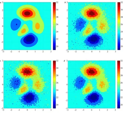
In Fig. 1, the ideal field is produced by “peaks” in MATLAB with a dimension of (100×100) (the result is shown in table 1, where MAE represents the maximum absolute error, RMSE represents the root mean square error, MAE1 represents the mean absolute error, and ME represents the mean error; the comparison of equations (5) and (6) are shown in table 2 with a dimension of (40×40)), and shown in a in Fig. 1; the background is shown in b, which is produced by superimposed random error of normal distribution on the ideal fields (same to experiments in table 2); the observation is shown in c, which is also produced by superimposed random error of normal distribution on the ideal fields (same to experiments in table 2); the analysis is shown in d, which obey equation (5).

Table 1 The result of numerical experiment with a dimension of (100×100)

MAE RMSE MAE1 ME

background field 2.7890 0.6756 0.5400 -0.0121 observation field 2.9519 0.7196 0.5756 0.0061 analysis field 1.8670 0.4927 0.3925 -0.0036

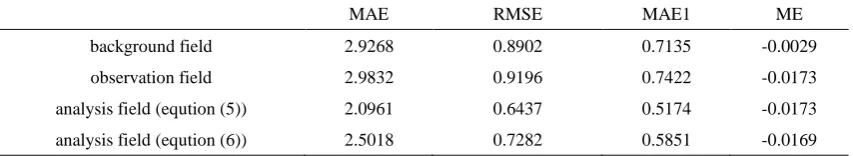
Table 2 The result of numerical experiment with a dimension of (40×40)

MAE RMSE MAE1 ME

background field 2.9268 0.8902 0.7135 -0.0029 observation field 2.9832 0.9196 0.7422 -0.0173 analysis field (eqution (5)) 2.0961 0.6437 0.5174 -0.0173 analysis field (eqution (6)) 2.5018 0.7282 0.5851 -0.0169

The result (in table 1 and 2) shows that, for the similar type of error, equation (5) is applicable. In table 1, comparing the analysis and the observation, the RMSE dropped about 0.23, the MAE1 dropped about 0.18; comparing the analysis and the background, the RMSE dropped about 0.19, the MAE1 dropped about 0.14. The analysis’ mean error is near to zero, and there is no significant abnormal value distribution in the analysis with comparing to the ideal field. In table 2, the comparison results show that the analysis obtained by equation (5) is better than the one obtained by equation (6).

The dimension of all matrixes in equation (5) is only (100×100), which can be run with personal computers. As discussion above, the dimension of background error covariance matrix is

with a dimension of (10000×10000) in equation (6), which is hard for a personal computer to allocate memory for computing.

3.

Summary

As discussed above, equation (2) is very practical, and this equation is more applicable for grid observation and can be also applied in data assimilation with conventional observation. With the calculation results in section 2.3, the assimilation effect is achieved in the numerical

experiments based on equation (2), which significantly reduces the computational magnitude. But, there are also some problems (Bannister, 2008a; Bannister, 2008b): how to construct the background error covariance matrixes B1 and B2 and observational error covariance matrixes R1

References

A. C. Lorenc. 1986. Analysis methods for numerical weather prediction. Quarterly Journal of the Royal Meteorological Society, 112: 1177–1194.

B. F. Farrell, P. J. Ioannu. 2010. State estimation using a reduced order Kalman filter. Journal of the Atmospheric Sciences, 58(23): 3666-3680.

C. Chouinard. 2003. Use of moisture sensitive satellite radiances in the Canadian Meteorological Centre Unified 3D-Var system. Proceedings of SPIE-The International Society for Optical Engineering 4895, doi: 10.1117/12/466839.

Chen Xuan, Zheng Chongwei, Zhang Weitao, Li Xin, Jin Peng. 2017. More generalized linear regression model and its meteorological application. Journal of PLA University of Science and Technology Natural Science Edition, 18(2): 144–149.

D. F. Parrish, J. D. Derber. 1992. The National Meteorological Center spectral statistical interpolation analysis system. Monthly Weather Review, 120: 1747-1763.

D. K. Sahu, S. K. Dash, S. C. Bhan. 2014. Impact of surface observations on simulation of rainfall over NCR Delhi using regional background error statistics in WRF-3DVAR model. Meteorology & Atmospheric Physics, 125 (1-2): 17-42.

P. Brousseau, L. Berre, F. Bouttier, G. Desroziers. 2015. Background-error covariances for a convective-scale data-assimilation system: AROME-France 3D-Var. 137 (655): 409-422.

R. B. Zaripov, Y. V. Martynova, V. N. Krupchatnikov, A. P. Petrov. 2016. Atmosphere data assimilation system for the Siberian region with the WRF-ARW model and three-dimensional

variational analysis WRF 3D-Var. Russian Meteorology & Hydrology, 41 (11-12): 808-815. R. N. Bannister. 2008a. A review of forecast error covariance statistics in atmospheric variational data assimilation. I: Characteristics and measurements of forecast error covariances. Quarterly Journal of the Royal Meteorological Society, 134: 1951-1970.

R. N. Bannister. 2008b. A review of forecast error covariance statistics in atmospheric variational data assimilation. II: Modelling the forecast error covariance statistics. Quarterly Journal of the Royal Meteorological Society, 134: 1971-1996.

S. E. Cohn, R. Todling. 1996. Appropriate data assimilation schemes for stable and unstable dynamics. Journal of the Meteorological Society of Japan, 74(1): 63-75.

case study over the Indian region. Meteorology & Atmospheric Physics, 112 (1-2): 63-79.

Liu Yan, Xue Jishan, Zhang Lin, Lu Huijuan. 2016. Verification and diagnostics for Data Assimilation System of Global GRAPES. Journal of Applied Meteorological Science, 27 (1): 1-15.