www.nonlin-processes-geophys.net/15/645/2008/ © Author(s) 2008. This work is distributed under the Creative Commons Attribution 3.0 License.
Nonlinear Processes
in Geophysics
Comparison between Local Ensemble Transform Kalman Filter and
PSAS in the NASA finite volume GCM – perfect model experiments
J. Liu1, E. J. Fertig2, H. Li3, E. Kalnay4, B. R. Hunt4, E. J. Kostelich5, I. Szunyogh5, and R. Todling6
1University of California, Berkeley, CA, USA 2Johns Hopkins University, Baltimore, MD, USA 3Shanghai Typhoon Institute, Shanghai, China 4University of Maryland, College Park, MD, USA 5Arizona State University, AZ, USA
6NASA-GSFC Global Modeling and Assimilation Office, Greenbelt, MD, USA
Received: 20 December 2007 – Revised: 4 April 2008 – Accepted: 10 July 2008 – Published: 5 August 2008
Abstract. This paper compares the performance of the Lo-cal Ensemble Transform Kalman Filter (LETKF) with the Physical-Space Statistical Analysis System (PSAS) under a perfect model scenario. PSAS is a 3D-Var assimilation sys-tem used operationally in the Goddard Earth Observing Sys-tem Data Assimilation SysSys-tem (GEOS-4 DAS). The compar-ison is carried out using simulated winds and geopotential height observations and the finite volume Global Circulation Model with 72 grid points zonally, 46 grid points meridion-ally and 55 vertical levels. With forty ensemble members, the LETKF obtains analyses and forecasts with significantly lower RMS errors than those from PSAS, especially over the Southern Hemisphere and oceans. This observed advantage of the LETKF over PSAS is due to the ability of the 40-member ensemble LETKF to capture flow-dependent errors and thus create a good estimate of the evolving background uncertainty. An initial decrease of the forecast errors in the Northern Hemisphere observed in the PSAS but not in the LETKF suggests that the LETKF analysis is more balanced.
1 Introduction
Three-dimensional variational data assimilation (3D-Var) was adopted for the first time in operational data assimilation at the National Centers for Environmental Prediction (NCEP) with the Spectral Statistical Interpolation (SSI) scheme in 1991 (Parrish and Derber, 1992), and has been proven to be considerably more accurate than the scheme it replaced (Op-timal Interpolation, OI). Physical-Space Statistical Analysis
Correspondence to: J. Liu
System (PSAS), a 3D-Var scheme developed at NASA1, dif-fers from other 3D-Var schemes, such as the NCEP SSI and the 3D-Var scheme of European Centre for Medium-Range Weather Forecasts (ECMWF) (Courtier et al., 1998), mainly in that it is formulated directly in physical space, rather than in spectral space (Cohn et al., 1998). It was the operational data assimilation system in the Goddard Earth Observing System Data Assimilation System (GEOS-4 DAS) (Bloom et al., 2005).
In PSAS, like in any other 3D-Var scheme, a constant sta-tistical estimate of the background error covariance is used to represent the background uncertainty. The use of a constant background error covariance makes it difficult to adjust the background (6-h forecast) toward to the true state when there are larger than average background errors that are not well represented by the background error covariance. By contrast, ensemble Kalman filter (EnKF) schemes (Evensen, 1994; Anderson, 2001; Houtekamer and Mitchell, 2001; Bishop et
1At the time of this writing, PSAS supports the following
al., 2001; Whitaker and Hamill, 2002; Tippett et al., 2003; Ott et al., 2004; Hunt et al., 2007, Kalnay et al., 2007) esti-mate a flow dependent background error covariance from a time-dependent forecast ensemble. The time changing back-ground error covariance should represent the “errors of the day” if enough ensemble members are used and the model bias is small. Recently, EnKF schemes have been shown to be able to assimilate real observations effectively. For exam-ple, Houtekamer et al. (2005) found the performance of an EnKF scheme to be comparable to the operational 3D-Var scheme when assimilating real observations into the CMC GEM grid model. With more recent changes, the perfor-mance became comparable to that of the operational 4D-Var (Houtekamer, personal communication, 2006). Whitaker et al. (2004) obtained a better mid-troposphere reanalysis from surface pressure observations with Ensemble Square Root Filter (EnSRF) (Whitaker and Hamill, 2002) than with the NCEP SSI on the GFS model at T62L28 resolution. With the same model, assimilating all operational observations except radiances, EnKF outperformed the operational SSI (Whitaker et al., 2007 and Szunyogh et al., 2008). These results show promising potential for the ensemble Kalman filter.
Unlike other ensemble Kalman filter schemes that assim-ilate observations serially (Anderson, 2001; Whitaker and Hamill, 2002; Houtekamer and Mitchell, 2001), the Local Ensemble Transform Kalman Filter (LETKF; Hunt et al., 2007) updates the local state variables of each grid point in-dependently by assimilating all observations that may affect the state at that grid point. The observations are typically selected within a small local volume centered at that grid point. The localization approach of the LETKF, which is based on the localization approach of the Local Ensemble Kalman Filter (LEKF; Ott et al., 2004), makes this assimi-lation scheme highly parallel (Szunyogh et al., 2005, 2007). Though adapted from the LEKF, the computational cost of the LETKF is significantly lower because it solves the analy-sis equations in the subspace spanned by the ensemble mem-bers without using singular value decomposition. This com-putational efficiency, simplicity of implementation (e.g., it does not require the adjoint of the observational operator and the adjoint of the model dynamics) and its accuracy make the LETKF a particularly appealing ensemble Kalman filter scheme.
While assimilation studies based on real observations pro-vide more realistic quantitative estimates of the accuracy of the proposed new schemes (e.g. Houtekamer et al., 2005; Whitaker et al., 2007; Szunyogh et al., 2008), studies based on simulated observations represent an important step toward better understanding the potential advantages and limitations of newly proposed schemes (e.g., Szunyogh et al, 2005). In the present study, we compare a once operational 3D-Var sys-tem (PSAS) with an EnKF (LETKF) by assimilating simu-lated rawinsondes on the NASA GEOS4 finite volume Gen-eral Circulation Model (fvGCM, Lin, 2004). We examine
and explain the differences in the performance of these two schemes and address the question of the ensemble size re-quired to obtain an accurate background error covariance in the LETKF.
The paper is organized as follows: The LETKF and PSAS assimilation schemes are briefly described in Sect. 2. The fvGCM is described in Sect. 3. The experimental setup is ex-plained in Sect. 4. Results comparing PSAS and the LETKF are shown in Sect. 5. Section 6 is a brief discussion of the ori-gin of the differences in the performance of the LETKF and PSAS. Section 7 illustrates the number of ensemble mem-bers required to obtain an accurate estimate of the error co-variance in the LETKF scheme. Section 8 is a summary and discussion.
2 Assimilation schemes
2.1 Physical-Space Statistical Analysis System (PSAS) PSAS (Cohn et al., 1998) solves the standard analysis equa-tions (Eqs. 1 and 2) to minimize the analysis error variance
xa=xb+K[yo−h(xb)] (1)
K=PbHT(HPbHT+R)−1 (2) Here,h(•)is a nonlinear observation operator transforming the model state variables into observation space, H is its lin-earized (Jacobian) operator and HT is the transpose (adjoint) of the Jacobian.
Unlike other 3D-Var schemes, PSAS performs most of its computations in the space of observations (Cohn et al., 1998). More specifically, PSAS applies a conjugate gradient (CG) algorithm to obtain an intermediate variablewfrom the following equation:
(HPbHT+R)w=yo−h(xb) (3) wis then substituted into Eqs. (1) and (2) to obtain the up-dated analysis state
xa=xb+PbHTw (4)
Together, Eqs. (3) and (4) are referred to as the PSAS equa-tions. In the specification of the error covariance, only the matrices HPbHT+R and PbHT are calculated and stored. These matrices depend on the observation types.
dual processor PC cluster with 2.8 GHz dual Xeon speed), we chose PSAS as the standard 3D-Var assimilation scheme with which to compare the LETKF. Also, the version of PSAS available for this study was developed to assimilate geopo-tential height observations, so we also assimilate geopoten-tial height observations in the comparison of PSAS with the LETKF.
2.2 The Local Ensemble Transform Kalman Filter
A detailed description of the LETKF is given in Hunt et al. (2007). In the following sub-sections, we briefly summa-rize the algorithm and its application on the fvGCM. For this application, we first determine the ensemble forecasts and the ensemble forecasts at observation locations (Sect. 2.2.1), then do localization around each grid point (Sect. 2.2.2). Each central grid point is updated in parallel using local in-formation (Sect. 2.2.3), and finally the analysis ensemble at every grid point are combined to obtain a global analysis for each ensemble member (Sect. 2.2.4).
2.2.1 Global ensemble forecasts
First, an ensemble of k forecasts, the ith of which is de-noted byxb(i)g , are created by integrating the fvGCM from
each analysis ensemble member valid at the previous anal-ysis time. Then, each of the forecasts is transformed into observation space by applying the observation operator. The output is denoted asyb(i)g =h(xb(i)g ), where the sub-indexg represents global vectors.
2.2.2 Localization and parallelization
A distinguishing characteristic of the LETKF is its localiza-tion scheme. Most ensemble Kalman filter techniques in-troduce covariance localization (Houtekamer and Mitchell, 2001; Hamill et al., 2001) to avoid the spurious long-distance correlations introduced by sampling with a limited number of ensemble members. The version of the LETKF used in this paper addresses this problem by cutting off a local region around each grid point (Ott et. al., 2004; Hunt et al., 2007). Only the information within the local box is used to update the center point2. There is substantial overlap between ad-jacent local regions corresponding to the neighboring grid points (Szunyogh et al., 2005). The great overlap between adjacent local boxes implies the overlap of the observation data set assimilated at the adjacent grid points, which ensures spatial continuity of the analysis (Ott et al., 2004).
2Alternatively, the localization can be based on the choice of the
observations used at each grid point (Hunt et al., 2007). This ap-proach has some advantages over the box localization adopted here, especially near the poles and for satellite observations that may de-pend on the model state in a less local way than the conventional observations.
Because the state is updated independently at each grid point, the wall-clock time needed to finish a LETKF analysis can be dramatically reduced by parallel computation. For our application, the parallel implementation is realized by separating the whole globe into a number of latitude strips based on the number of available processors. The analysis of each latitude strip is computed independently on different processors. The final analysis results do not depend on the available processors, because the assimilated observations at each local box are independent of the number of processors, and only depend on the localization scale.
Due to localization, all the vectors presented in the next subsection are reduced from global to local size. In this way, rather than having to assimilate observations serially (one af-ter the other) as in several other ensemble Kalman filaf-ter tech-niques (Tippett et al., 2003), the LETKF assimilates all rele-vant observations simultaneously (Ott et al., 2004; Szunyogh et al., 2005). Simultaneous assimilation, which allows for observation error correlations in space, is particularly impor-tant when the observation coverage is dense and correlated, such as for satellite observations. It can also assimilate obser-vations at the appropriate time when the 4-D-LETKF exten-sion is used, which allows for observation error correlations in time as well (Hunt et al., 2004; Hunt et al., 2007; Kalnay et al., 2007).
2.2.3 Local analysis
Within each latitude strip, the analysis of each grid point is performed sequentially. As described by Szunyogh et al. (2005), at each grid point, the local background vector xb(i), the corresponding local background vector in
obser-vation spaceyb(i), and the local observation vectoryoonly include the information within the local box. Different lo-calizations may be chosen for different observations, such as different localization for satellite radiances (Fertig et al., 2007). Within the local box, the background state is defined as the ensemble mean of the local forecast vectors:
xb=k−1
i=k
X
i=1
xb(i) (5)
Unlike the LEKF (Ott et. al., 2004; Szunyogh et al., 2005), the LETKF does not calculate the background error covari-ance explicitly. It calculates the background ensemble per-turbations Xbinstead. Itsith column is given byxb(i)−xb.
Following Hunt et al. (2007), the ensemble perturbations in this local box are given by
Xa=Xb(Pa)12, (6)
It is the transformation of the background ensemble pertur-bations by Pa1/2, where Pa, the analysis error covariance in the ensemble space, is given by
Pa=h(k−1)I+YbTR−1Ybi −1
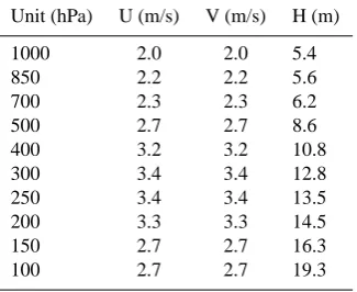
Table 1. Observation error standard deviations as a function of
ver-tical level for simulated zonal wind (U), meridional wind (V) and geopotential height (H) observations (adapted from PSAS).
Unit (hPa) U (m/s) V (m/s) H (m) 1000 2.0 2.0 5.4 850 2.2 2.2 5.6 700 2.3 2.3 6.2 500 2.7 2.7 8.6 400 3.2 3.2 10.8 300 3.4 3.4 12.8 250 3.4 3.4 13.5 200 3.3 3.3 14.5 150 2.7 2.7 16.3 100 2.7 2.7 19.3
Yb is the matrix of ensemble background perturbations in
observation space with the ith column given by yb(i)−yb,
where yb=k−1iP=k
i=1
yb(i). Because Yb is formulated using
the nonlinear observation operator, unlike 3D-Var or 4D-Var methods, the LETKF does not require either the Jacobian H of the observation operator or its adjoint HT. The ensemble mean state of LETKF is updated by the equation:
xa=xb+XbP˜aYbTR−1(yo−yb) (8) The analysis ensemble is given by adding the analysis mean to the analysis perturbations:xa(i)=Xa(i)+xa.
2.2.4 Global analysis ensemble
The local analysis described above returns the analysis en-semble for the center grid point of the local box. The analy-sis for each grid point in the latitude strip is then connected to return a single file for each strip including all ensemble members. The global analysis for each ensemble member is then extracted from these files. The global analysis ensemble is then used to initiate the ensemble forecasts discussed in Sect. 2.2.1.
3 NASA fvGCM
The dynamical core of the NASA GEOS 4 is the fvGCM developed by Lin (2004) with highly accurate numerical dis-cretization. The fvGCM solves the governing equations by employing a Lagrangian vertical coordinate. Unlike many models that forecast surface pressure, the NASA fvGCM forecasts the pressure thickness (δp)between vertical model levels and updates surface pressure (P s) as a diagnostic vari-able. The fvGCM also forecasts zonal wind (u), meridional wind (v), scaled potential temperature (θ ), and specific hu-midity (q).
The version of the fvGCM employed in our experiments has a horizontal resolution of 5◦ longitude and 4◦ latitude (72 zonal and 46 meridional grid points). The model has 55 vertical levels and includes a very high top at 0.01 hPa. We note that the horizontal resolution is coarser than that used operationally, but this allows performing a large number of experiments under our limited computational resources.
4 Simulated observations and experimental design
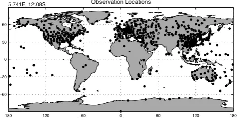
The assimilation experiments described in this study were conducted in the perfect model scenario. A nature run, rep-resenting the true state of the atmosphere, was created by running the NASA fvGCM for three months from the op-erational analysis of 16 December 2002. Simulated raw-insonde observations were obtained by converting the true model state to rawinsonde variable types, interpolating this converted true state to the real rawinsonde locations, and then adding zero-mean non-correlated Gaussian distributed noise with standard deviations same as the operationally assumed rawinsonde errors (Table 1). The observations are at the real rawinsonde observation locations shown in the left panel of Fig. 2 for 00:00 UTC, including zonal wind, meridional wind and geopotential height. A similar number of observations are available at 12:00 UTC, but far fewer are available at 06:00 UTC and 18:00 UTC (not shown).
The initial analysis cycle started at 18:00 UTC on 16 De-cember 2002 for PSAS. The initial condition used for this PSAS run was the true state from the nature run at 00:00 UTC on 15 January 2003. The LETKF analysis cycle was started on 18:00 UTC on 01 January 2003 and used the PSAS anal-ysis as the initial mean state of the ensemble. The initial ensemble members were obtained by adding normally dis-tributed noise to the mean analysis state. The standard devi-ation of the analysis ensemble perturbdevi-ations was the same as the standard deviation of the observational noise for observed variables and 0.25 K for scaled potential temperature.
The PSAS obtains analysis increments of the observed variables, and then converts these increments to update the model state variables (see Eqs. 3 and 4). The LETKF, on the other hand, directly obtains analyses for the model variables. In this study, the LETKF directly updates zonal and meridional wind, scaled potential temperature, and surface pressure. Surface pressure is not a prognostic variable, but it is used to update the related prognostic variable, pressure thickness. For simplicity and efficiency in this study, pressure thickness is updated proportionally to the surface pressure increment for each ensemble member. Specifically, the analysis increment of the pressure thickness at levelkfor theith ensemble member is given by
1δpa(i)k
δpb(i)k
=1P s a(i) k
P sb(i)k ,
ï180 ï120 ï60 0 60 120 180 ï60 ï30 0 30 60 Observation Locations 5.741E, 12.08S
Fig. 1. Left panel: real rawinsonde observation locations (black
dots) at 00:00 UTC. Right panel: relative distribution of observa-tional coverage at different pressure levels.
where1indicates the analysis increment of the correspond-ing variable. Furthermore, neither the LETKF nor the PSAS updates specific humidity in this study to avoid the complexi-ties of assimilating humidity observations (Dee and DaSilva, 2003). We have a separate study examining the impact of assimilating humidity with the LETKF (Liu, 2007).
Sampling errors and the effects of nonlinearities in the evolution of the estimation errors can lead to an underesti-mation of the background error covariance and to filter di-vergence (e.g., Whitaker and Hamill, 2002). To compensate for this problem, a multiplicative variance inflation scheme (Anderson and Anderson, 1999) is employed in the LETKF. In practice, we achieve this as in Hunt et al. (2007) by modi-fying Eq. (7):
˜ Pa=
(k−1)
1+ρ I+Y
bTR−1Yb
−1
, (10)
whereρis a positive number, and(1+ρ)is the inflation fac-tor. The main difference between the approach of Anderson and Anderson (1999) and that of Hunt et al. (2007) is that while the former scheme inflates the ensemble background perturbations, Eq. (10) inflates the analysis perturbations. These two approaches would be equivalent if the evolution of the ensemble perturbations is strictly linear. The inflation factor,ρ, is tuned to change with vertical levels, latitudes, and time (see Tables 2 and 3). At the lower levels the inflation factor was kept constant throughout the assimilation cycle (8% over the entire globe). For the levels above 100 hPa, the inflation factor was larger during spin-up time. We found ex-perimentally that such large inflation above 100 hPa (Table 2) is useful for the first few analysis steps before the analysis er-ror settles at a stationary level. Once the system settles, the inflation is decreased from 8% at 100 hPa to about 5% over the polar region (Table 3). To avoid changing inflation factor abruptly either in vertical or meridional direction, we linearly change these inflation factors. In the local boxes where there is no observation, we do not inflate the background, though later studies have found that the analysis improves slightly
Table 2. Inflation factors as a function of vertical levels and latitude
bands for spin-up.
Unit: hPa 90◦S–14◦S 10◦S–6◦N 10◦N–26◦N 30◦N–90◦N
976.7–118.2 1.08 1.08 1.08 1.08
100.5 1.09 1.09 1.09 1.09
85.4 1.10 1.10 1.10 1.10
72.6 1.20 1.20 1.20 1.20
61.5 1.25 1.30 1.30 1.30
52.0 1.35 1.40 1.40 1.40
43.9 1.35 1.50 1.50 1.50
37.0 1.35 1.50 1.60 1.60
31.1 1.35 1.50 1.70 1.70
26.0 1.35 1.50 1.70 1.80
21.8 1.35 1.50 1.70 1.90
18.1–0.015 1.35 1.50 1.70 2.00
by also inflating the background in these regions (Szunyogh et al., 2007).
The dimensions of the local box were varied spatially to account for inhomogeneous observation coverage and the change of physical distance between grid points with lati-tudes. The width of the box was increased in the Southern Hemisphere (SH), where observations are sparse. To account for the convergence of the meridians toward the poles, the number of grid points in zonal direction included in the local box was also increased with latitude in both Hemispheres. For example, the horizontal local patch was 7 grid points by 7 grid points in the mid-latitudes in the Northern Hemisphere (NH), while it was increased to 15 grid points by 7 grid points near the poles. The vertical dimension of the local boxes contained 3 vertical levels, except at the top and the bottom model levels where they contained 1 level. In the newer con-figuration of the LETKF (Hunt et al., 2007), the localization scale only depends on the actual physical distance, requiring less tuning.
We tuned the variance of background error covariance used by PSAS to account for the fact that it was originally tuned using real observations and found that the results were not very sensitive to this amplitude. Since we did not tune the correlation structure, the PSAS results presented below may not be optimal. So the advantage of the LETKF over PSAS may not be as large as the results shown here.
5 Relative performance of the LETKF and the PSAS
Table 3. Inflation factors as a function of vertical levels and latitude bands for stable state.
Unit: hPa 90◦S–62◦S 90◦S–14◦S 10◦S–6◦N 10◦N–50◦N 54◦N–66◦N 70◦N–90◦N 976.7–18.2 1.08 1.08 1.08 1.08 1.08 1.08 100.5 1.09 1.09 1.09 1.09 1.09 1.09 85.4 1.10 1.10 1.10 1.10 1.10 1.10 72.6 1.09 1.15 1.20 1.20 1.20 1.10 61.5 1.08 1.20 1.30 1.30 1.30 1.10 52.0 1.07 1.20 1.30 1.40 1.30 1.10 43.9 1.06 1.20 1.30 1.50 1.30 1.10 37.0 1.05 1.20 1.30 1.60 1.30 1.10 31.1 1.05 1.20 1.30 1.60 1.30 1.10 26.0 1.05 1.20 1.30 1.60 1.30 1.10 21.8 1.05 1.20 1.30 1.60 1.30 1.10 18.1–0.015 1.05 1.20 1.30 1.60 1.30 1.10
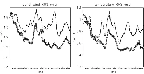
Fig. 2. 500 hPa global average analysis RMS error (y-axis) as function of time (x-axis) for zonal wind (left panel) and temperature (right
panel). Dashed line: PSAS; solid line with open circles: the LETKF.
LETKF over PSAS (RMS error difference between LETKF and PSAS normalized by the PSAS RMS error). Negative values indicate that LETKF is better than PSAS. For the fore-casts, we compare the 5-day forecast RMS error from these two schemes in different areas, as well as the representation and the impact of gravity waves on the forecast.
5.1 Time series of analysis RMS error
The RMS error time series start from 00:00 UTC, 2 Jan-uary 2003, when PSAS analysis has already settled, and the LETKF analysis cycle begins. As shown in Fig. 2, after a few days the LETKF analysis (solid line with open circles) has
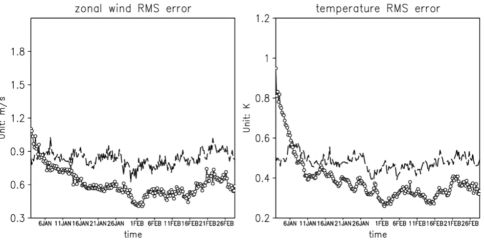
Fig. 3. Same as Fig. 2, except for the analysis RMS error averaged over the Northern Hemisphere (22◦N–90◦N).
error for both schemes. Because the density of rawinsonde network is highest in the NH (Fig. 1), the background quickly adjusts to the observations there. Therefore, most of the fluc-tuations of the errors appear in the regions with low obser-vation density, like the extratropical SH (22◦S–90◦S) and oceans.
5.2 Vertical and latitudinal structure of the analysis error Figures 2 and 3 show that the LETKF analysis RMS errors at 500 hPa are smaller than those of PSAS. We further compare the RMS errors at all vertical levels below 100 hPa, shown in Fig. 4. It shows that the LETKF analysis RMS errors are smaller at all model levels for both zonal wind (left panel) and temperature (right panel). The RMS error is significantly smaller than the observational error (Table 1) for both PSAS (dashed line in Fig. 4) and the LETKF (solid line with open circles in Fig. 4). The percentage improvement relative to PSAS is about 40% for zonal wind and 30% for temperature (not shown). The improvement is larger at the lower levels than at the higher levels. For the levels above 100 hPa (not shown), the RMS errors of both the LETKF and PSAS in-crease sharply, with the LETKF inin-creases faster. At around 80 hPa, the accuracy of PSAS surpasses the LETKF. We need to further investigate the reason for the better performance of PSAS above 100 hPa.
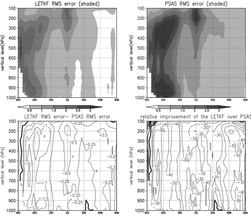
Figure 5 compares zonally and temporally averaged anal-ysis RMS errors from PSAS and LETKF. In the NH, where both schemes provide more accurate analysis, the LETKF has smaller errors than PSAS (bottom left panel in Fig. 5).
The zonal wind analysis RMS error of the LETKF is only between 0.25 m/s and 0.5 m/s at high latitudes (top left panel in Fig. 5), which is about 15% to 25% of the observation error. In most of the tropics and SH, where the RMS er-rors are larger, the difference between the RMS error of the LETKF and PSAS is also larger (bottom left panel in Fig. 5), especially over SH. Although the RMS error over the trop-ics is large for both schemes, the error reduction of LETKF compared with PSAS is between−30% and−40% in this re-gion (bottom right panel in Fig. 5). The percentage improve-ment is between−40% and−50% through the whole ver-tical column over the mid-latitudes in the SH (bottom right panel in Fig. 5). However, the percentage improvement be-comes smaller beyond 70◦S toward the South Pole, where the LETKF analysis becomes slightly worse than PSAS. The assimilation near the poles was a challenge for the present lo-cal box formulation of LETKF (see footnote in Sect. 2.2.2). 5.3 Comparison of forecast errors
Fig. 4. Time mean (averaged over February) of the analysis RMS error averaged over the globe as function of vertical levels for zonal wind
(top left panel) and temperature (top right panel). Dashed line: PSAS; solid line with open circles: the LETKF.
errors disperse, and the growing modes start dominating the error, do we expect to observe exponential growth. There-fore, the error growth observed in different areas provides an indication of the type of errors and the relative balance of the analysis.
As expected, the forecast RMS errors from the LETKF analysis are smaller than that from PSAS analysis (dashed line) during a 5-day forecast period over all the regions (Fig. 6). However, different regions show different charac-teristics of error growth. In the NH (top left panel in Fig. 6), PSAS errors initially decay, and start growing after about a day, indicating that the PSAS analyses are not well balanced. With the same set of observations, the LETKF starts with smaller errors, but they grow faster. In the SH (top right panel in Fig. 6), the errors of PSAS start growing immediately af-ter the analysis, suggesting that the PSAS analysis is more balanced in the SH than in the NH. This is not surprising, since the number of observations in the SH is much smaller than in the NH, and it is the assimilation of observations that cause the PSAS analysis to lose its balance (The assimilation of observations takes place within the subspace spanned by the PSAS background error covariance). The forecast RMS errors of LETKF grow at a smaller rate than PSAS after an initial slight decrease during the first 6 h. The initial error decrease is presumably associated with the convective im-balance in the SH summer (Harlim et al., 2005). In the trop-ics (22◦S–22◦N, bottom left panel in Fig. 6), the forecast RMS errors of PSAS are almost constant for a couple of days, and then increase linearly. For the LETKF the
fore-cast RMS errors start smaller than PSAS and grow linearly with time at about the same rate as PSAS. This characteris-tic linear growth of errors in the tropics was also observed in Kuhl et al. (2007) in simulations with the NCEP Global Forecasting System (GFS). Unlike extratropical error growth dominated by slow baroclinic waves, tropical errors are dom-inated by convection, which saturate almost immediately at small scales and slowly propagate to larger scales even in a perfect model scenario (Kalnay, 2003; Harlim et al., 2005). 5.4 Accuracy in representing gravity waves
Maintaining atmospheric balance is particularly important during data assimilation. Imbalance in the atmospheric anal-ysis will result in the excitation of spurious gravity waves, which eventually will ruin the accuracy of the data assimila-tion system. Gravity waves are generally not observed with significant amplitudes, except for the diurnal and semidiur-nal tides. So the goal during data assimilation is to retain the gravity waves present in reality, but to avoid exciting spuri-ous gravity waves.
Fig. 5. The contours in the two figures in top panel indicate the time average (over February) of the true zonal wind field, and the shades
indicate the zonal average of the time mean zonal wind analysis RMS error of the LETKF (top left panel) and PSAS (top right panel). Bottom left panel is the analysis RMS error difference between the LETKF and PSAS, and the bottom right panel is the relative improvement of the LETKF over PSAS. The thicker line in both figures in the bottom panel is zero line.
begins. In the current implementation of both the PSAS and the LETKF, there is no such extra constraint. The ensem-ble analyses in the LETKF minimize the introduction of spu-rious gravity waves by computing the analyses as a linear combination of the ensemble forecasts, which are generally well balanced. Fast gravity waves remain in the analysis field only if they are in the background. Although the use of local boxes in the LETKF could lead to imbalances, the large overlap between different local boxes (as discussed in Sect. 2) in the LETKF is apparently able to minimize the excitement of gravity waves by assimilating similar informa-tion in neighboring regions. We compare the relative ability
Fig. 6. 500 hPa zonal wind forecast RMS error (m/s), averaged over February, as a function of the leading time in different regions. Top
left panel: Northern Hemisphere (22◦N–90◦N); Top right panel: Southern Hemisphere (22◦S–90◦S); Bottom left panel: Tropics (22◦S– 22◦N); Bottom right panel: the globe. Dashed line: PSAS; solid line with open circles: the LETKF.
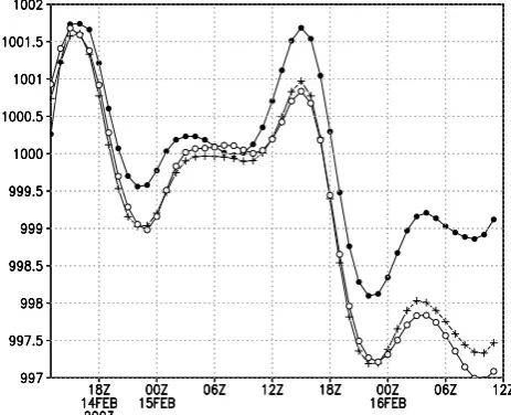
larger than that of LETKF. The gravity wave that appears in the truth has both diurnal and semi-diurnal components, especially around 14 February. This structure is more appar-ent in the 2-day forecasts starting on 12:00 UTC 14 February plotted every hour (bottom panel in Fig. 7). The forecasted surface pressure shows the diurnal and semidiurnal modes in the truth (crosses), PSAS (full circles), and LETKF (open cir-cles) forecasts. Although both forecasts capture the diurnal and semidiurnal tides, we observe that the initial conditions from the LETKF lead to a more balanced and accurate fore-cast. We have to note that the observation coverage in the
Fig. 7. Upper left panel: the “true” analyzed divergence field every 6 h at 32◦N, 93◦W on 700 hPa (where there is a rawinsonde observation). Upper right panel: the divergence error for the LETKF (open circles) and PSAS (closed circles). The bottom panel: 2-day surface pressure forecast from 12:00 Z, 14 February at 32◦N, 93◦W (crosses show the true pressure, open circles are the LETKF forecast, and full circles are the PSAS forecast). The output interval is every hour.
6 The relationship between analysis increments and background error
The analysis increments (the difference between analysis state and background state) reflect the correction made to the background with the observed information. They are deter-mined by the background error covariance, observation error, and observation innovation (the difference between observa-tion and the background mean state in the observaobserva-tion space), as shown in Eq. (1) for PSAS and Eq. (8) for LETKF. The background error is the difference between background state and the truth, so that the optimal analysis increments should be equal and opposite sign of the background errors. We analyze reasons for the difference in the performance of the LETKF and PSAS by examining the relationship between
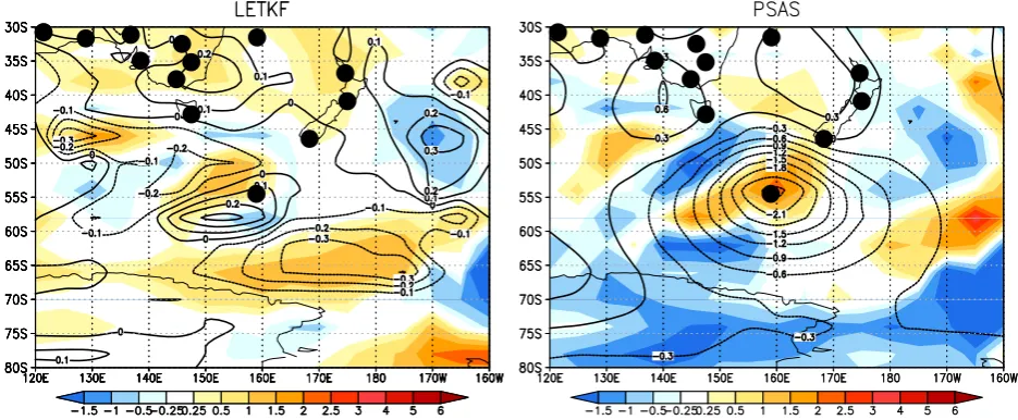
Fig. 8. 500 hPa temperature analysis increments (contours) and background error (shaded) for the LETKF (left panel) and PSAS (right panel)
at 12:00 Z, 12 February. The dots represent the rawinsonde observation locations.
without observations. Since the LETKF and PSAS assimi-late the same observation and use the same observation error statistics, this different characteristic of analysis increments is mainly due to different background error statistics. The background error covariance estimated from the ensemble is able to extrapolate observation information to data sparse re-gions by accurately reflecting the shape of the errors of the day, so the analysis increments have the similar shape with the background error. Because PSAS has a constant isotropic background error covariance, it cannot estimate abrupt error changes in the shape and amplitude of background error. As a result, the structure of the PSAS temperature increments is significantly different from that of the background error (right panel in Fig. 8). In PSAS, the large analysis incre-ments are observed around the observation locations, not in regions with large background error.
7 Estimation of the sufficiency of the number of ensem-ble members used in the LETKF
One measure of the sufficiency of the number of ensemble members is the consistency between the background uncer-tainty estimated from the background ensemble forecasts and the true background error. Ideally, with perfect model exper-iments and with enough ensemble members, the estimated background uncertainty should be same with the actual back-ground error. When there are too few ensemble members, the background uncertainties estimated from the ensemble would be far from the actual background error.
Ensemble spread is used to represent the background un-certainty estimated from ensemble forecasts, which is the di-agonal value of the background error covariance. We exam-ine the ability of 40 ensemble members to adequately
repre-sent the true uncertainty by comparing the ensemble spread to the actual ensemble mean error. Both quantities are aver-aged over the second month of the assimilation cycle. The time average of the ensemble spread is calculated as follows:
S=
"
1 T
t=T
X
t=1
1 k−1
i=k
X
i=1
(xbi−xb)2
#12
, (11)
HereSrepresents the time-averaged ensemble spread of any dynamical variable at any grid point, wherexibis the it h back-ground ensemble member and xb is the background mean
state at that grid point. The error of the ensemble mean is measured by the distance between the background ensemble mean and the true state:
V=
"
1 T
i=T
X
i=1
(xb−xt)2
#12
, (12)
wherext is the true state at that grid point. If the data assim-ilation is optimal, and there are enough ensemble members to estimate the background error covariance, the background ensemble spread should be same as the error of the ensemble mean.
Fig. 9. Time average ensemble spread of zonal wind (averaged over
February, contour; Unit: m/s) and the ensemble mean error (shades; Unit: m/s) at 500 hPa.
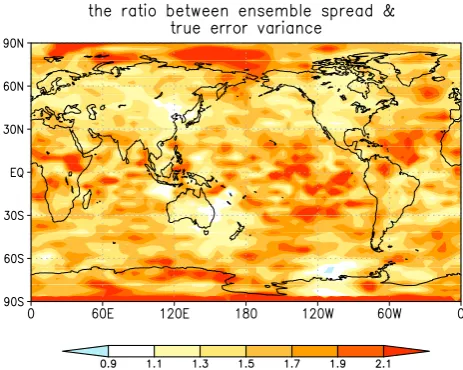
that larger inflation factors are required in the data dense re-gion to keep a reasonable ensemble spread. In data sparse regions such as the tropics, the ratio of ensemble spread to variance is about 1.5–2 (Fig. 10), which suggests that the ensemble spread overestimates the background uncertainty, causing the analysis to give more weight to the observations than it should. Further tuning the inflation factor based on the observation coverage may improve the assimilation accu-racy, since inflation should be different over data dense and data sparse regions.
Our results suggest that 40 ensemble members are enough to adequately capture the background uncertainty under the perfect model scenario with the limited observing system used and model resolution. We recognize that the resolution of the model used for this study is much coarser than that of operational models. Accordingly, more than 40 ensemble members may be required to estimate the background error covariance for operational models. However, the number of ensemble members required is not unlimited. Miyoshi and Yamane (2007) show that 80 ensemble members are enough to get good performance with T159/L48 (corresponding to a grid of 480×240×48) AGCM and much denser observa-tions.
8 Summary and discussion
In this study we compare the performance of the LETKF with the NASA PSAS analysis system (GEOS-4 data assim-ilation system) by assimilating simulated rawinsonde obser-vations on a finite volume GCM with horizontal resolution of 4◦by 5◦and 55 vertical levels. With 40 ensemble mem-bers, the LETKF analyses show significantly less RMS er-ror than the PSAS analyses. The largest improvement of the
Fig. 10. The ratio of time average ensemble spread and ensemble
mean error of zonal wind at 500 hPa.
LETKF over PSAS is found in regions with sparse observa-tions, particularly in the Southern Hemisphere. This result is consistent with Whitaker et al. (2004, 2007) and Szunyogh et al. (2007) finding that ensemble Kalman filters have the most advantage over a 3D-Var in data sparse regions. The 5-day forecasts maintain this advantage. The forecast errors starting from the PSAS analysis in the NH slightly decrease in the first few hours before they start growing with time, indicating the presence of analysis imbalance that disperses as gravity waves during the initial geostrophic adjustment. By contrast, the initially smaller analysis error in the LETKF analysis grows exponentially, indicating better balance in the initial conditions.
We believe that the large improvement of the LETKF over the PSAS is due to the fact that the background error covari-ance used in the LETKF varies realistically with space and time, but the constant background error covariance used in the PSAS cannot reflect abrupt error changes in the back-ground. As a result, the analysis increments structure are more similar (with opposite sign) to the background errors in the LETKF, whereas in PSAS the analysis corrections are more isotropic, and tend to be centered at observation loca-tions. The accuracy of the background error covariance esti-mation is crucial to the performance of the LETKF scheme, and is related to the number of ensemble members. The agreement between ensemble spread and ensemble mean er-ror suggests that forty ensemble members used in the LETKF are sufficient to capture most of the uncertainty in the global fvGCM forecast. Nevertheless, more ensemble members may be required in a higher resolution model.
scheme. In this version of the LETKF, the localization is based on the number of grid points in each local box around the center point. Only those observations within a local box are used to update the center grid point. Alternatively, the lo-calization can be based on choosing the observations within a distance to update the center grid point, rather than using a local box (Hunt et al., 2007).
Although in this study we compared the LETKF with the 3D-Var analysis scheme used in the NASA GEOS-4 opera-tional system, some caveats about the results should be men-tioned. Our experiments are based on a perfect model sce-nario, in which we have avoided additional challenges asso-ciated with the presence of unknown observation and model errors. Also, the observational network only includes rawin-sondes, which is much sparser than the operational observa-tion network. Previous research shows that EnKF has more advantage in data sparse region (Whitaker et al., 2004) so that the advantages of the LETKF should be smaller for currently available operational observations than our results indicate. In addition, the error statistics of PSAS has not been well tuned, and the model resolution used is lower than that cur-rently used in operations. Therefore our very encouraging results could be interpreted as an upper bound for the poten-tial operational advantage of EnKF over 3D-Var. GEOS-4 has been replaced by the GEOS-5 system, which in the fu-ture should be also compared with the LETKF.
Acknowledgements. This work is part of the research towards
the fulfillment of the doctorate requirement of the three leading authors, who have contributed equally. This research was partially supported by NSF ATM9328402, NASA NNG04GK29G and NNG04GK78A. We are grateful to Dirceu Herdies, Arlindo DaSilva and Shian-Jiann Lin for very helpful discussions. Two anonymous reviewers provided us with very constructive and detailed comments that helped clarify several aspects of this study. Edited by: Z. Toth
Reviewed by: two anonymous referees
References
Anderson, J. L.: An ensemble adjustment Kalman filter for data assimilation, Mon. Weather Rev., 129, 2884–2903, 2001. Anderson, J. L. and Anderson, S. L.: A Monte Carlo
implementa-tion of the nonlinear filtering problem to produce ensemble as-similations and forecasts, Mon. Weather Rev., 127, 2741–2758, 1999.
Bishop, C. H., Etherton, B., and Majumdar, S. J.: Adaptive sam-pling with the ensemble transform Kalman filter – Part I: Theo-retical aspects, Mon. Weather Rev., 129, 420–436, 2001. Bloom, S. C., Takacs, L. L., DaSilva, A. M., and Ledvina, D.: Data
assimilation using incremental analysis updates, Mon. Weather Rev., 124, 1256–1271,1996.
Bloom, S. C., DaSilva, A., Dee, D., et al.: Documentation and val-idation of the Goddard Earth Observing System (GOES) Data Assimilation System – Version 4, Technical report series on
global modeling and data assimilation, 26, available at: http: //gmao.gsfc.nasa.gov/systems/geos4/Bloom.pdf, 2005.
Cohn, S. E., DaSilva, A. M., Guo, J., Sienkiewicz, M., and Lamich, D.: Assessing the Effects of Data Selection with the DAO Physical-Space Statistical Analysis System, Mon. Weather Rev., 126, 2913–2926, 1998.
Courtier, P., Anderson, E., Heckley, W., Pailleux, J., Vasiljevic, D., Hamrud, M., Hollingsworth, A., Rabier, F., and Fisher, M.: The ECMWF implementation of three-dimensional variational assimilation (3D-Var) – I: Formulation, Q. J. Roy. Meteor. Soc., 124, 1783–1807, 1998.
Daley, R.: Atmospheric data analysis, Cambridge University Press, Cambridge, UK, 471 pp., 1991.
Dee, D. P. and DaSilva, A. M.: The choice of variable for atmo-spheric moisture analysis, Mon. Weather Rev., 131, 155–171, 2003.
Evensen, G.: Sequential data assimilation with a nonlinear quasi-geostrophic model using Monte Carlo methods to forecast error statistics, J. Geophys. Res., 99(C5), 10 143–10 162, 1994. Fertig, E. J., Hunt, B. R., Ott, E., and Szunyogh, I.:
Assimilat-ing nonlocal observations with a Local Ensemble Kalman Filter, Tellus A, 59, 719–730, 2007.
Hamill, T. M., Whitaker, J. S., and Snyder, C.: Distance-dependent filtering of background error covariance estimates in an ensemble Kalman filter, Mon. Weather Rev., 129, 2776–2790, 2001. Harlim, J., Hunt, B. R., Kalnay, E., and Yorke, J. A.:
Convex error growth, Phys. Rev. Lett., 94, 228501, doi:10.1103/PhysRevLett.94.228501, 2005.
Houtekamer, P. L. and Mitchell, H. L.: A sequential Ensemble Kalman Filter for atmospheric data assimilation, Mon. Weather Rev., 129, 123–137, 2001.
Houtekamer, P. L, Mitchell, H. L., Pellerin, G., Buehner, M., Char-ron, M., Spacek, L., and Hansen, B.: Atmospheric data assimila-tion with the ensemble Kalman filter: Results with real observa-tions, Mon. Weather Rev., 133, 604–620, 2005.
Hunt, B. R., Kalnay, E., Kostelich, E. J., Ott, E., Patil, D. J., Sauer, T., Szunyogh, I., Yorke, J. A., and Zimin, A. V.: Four-dimensional ensemble Kalman filtering, Tellus A, 56(4), 273– 277, 2004.
Hunt, B. R., Kostelich, E. J., and Szunyogh, I.: Efficient Data As-similation for Spatiotemporal Chaos: a Local Ensemble Trans-form Kalman Filter, Physica D, 230, 112–126, 2007.
Kalnay, E.: Atmospheric modeling, data assimilation and pre-dictability, Cambridge Univ. Press, Cambridge, UK, 341 pp., 2003.
Kalnay, E., Li, H., Miyoshi, T., Yang, S.-C., and Ballabrera-Poy, J. B.: 4D-Var or ensemble Kalman filter?, Tellus A, 59, 758–773, 2007.
Kuhl, D. D., Szunyogh, I., Kostelich, E. J., Patil, D. J., Gyarmati, G., Oczkowski, M., Hunt, B. R., Kalnay, E., Ott, E., and Yorke, J. A.: Assessing predictability with a Local Ensemble Kalman Filter, J. Atmos. Sci., 64, 1116–1140, 2007.
Lin, S. J.: A “Vertically Lagrangian” Finite-Volume Dynamical Core for Global Models, Mon. Weather Rev., 132, 2293–2307, 2004.
using a digitial filter, Mon. Weather Rev., 120, 1019–1034, 1992. Miyoshi, T. and Yamane, S.: Local Ensemble Transform Kalman Filtering with an AGCM at a T159/L48 resolution, Mon. Weather Rev., 135, 3841–3861, 2007.
Ott, E., Hunt, B. R., Szunyogh, I., Zimin, A. V., Kostelich, E. J., Corazza, M., Kalnay, E., Patil, D. J., and Yorke, J. A.: A Lo-cal Ensemble Kalman Filter for Atmospheric Data Assimilation, Tellus A, 56, 415–428, 2004.
Parrish, D. F. and Derber, J. C.: The National Meteorological Center’s spectral statistical-interpolation analysis system, Mon. Weather Rev., 120, 1747–1763, 1992.
Szunyogh, I., Kostelich, E. J., Gyarmati, G., Kalnay, E., Hunt, B. R., Ott, E., Satterfield, E., and Yorke, J. A.: A Local Ensemble Transform Kalman filter data assimilation for the NCEP global model, Tellus A, 60, 113–130, 2008.
Szunyogh, I., Kostelich, E. J., Gyarmati, G., Patil, D. J., Hunt, B. R., Kalnay, E., Ott, E., and Yorke, J. A.: Assessing a Local Ensem-ble Kalman Filter: Perfect Model Experiments with the NCEP Global Model, Tellus A, 57, 528–545, 2005.
Tippett, M. K., Anderson, J. L., Bishop, C. H., Hamill, T. M., and Whitaker, J. S.: Ensemble square root filters, Mon. Weather Rev., 131, 1485–1490, 2003.
Toth, Z. and Kalnay, E.: Ensemble Forecasting at NCEP and the Breeding Method, Mon. Weather Rev., 125, 3297–3319, 1997. Whitaker, J. S. and Hamill, T. M.: Ensemble data assimilation
with-out perturbed observations, Mon. Weather Rev., 130, 1913–1924, 2002.
Whitaker, J. S., Compo, G. P., Wei, X. and Hamill, T. M.: Reanaly-sis without radiosondes using ensemble data assimilation, Mon. Weather Rev., 132, 1190–1200, 2004.