www.atmos-meas-tech.net/10/351/2017/ doi:10.5194/amt-10-351-2017
© Author(s) 2017. CC Attribution 3.0 License.
Global clear-sky surface skin temperature from multiple
satellites using a single-channel algorithm with angular
anisotropy corrections
Benjamin R. Scarino1, Patrick Minnis2, Thad Chee1, Kristopher M. Bedka2, Christopher R. Yost1, and Rabindra Palikonda1
1Science Systems and Applications, Inc., 1 Enterprise Parkway, Suite 200, Hampton, VA 23666, USA 2NASA Langley Research Center, 21 Langley Blvd MS 420, Hampton, VA 23681-2199, USA
Correspondence to:Benjamin R. Scarino ([email protected])
Received: 10 March 2016 – Published in Atmos. Meas. Tech. Discuss.: 5 April 2016 Revised: 22 November 2016 – Accepted: 19 December 2016 – Published: 27 January 2017
Abstract. Surface skin temperature (Ts) is an important parameter for characterizing the energy exchange at the ground/water–atmosphere interface. The Satellite ClOud and Radiation Property retrieval System (SatCORPS) employs a single-channel thermal-infrared (TIR) method to retrieveTs over clear-sky land and ocean surfaces from data taken by geostationary Earth orbit (GEO) and low Earth orbit (LEO) satellite imagers. GEO satellites can provide somewhat con-tinuous estimates of Ts over the diurnal cycle in non-polar regions, while polarTsretrievals from LEO imagers, such as the Advanced Very High Resolution Radiometer (AVHRR), can complement the GEO measurements. The combined global coverage of remotely sensed Ts, along with accom-panying cloud and surface radiation parameters, produced in near-realtime and from historical satellite data, should be beneficial for both weather and climate applications. For ex-ample, near-realtime hourly Ts observations can be assimi-lated in high-temporal-resolution numerical weather predic-tion models and historical observapredic-tions can be used for val-idation or assimilation of climate models. Key drawbacks to the utility of TIR-derived Ts data include the limitation to clear-sky conditions, the reliance on a particular set of analy-ses/reanalyses necessary for atmospheric corrections, and the dependence on viewing and illumination angles. Therefore, Ts validation with established references is essential, as is proper evaluation ofTssensitivity to atmospheric correction source.
This article presents improvements on the NASA Langley GEO satellite and AVHRR TIR-basedTs product that is
de-rived using a single-channel technique. The resulting clear-sky skin temperature values are validated with surface ref-erences and independent satellite products. Furthermore, an empirically adjusted theoretical model of satellite land sur-face temperature (LST) angular anisotropy is tested to im-prove satellite LST retrievals. Application of the anisotropic correction yields reduced mean bias and improved preci-sion of GOES-13 LST relative to independent Moderate-resolution Imaging Spectroradiometer (MYD11_L2) LST and Atmospheric Radiation Measurement Program ground station measurements. It also significantly reduces inter-satellite differences between LSTs retrieved simultaneously from two different imagers. The implementation of these universal corrections into the SatCORPS product can yield significant improvement in near-global-scale, near-realtime, satellite-based LST measurements. The immediate availabil-ity and broad coverage of these skin temperature observa-tions should prove valuable to modelers and climate re-searchers looking for improved forecasts and better under-standing of the global climate model.
1 Introduction
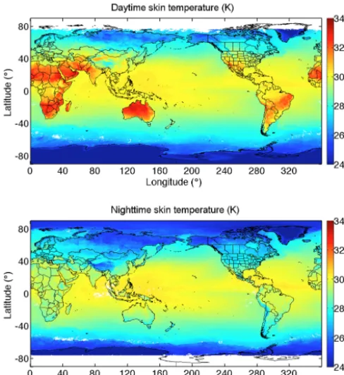
en-Figure 1.Mean merged, clear-sky surface skin temperature values from GOES-East, GOES-West, Meteosat-9, MTSAT-2, and INSAT-3D, October 2015.
ergy balance and top-of-atmosphere (TOA) radiative budget calculations rely on the accuracy of these surface parame-ters (Bodas-Salcedo et al., 2008). In addition to surface flux analyses,Tsretrievals are used to minimize model prediction uncertainty by updating model state values with observations at regular time steps – an important consideration for climate and numerical weather prediction (NWP) models (Garand, 2003; Tsuang et al., 2008; Reichle et al., 2010; Ghent et al., 2010; Guillevic et al., 2012; Draper et al., 2015). The mod-eling community could benefit significantly from the provi-sion of frequent, spatially contiguous, global land and ocean Ts data (Rodell et al., 2004; Bosilovich et al., 2007). Many other uses ofTsas well as the status and future ofTsretrievals are summarized by Li et al. (2013). It is clear that the need is growing for higher accuracy, global coverage, and greater temporal and spatial resolution ofTs retrievals from satellite imager data.
Satellite-basedTsretrieval, validation, and modeling stud-ies originate from a variety of sources, e.g., the National En-vironmental Satellite, Data, and Information Service (NES-DIS) or the National Oceanic and Atmospheric Adminis-tration (NOAA) via the Advanced Very High Resolution Radiometer (AVHRR) series and the Geostationary Opera-tional Environmental Satellite (GOES) sensors (Prata, 1993, 1994; Coll and Caselles, 1997; Sobrino and Raissouni, 2000; Kerr et al., 2004; Sobrino et al., 2004; Yu et al., 2009, 2012a, b; Sun et al., 2012). Specifically, using two dif-ferent single-channel land surface temperature (LST) algo-rithms, Heidinger et al. (2013) and Minnis et al. (2016)
found good agreement with the NOAA ESRL Surface Ra-diation (SURFRAD) network in verification studies using LST retrievals from GOES and AVHRR alone, respectively. Furthermore, near-realtime (NRT) LST is produced opera-tionally from Meteosat Spinning Enhanced Visible and In-frared Imager (SEVIRI) data, which offer continuous cover-age of Europe and Africa, and served as the focus of sev-eral LST validation studies (Sobrino and Romaguera, 2004; DaCamara, 2006; Kabsch et al., 2008; Trigo et al., 2008; Göttsche et al., 2013). Retrievals using radiances from the Moderate Resolution Imaging Spectroradiometer (MODIS) have been both the target and standard for a number of LST verification studies (Wan et al., 2002, 2004, 2008; Coll et al., 2009; Jiménez et al., 2012). Duan et al. (2014) used four daily observations from Terra and Aqua MODIS to capture the diurnal cycle of LST, which is critical for full character-ization of the climate system. Wang et al. (2014) conducted a three-wayTscomparison using MODIS, in situ ground ob-servations, and model simulations. They note the high impor-tance of accurate cloud-clearing and the inherit difficulties of resolution scaling when comparisons are conducted between satellite data and point references – conclusions supported in a similar MODIS daytime LST verification study conducted by Williamson et al. (2013).
Me-Figure 2. Average surface skin temperature from NOAA-19 AVHRR, October 2013.
teosat Second Generation (MSG; 9 or Meteosat-10), MTSAT-2 (recently replaced by Himawari-8), and the Indian Space Research Organization INSAT-3D provides high-temporal-resolution (1 h nominal) quasi-globalTs data produced in NRT, with a shared single-channel retrieval al-gorithm (e.g., Fig. 1). The methodology (Sect. 3) is flexible and easily transportable to other GEO and LEO imagers, in-cluding the current AVHRR instruments on the NOAA and EUMETSAT MetOp platforms. AVHRRTsretrievals supple-ment the GEO data and fill in missing measuresupple-ments over polar regions (e.g., Fig. 2). This same method is being ap-plied to historic and current imager datasets, particularly as part of the Satellite ClOud and Radiative Property retrieval System (SatCORPS) analyses of AVHRR data for provision of a NOAA Climate Data Record (Minnis et al., 2016), and for MODIS, GEO, and Suomi National Polar-orbiting Part-nership (S-NPP) Visible Infrared Imaging Radiometer Suite data as part of the Clouds and Earth’s Radiant Energy System (CERES) project (e.g., Minnis et al., 2010).
This article highlights recent improvements made to the SatCORPS NRT satelliteTs product (Scarino et al., 2013), via comparisons of GOES and AVHRRTsretrievals with es-tablished sea surface temperature (SST) and LST reference datasets. The influence of NWP source on retrievedTs val-ues is also examined. The main improvements over the ear-lier version are enhanced pixel-level resolution output and hourly GEO retrieval time steps. The SatCORPSTsretrieved
from GOES and AVHRR data is evaluated by comparing with reference datasets based on in situ and satellite mea-surements. Section 2 provides an overview of these product and reference datasets, as well descriptions of ancillary vali-dation sets and how the reanalysis input is configured. Expla-nation of the single-channelTsretrieval algorithm is provided in Sect. 3.
The results and discussion are presented together in two sections: one for SST and the other for LST. Section 4 fo-cuses only on SatCORPS SST results because the validation and angular corrections differ from those used for LST. Val-idation of the LST and application of the theoretical model developed by Vinnikov et al. (2012) comprise the main topics of Sect. 5. Coefficients for the Vinnikov et al. (2012) model were determined empirically from near-simultaneous mea-surements covering a limited viewing range from a small col-lection of sites. Because those sites represent varied surface and climate types, the resulting coefficients could potentially serve as an effective initial step in the process of correct-ing LST for angular dependency. The included subsections then highlight our independent assessment of the Vinnikov et al. (2012) model over a large area, starting with details on the origin and use of the correction model (Sect. 5.1), testing of its broad influence (Sect. 5.2) with validation re-sults/discussion relative to satellite (Sect. 5.3) and ground references (Sect. 5.4), and an uncertainty discussion related to the spatial homogeneity surrounding the ground reference (Sect. 5.5). Finally, Sect. 6 summarizes the main conclusions. The combined GEO and AVHRR retrievals allow for high-resolution temporal monitoring of the Ts diurnal cycle, an essential state variable for numerical weather model data as-similation and climate studies (e.g., Draper et al., 2015). The Tsproducts and uncertainties described here should be valu-able for improving surface energy flux analyses and numer-ical weather prediction due to their NRT global availability over land and ocean.
2 Data
an effective resolution of∼4 km. The AVHRR data were an-alyzed with the SatCORPS-A1 methodology (Minnis et al., 2016) to retrieve cloud properties, TOA broadband fluxes, and clear-sky surface skin temperature. Clear pixels are de-termined from the SatCORPS cloud mask. Details of the skin temperature retrieval process are given in Sect. 3.
Hourly channel-4 (10.8 µm) data from GOES-13 (GOES-East) and GOES-15 (GOES-West) taken during January, April, July, and October (hereafter, JAJO) 2013 are used to retrieveTs for validation with surface and other satellite sur-face skin temperature datasets. Furthermore, GOES-13 and GOES-15 data are employed to test the angular anisotropy parameterization. The nominal GOES imager resolution is 4 km. The pixels are sub-sampled, however, to an effective resolution of 8 km during full disk and hourly hemispheric scans. That is, every other pixel is skipped during realtime full disk and hemispheric processing to improve computa-tional speed and produce more manageable output file size. The actual pixel measurements and geolocation attributes, however, are still representative of a 4×4 km2area. These data were analyzed with a version of SatCORPS-A1 adapted to the GOES channels as described by Minnis et al. (2008a).
2.2 Validation data
For validation comparisons, this study employs surface and satellite-based references. The SatCORPS AVHRR SST val-ues are compared to the daily high-resolution blended SST analysis described by Reynolds et al. (2007). It comprises the NOAA “Optimum Interpolation” SST (OI SST) ver-sion 2 high-resolution dataset, which consists of a global 0.25◦×0.25◦ grid of blended satellite (AVHRR two- and
three-channel algorithms and Advanced Microwave Sound-ing Radiometer (until 2011) data) and in situ measurements of daily SST. It covers the period from January 1981 to the present.
The version 5 Aqua MODIS LST/Emissivity product (MYD11_L2; hereafter, MYD11), which is derived from the generalized split-window algorithm (Wan and Dozier, 1996; Wan and Li, 1997; Snyder and Wan, 1998), is used to val-idate the SatCORPS AVHRR and GOES LST values. The dataset includes values of LST retrieved from clear-sky 1 km MODIS pixels and surface spectral emissivity values. Be-cause MYD11 is derived from different data using a different type of algorithm, and is accurate to±1 K or less (Wan, 2008; Wan et al., 2002, 2004), it serves well as an independent ref-erence for comparing with the GOES retrievals.
Surface radiometer measurements from the Atmospheric Radiation Measurement (ARM) Southern Great Plains (SGP) Central Facility (36.3◦N, 97.5◦W) 11 µm up-welling/downwelling infrared thermometer (IRT; Morris, 2006) serve as another LST validation source. The ARM IRT ground-based radiation pyrometers provide measurements of the equivalent blackbody brightness temperature for the 9.6– 11.5 µm spectral band every 60 s. From a 10 m height with
30.5◦FOV, the upwelling IRT, with a specified accuracy of ±0.5 K, measures the effective ground radiating temperature, i.e., the temperature equivalent of the ground infrared radiant energy assuming the surface emissivity (εs)is equal to 1.0 (Morris, 2006). A true skin temperatureTscan, therefore, be determined as
Ts=B−1
(
B (To)−(1−εs)×B To↓
εs
)
, (1)
whereεs is from the CERES 11 µm database (e.g., Chen et al., 2004) and the spectral downwelling narrowband bright-ness temperature (To↓) is measured by a 2 m height
up-looking IRT, which is oriented so that the zenith view of the sky is reflected into the lens by a gold mirror, and has a nar-row 2.64◦FOV (Morris, 2006). The Planck function for the particular waveband isB(T ),andTois temperature equiva-lent to the surface-leaving blackbody radiance. Note that the ARM downwelling IRT at the Lamont, OK, Central Facil-ity was no longer operating in 2013, and thereforeTo↓was
acquired from the nearby Lamont, OK, Extended Facility downwelling IRT, which operates in unison with the Cen-tral Facility instrument. It is expected that there is negligible variation inTo↓over the∼200 m distance between the two
sites.
2.3 Supplementary ASTER data
Following the studies of Wang and Liang (2009) and Guille-vic et al. (2014), high-resolution Terra Advance Spaceborne Thermal Emission and Reflection (ASTER) LST and emis-sivity (AST_08 and AST_05, respectively) product data from 2001 through 2015 (available complete years) are used to measure the spatial homogeneity of LST in both a 4×4 and 8×8 km2area centered on the ARM SGP ground sta-tion. The ASTER LST product has a 90 m spatial reso-lution at nadir, derived from five infrared channels using the temperature–emissivity separation (TES) method (Yam-aguchi et al., 1998; Gillespie et al., 1998). Each ASTER granule consists of 700×830 LST pixels, which can be ref-erenced to two 11×11 matrices of geocentric latitude and geodetic longitude. Bilinear interpolation is used to estimate latitude and longitude for each LST pixel. These LST values are subsetted into blocks of 45×45 pixels to simulate the spatial extent of a 4 km GOES pixel centered on the Central Facility and to assess the spatial representativeness of the site relative to the surrounding region. A subset block of 89×89 pixels is meant to represent the worst possible disparity be-tween the satellite measurement and the ground station based on the most extreme pixel-to-point matches possible, i.e., the ARM site being situated in any corner of the GOES pixel. 2.4 Reanalysis input
include the model surface air (Ta0) and skin (Ts0) tem-peratures, and vertical temperature and humidity profiles. The realtime GEO retrievals employ National Centers for Environmental Prediction (NCEP) Global Forecast System (GFS; EMC, 2003) model forecasts accessed from the Man-computer Interactive Data Analysis System (McIDAS; Laz-zara et al., 1999). Non-realtime GEO studies utilize either GFS or Modern-Era Retrospective Analysis for Research and Applications (MERRA; Rienecker et al., 2011) reanalyses. The impacts of using one reanalysis or the other are exam-ined by analyzing the same satellite data using each of the two reanalyses during theTsretrieval.
MERRA data have a spatial resolution of 0.5◦ lati-tude×0.66◦longitude over the globe. The surface skin tem-perature is available hourly, while the temtem-perature and hu-midity profiles are provided every 6 h. A total of 43 atmo-spheric layers are used. The version of GFS used here has a 1.25◦horizontal resolution and up to 11 levels in the
ver-tical, and it provides data every 6 h. No model values ofTs0 are available in the GFS version over land, soTs0is estimated fromTa0as a function of local time and season.
3 Single-channel skin temperature retrieval
The method for calculating Ts from 11 µm TTOA observa-tions is an updated, higher-resolution version of that de-scribed by Scarino et al. (2013). Because some imagers (e.g., AVHRR-1, GOES-13) lack split-window capabilities, the single-channel method best allows historical consistency in application amongst many distinct sensors (Sun and Pinker, 2003; Jiménez-Muñoz and Sobrino, 2010; Heidinger et al., 2013). The process to determineTs first employs the cloud mask algorithm developed for CERES to classify pixels as cloudy or clear on a chosen grid (Minnis et al., 2008b). The algorithm relies on comparisons of observations with estimates of the clear-sky TTOA or reflectance at 0.65, 3.8, and 10.8 µm. Those estimates are made using the CERES 10’-regional clear-sky albedo and land surface emissivity databases (Chen et al., 2004, 2010), along with the appro-priate bidirectional and directional reflectance models, angu-larly dependent sea surface emissivity models, predicted skin temperature, and corrections for atmospheric absorption and emission (Minnis et al., 2011). The emissivity for water sur-faces is estimated using a wind-speed-dependent model de-veloped from theoretical calculations using the approach of Jin et al. (2006). A constant wind speed of 5 knots is assumed for all sea surface pixels.
The observed or modeled radiance at the TOA can be rep-resented as
B (TTOA)= 1
Y
i=n
ti[B (To)]+(1−t1) B (T1)
+X2
i=n(1−ti) B (Ti) 1
Y
j=i
tj, (2)
where To is the surface-leaving radiant energy equivalent brightness temperature, which comes fromTs based on the following relationship using the narrowband surface emis-sivity:
Ts=B−1
(
B (To)−(1−εs)×L↓ εs
)
. (3)
L↓is the downwelling radiant energy at the surface:
L↓=(1−tn) B (Tn)+
Xn−1
i=1(1−ti) B (Ti) i+1
Y
j=n
tj. (4)
The subscriptsi andj denote an atmospheric layer, where 1 andn refer to the layers at the TOA and just above the surface, respectively (e.g., B(T1)≡B(TTOA)). The atmo-spheric layer temperature is Ti, and B is evaluated at the central wavelength of the 11 µm band. B−1 is the inverse Planck function. The layer transmissivity (ti)is determined using the correlatedkdistribution technique, which accounts for gaseous absorption within the spectral band of a given channel. This technique is described in detail by Goody et al. (1989) and Kratz (1995), who depict the discrete version of the spectral-mean transmissiont1ω(u, p, 2)as
t1ω(u, p, 2)∼=
Xn
i=1wiexp
−ki(p, 2) u, (5) whereki(p, 2)is an absorption coefficient as a function of pressurep and temperature2for a particular wavenumber ω,uis a pathlength, andwi is a weighting factor for which the summation overn calculations must equal 1. Although the technique does not explicitly account for the details of the spectral response function, the transmissivity from the surface to the TOA is the same with and without the details of the spectral response function for the 11 µm band included in the calculations (Kratz, 1995).
The surface temperatures and atmospheric profiles are linearly interpolated temporally to the satellite image time and spatially to the center of each 0.5◦×0.5◦ AVHRR or
et al. (2010), which describe cloud tests for different sce-narios (e.g., scenes over snow or desert, sun-glint-influenced ocean, scenes with smoke or thin cirrus). It is important to note that although the NWP skin temperature Ts0is used as a seed value in the initial application of the cloud mask, de-cisions based solely on the difference between 11 µm obser-vations and model values occur for only 2.3 % (5.3 %) of the pixels over land during the day (night). Therefore, the initial influenceTs0is significantly diminished.
After the cloud mask is applied, the mean 0.65 µm re-flectance and mean 3.8 and 10.8 µm TTOA (i.e., <TTOA>) values are computed from the observed values for the clear and cloudy pixels for each region. The data are then ana-lyzed in pixel groupings called tiles. For AVHRR, the tiles are 8×12 pixels in area, and for GEO the tiles are the same resolution as the gridded region, or 1.0◦×1.0◦. The different tile sizes are employed to facilitate optimal processing speed. The GEO data are analyzed in NRT, while the AVHRR data have been used for climate studies, which do not have the same time constraints as NRT applications. If at least 20 % of the pixels within the tile are considered clear, the mean observed clear-sky temperature replaces the original NWP-based clear-sky temperature for the region and the cloud mask is repeated using the observed clear-sky mean bright-ness temperature. The 20 % criterion is used to minimize the influence of cloudy pixels on the final temperature value while still allowing sufficient sample size. If fewer than 20 % of the pixels are clear, then the original clear-sky estimateTs0 and cloud mask are retained and no valueTsis retrieved.
For those tiles satisfying the 20 % criterion, a value ofTs for each pixel is determined using a two-step process. First, the tile mean valueTs(i.e., <Ts> ) is determined by solving Eq. (2) from the inverse of Eq. (3) (i.e,To0solved fromTs0). Then, the mean observed 11 µm clear-sky <TTOA> is used to adjustTs0based on the difference between the <TTOA> and the modeledTTOA0 for each tile. That is, a correction is ap-plied to the modelTs0and temperature/humidity profiles such that TTOA0 computed with Eqs. (2) and (5) equals <TTOA>, thereby yielding <Ts>. For the AVHRR retrievals, the tile average <TTOA> represents an area that is smaller than the area represented by TTOA0 , which is a regional value origi-nating from the region-scale MERRATs0. Thus, all AVHRR tiles with their center within a given MERRA region use the same model profiles and Ts0. For the GEOTs retrieval, both the observed <TTOA> and the modeledTTOA0 correspond to a 1.0◦×1.0◦region, because tile area matches region area for GEO imagers.
To save computational time, a value ofTsis estimated for each pixel in the tile as
Ts=B−1[RTB (TTOA)], (6)
whereRT is the ratio
RT =
B (hTsi) B (hTTOAi)
, (7)
andTTOA is the observed clear-sky brightness temperature for the pixel. This approach assumes that the atmospheric attenuation and contribution to the exiting radiance is pro-portionally the same throughout the region. It yieldsTspixel values that differ by−0.04±0.20 K fromTscomputed using Eqs. (2) and (5) for each pixel.
4 Sea surface temperature validation
Sea surface temperatures were retrieved as described above for the 2008 AVHRR dataset and are compared with the OI SST values. The AVHRR SST pixel data were first gridded to match the NOAA OI SST 0.25◦ resolution. Only those pixels classified as clear, with 100 % water fraction (based on a 1.0◦×1.0◦land mask) and 0 % sea ice fraction outside of sun-glint conditions, were used to compute the daily grid averages. Additionally, each pixel must be assigned a qual-ity assurance flag of 1, indicating that there are no adjacent cloudy pixels or nearby thin cirrus (within two pixels).
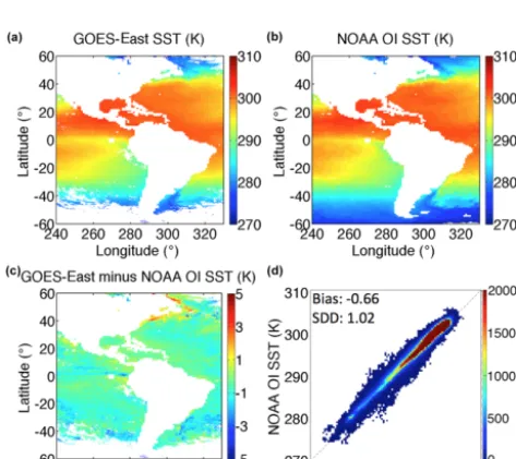
Figure 3 maps the July 2008 SST means from AVHRR (Fig. 3a) and NOAA OI SST (Fig. 3b) as well as their differ-ences (Fig. 3c), which qualitatively reveal very good agree-ment between the two products. The Fig. 3d scatter density plot reveals a more quantitative analysis of the∼3 million daily cell-to-cell comparisons. The bias and standard devia-tion of the difference (SDD) of the AVHRR SST relative to OI SST for July 2008 are−0.06 and 0.62 K, respectively. A high associated coefficient of determination (R2> 0.99; not shown) indicates low variance, despite apparent outliers. Dis-agreements over open ocean, such as those in the tropical western Pacific and northern Pacific Ocean, can be attributed to cloud-clearing differences between the two products or to the fact that the OI satellite SST is supplemented by in situ measurements from buoys and ships that are free of cloud consideration. Nevertheless, despite localized coastal differ-ences and cloud infludiffer-ences, the AVHRR SST is largely con-sistent with the NOAA OI SST product.
Figure 3.July 2008(a)AVHRR SST,(b)NOAA OI SST,(c)SST difference, and(d)scatter density analysis of∼3 million daily matched grid cells.
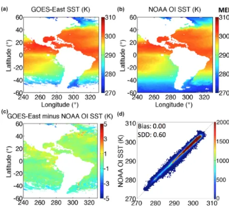
Figure 4.July 2013(a)GOES-13 SST derived, in part, from GFS-based atmospheric corrections,(b)NOAA OI SST,(c)SST differ-ence, and(d)scatter density analysis of∼1 million daily matched grid cells.
is evident from Fig. 5. Figure 5 shows the same compar-ison as Fig. 4, except that MERRA profiles were used for the atmospheric corrections. Similar then to the AVHRR re-trievals, MERRA-derived GOES-13 SSTs exhibit a near-zero bias and an SDD of only 0.60 K relative to the NOAA OI SST reference.
Figure 5. July 2013 (a) GOES-13 SST derived, in part, from MERRA-based atmospheric corrections, (b) NOAA OI SST,
(c)SST difference, and(d)scatter density analysis of∼1 million daily matched grid cells.
5 Land surface temperature angular anisotropy correction
Satellite-observed LST depends on the viewing and illumina-tion condiillumina-tions because shading, vegetaillumina-tion condiillumina-tions, soil type, and topography affect the radiance exiting the scene (Lagouarde et al., 1995; Minnis and Khaiyer, 2000; Minnis et al., 2004). This thermal radiation anisotropy can result in the retrieved LST varying by 6 K or more for some areas (Ras-mussen et al., 2010, 2011; Guillevic et al., 2013). From ex-perimental measurements, Sobrino and Cuenca (1999) and Cuenca and Sobrino (2004) found a viewing zenith angle (VZA) dependence of LST that depends on soil type. Pin-heiro et al. (2006) developed a physical model to estimate the variation of LST as a function of canopy coverage, solar zenith angle (SZA), VZA, and relative azimuth angle (RAA) for a savanna. Rasmussen et al. (2010, 2011) developed and applied a similar model to predict the LST that would be re-trieved by Meteosat over Africa. Vinnikov et al. (2012) con-structed a generalized model to convert satellite-measured, VZA-, SZA-, and RAA-dependent LST into a direction-independent equivalent physical temperature, which for gen-eral application, requires many sets of matched measure-ments from different angle sets to construct coefficients for the necessary kernels. Addressing the anisotropic effects and thereby reducing theTsuncertainties could improve climate monitoring and be of significant benefit to data assimilation and numerical weather prediction needs (Reichle et al., 2010; Guillevic et al., 2013; Draper et al., 2015).
Accounting for 3-D radiance anisotropy for a global re-trieval methodology will require the development of regional
Figure 6.AVHRR (2008) and GOES-13 (2013) SST accuracy and precision relative to NOAA OI SST. For the GEO retrievals, the at-mospheric correction is based on either GFS or MERRA reanalysis. Atmospheric corrections for AVHRR retrievals are strictly based on MERRA.
and seasonal kernels for a universal model (e.g., Vinnikov et al., 2012) or developing canopy configurations globally for physical models (e.g., Rasmussen et al., 2010). Such endeav-ors require many different matched datasets for a sufficiently large configuration of viewing/illumination angle combina-tions across many scene types and all seasons. Therefore, at present, we choose to employ the Vinnikov et al. (2012) universal empirical model for angular anisotropy correction. The model, built from varied surface and climate property observations, can serve as a baseline for angular anisotropy correction despite its development from a small number of ground sites across a limited viewing range. Therefore, the goal of this section is to independently test the efficacy of the model through use of large-area satellite and indepen-dent ground site LST comparisons. If effective, a universal anisotropic correction model such as this is certainly benefi-cial to NRT global retrieval of satellite-based LST. As with Vinnikov et al. (2012), our initial assessment will start re-gionally, i.e., within the GOES-East and GOES-West satel-lite domains.
5.1 Nadir-normalization model for LST retrieval anisotropy
Vinnikov et al. (2012) formulate the skin temperature at a given set of viewing and illumination angles as
Ts(θ, θo, ϕ)=Tn[1+a (1−µ)+bψ (θ, θo, ϕ)], (8)
al. (2012) chose the functional form of the solar kernel as ψ (θ, θo, ϕ)=sin(θ )cos(θo)sin(θo)
cos(θo−θ )cos(ϕ) , (9)
while coefficientsaandbare determined empirically. Phys-ically, the solar kernel attempts to account for the impact of solar intensity and shadowing, as well as the hotspot effect. At night, the solar kernel is defined as 0, i.e.,ψ (θ,θo≥90◦, ϕ)≡0. The emissivity kernel accounts for the VZA depen-dence of the effective emissivity, which can be due to the VZA variation of the emissivity of a pure surface, the chang-ing combination of scene components (e.g., grass, rocks, tree canopy, mountain slopes, valleys) and their respective tem-peratures as VZA changes, or a combination of the two.
Vinnikov et al. (2012) first estimated the emissivity kernel by determining the coefficientain Eq. (8) at night by match-ing nearly simultaneous GOES-E and GOES-WTs measure-ments with five ground site measuremeasure-ments of LST. The dif-ferences in the VZAs for the two satellites, covering a range of 43 to 66◦, provided the variation inµneeded to perform the regression fit. The solar kernel coefficient for each site was then determined in the same manner using the daytime GOES measurements with the assumption that the emissivity kernel is the same for any hour of the day. This follows if one considers that when the solar kernel is integrated over the en-tire range of RAA (0–360◦), it reduces to zero. Thus, the so-lar kernel, in effect, represents deviations from the emissivity kernel. Thus, features such as the hotspot, which occurs in a solar backscatter position whenθo=θ, are compensated by lower values at a different RAA, typically in shadow, or over a range of RAAs at the same value ofθ (e.g., Minnis et al., 2004). It is possible, therefore, that the emissivity kernel, or VZA correction model, could be determined during the day-time by taking measurements over a sufficient range of SZAs and RAAs at a given VZA. Doing so, however, would require a significantly large number of matched datasets in order to achieve sufficient sample size for every interdependent VZA, SZA, and RAA configuration across different surface types and seasons, and thus is much simpler to accomplish at night. 5.2 GOES-East/West LST comparison
To test the efficacy of the Vinnikov et al. (2012) three-kernel anisotropic correction, differences between the hourly GOES-East (GE) and GOES-West (GW) LST retrievals from July 2013 were computed before and after applying the angu-lar adjustments. Prior to differencing, the 15 min discrep-ancy in the image retrieval at the 3 h synoptic times (00:00, 03:00, . . . , 21:00 UTC) was mitigated by adjusting the GE LST, which is based on images beginning 15 min before the UTC hour, to that UTC hour when the GW image scan be-gan. This approach accounts for the specific GE and GW scanline time discrepancies. The GE data were linearly inter-polated to the GW time using the nearest surrounding syn-optic hours. When those surrounding hours crossed the
sun-rise terminator, no correction was applied because of the day-night discontinuity in LST that occurs shortly after sunrise. Data taken near the terminator (SZA between 80 and 100◦)
were not used. The image times at the non-synoptic hours are nearly identical, so no temporal normalization was required. To minimize calibration differences, the average nocturnal LST difference, 0.08 K, between GOES-13 and 15 within 0.5◦ longitude of 105◦W, which is the bisector of the two views, was computed and added to all GOES-15 values.
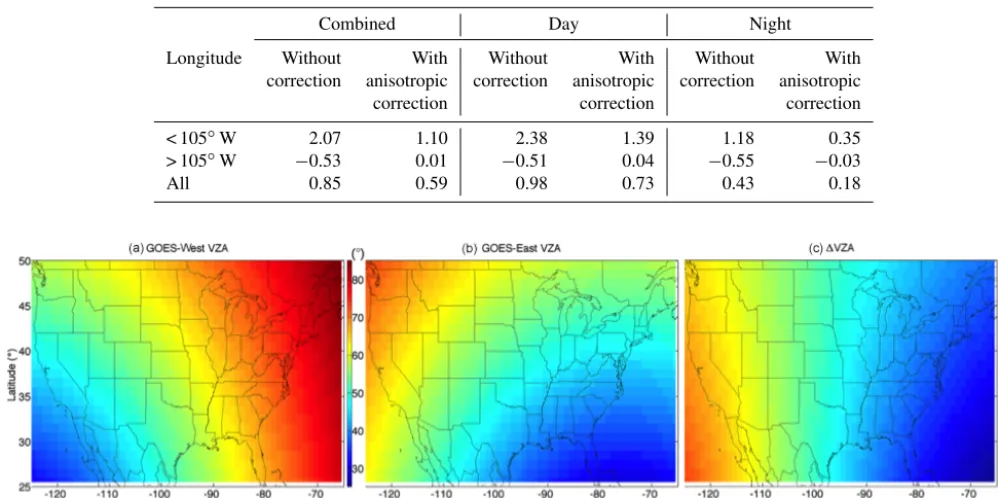
Figure 7 plots the VZAs for GW (Fig. 7a), GE (Fig. 7b), and the GE–GW VZA differences (Fig. 7c). Although the differences are generally less than±30◦, the largest VZAs are up to 70◦ or more. At night, the emissivity kernel from Eq. (8) would suggest large LST differences for pairs matched at the higher VZAs in this domain. All the retrieved values of normalized LST for both satellites were adjusted to nadir to account for the anisotropic dependence.
The mean regional differences, i.e., DTs=LST(GE)−LST(GW), are shown in Fig. 8 for the matched July 2013 data. During daytime, DTs for the unadjusted values (Fig. 8a) is mostly positive east of 105◦W and negative to the west. Notable exceptions include the positive values in the west corresponding the highest mountain ranges in Colorado, Utah, Mexico, Washington, Wyoming, Idaho, and New Mexico. After adjusting to nadir (Fig. 8b), the same patterns remain, but they are mitigated considerably with DTs values closer to zero. Also, the corrected differences for some of the regions at extreme VZAs in the far northeast remain relatively large, perhaps because the viewing dependence increases nonlinearly for large VZA. At night, the unadjusted differences (Fig. 8c) are relatively small, i.e.,|DTs|< 2, in most regions. The positive differences are no longer evident over the high mountains. Applying the anisotropic correction further reduces|DTs|to values less than 1.0 K in nearly all cases (Fig. 8d).
Table 1 summarizes the GE–GW results. Over the east-ern and westeast-ern halves of the domain,|DTs|drops by 0.99 and 0.54 K, respectively, during the day with the application of the anisotropy adjustment. The mean regional differences are much smaller than before correction, especially for the western region where the difference is near zero. Similarly at night, the corresponding regional differences decrease by comparable amounts and are much closer to zero than with-out the corrections. Furthermore, the mean absolute biases for both day and night, which are determined by the east– west sample-weighted region differences (not shown), are much closer after correction – reduced by a factor of 2 or more. Overall, the mean bias for the entire domain after cor-rection over all non-terminator hours is 0.59 K.
Table 1.July 2013 day, night, and combined matched GOES-East minus GOES-West mean clear-sky surface skin temperature difference (K) for regions east and west of 105◦W, without and with anisotropic correction. The sample-weighted average bias is shown in the bottom row.
Combined Day Night
Longitude Without With Without With Without With correction anisotropic correction anisotropic correction anisotropic correction correction correction < 105◦W 2.07 1.10 2.38 1.39 1.18 0.35 > 105◦W −0.53 0.01 −0.51 0.04 −0.55 −0.03 All 0.85 0.59 0.98 0.73 0.43 0.18
Figure 7.Viewing zenith angles for(a)GOES-West and(b)GOES-East, and(c)their differences over the matching domain.
suggests other factors aside from angular anisotropy affect the observed temperatures. It is possible that the solar az-imuthal dependence seen in earlier studies (e.g., Minnis et al., 2004; Vinnikov et al., 2012) is not balanced out for the configurations seen here. The azimuthal dependence includes effects from both the relative solar azimuth angle and the az-imuthal orientation of the terrain and vegetation. Moreover, the heating/cooling rates probably differ between the east-ern and westeast-ern domains because of humidity and altitude differences. Downwelling longwave radiation might play a greater role in the diurnal cycle ofTsin the eastern domain, perhaps diminishing the solar-induced anisotropy. It would be instructive to derive a daytime-specific emissivity kernel over the entire range of RAA in order to test these theories, but as alluded to in the previous subsection, such an endeavor is beyond the purview of this paper, which merely is meant to assess the current anisotropy model, as given by Vinnikov et al. (2012), applied to a large satellite dataset.
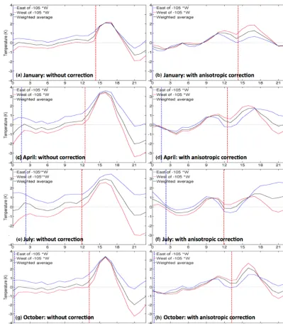
We can, however, explore how DTs changes over the course of a day and how much the anisotropic correction diminishes those differences. To that end, the differences were averaged for each UTC for each of the four months and are plotted in Fig. 9. The July results corresponding to Fig. 8 are plotted in Fig. 9e and f as lines connect-ing the means at each hour. Over the western domain (red line), the uncorrected DTs (Fig. 9e) gradually approaches zero at 09:00 UTC from near −1 K after 03:00 UTC, when
the sun has set over the entire domain. At 12:00 UTC, it rises rapidly to a peak of 2.5 K near 16:00 UTC and drops precipitously after 17:00 UTC to −3 K at 22:00 UTC be-fore increasing until 03:00 UTC. In the east (blue line), DTs drops slowly toward zero after 01:00 UTC but only reaches 0.4 K at 06:00 UTC before increasing again. It only increases significantly after 12:00 UTC, maximizing at 3.5 K (17:00 UTC) before decreasing to 1.3 K at 21:00 UTC, when it levels off. The behavior is rather different for the cor-rected values (Fig. 9f), with the two curves being much closer together between 03:00 and 16:00 UTC, while also being much closer to zero overall than without the angular correction. The corrected western domain DTs rises to near 1.0 K from 09:00 to 11:00 UTC and then drops slightly to about 0.3 K at 12:00 UTC before gradually rising to 1.0 K again by 17:00 UTC. At 17:00 UTC and after, the curves di-verge significantly with the eastern data varying more ex-tremely (rapid and continuous increase from 13:00 through 21:00 UTC) than their western counterparts, suggesting dif-ferent heating/cooling rates. The bias for the entire domain (black line) shows definitively that the afternoon points are mainly responsible for the overall positive bias in Table 1. The results for the other months show that the model gen-erally reduces the mean absolute DTs at most hours. Some exceptions are seen at night.
Figure 8. Mean regional GOES-East–GOES-West LST differences for July 2013.(a)Day without correction,(b) day with anisotropic correction,(c)night without correction, and(d)night with anisotropic correction.
Table 2.Seasonal and diurnal calibration gains for 2013 based on a satellite ray-matching calibration technique described by Minnis et al. (2002). The gain coefficients derive from the ratio of mean GOES-13 and Aqua MODIS time-, space-, and angle-matched radiances, later converted to brightness temperature (BT). A MODIS-consistent GOES-13 BT is attained by multiplying the appropriate gain with GOES-13 BT values. The gains include adjustment for the spectral band difference between the GOES and MODIS channels following the technique described by Scarino et al. (2016). Those spectral band adjustment factor (SBAF) slope and offset values were applied to MODIS BT values (converted from radiance) during the cross-calibration in order to yield MODIS BTs that were spectrally consistent with GOES-13.
January April July October Day Night Day Night Day Night Day Night Calibration gain 0.9998 1.0018 1.0003 1.0027 1.0001 1.0030 1.0007 1.0015 SBAF slope 1.004 1.004 1.006 1.006 1.005 1.005 1.006 1.005 SBAF offset −0.694 −0.708 −1.012 −0.994 −0.867 −0.811 −1.029 −0.952
effects as the surface air and skin temperature equilibrate. Instead of going to zero after 03:00 UTC, DTs drops to roughly −0.8 K for the entire domain by 04:00 UTC until about 06:00 UTC, before rising more rapidly to about 0.8 K at 09:00 UTC and remaining relatively flat until 12:00 UTC. This odd behavior is likely an artifact of the sun–satellite configuration, which causes a change in the infrared channel calibrations at satellite midnight and for 3–4 h afterward. Yu et al. (2013) found that the GOES-11 and GOES-12 10.7 µm (channel 4) brightness temperatures were biased by−0.5 K relative to their daytime calibrations for 3–4 h after satellite
Figure 9.Mean hourly, regional GOES-East–GOES-West LST differences for January, April, July, and October 2013, (left) without and (right) with anisotropic correction. The vertical dashed lines indicate the terminator transitions to night (blue) and day (red) at 37.5◦N, 105◦W.
influenced by the midnight effect. By 07:00 UTC, the smaller GW pre-midnight bias would partially offset the GE bias causing DTs to rise until 09:00 UTC, when only GW is af-fected. After 12:00 UTC, the daylight in the eastern half of the domain would overwhelm any remaining bias. Of course the results discussed here only represent one domain dur-ing one month, although DTs diurnal cycles are shown for other seasonal months in Fig. 9. The midnight calibrations and the viewing/illumination angles vary with time of year. Thus it is clear that a much more comprehensive study would be needed to fully assess the angular anisotropy dependence
of the retrievedTs values in this context. Overall, however, application of the three-kernel model nets meaningful reduc-tion of|DTs| and can perhaps be improved further by in-corporating terrain considerations to account for differential heating/cooling rates.
GOES-Table 3.Bias and SDD values (K) for the GOES-13 and the MYD11 Aqua MODIS product comparison for day, night, and all times combined separated by 2013 seasonal month, without and with the Vinnikov et al. (2012) three-kernel anisotropic correction applied. The numbers in parentheses indicate the sample size for that month.
January (920) April (1992) July (2401) October (1615) Without With Without With Without With Without With correction correction correction correction correction correction correction correction Combined 0.88 0.44 0.85 0.24 1.25 0.25 0.84 0.38 Bias Day 1.34 0.72 1.30 0.49 1.89 0.52 1.69 0.98 Night 0.25 0.08 0.29 −0.07 0.24 −0.13 −0.03 −0.27 Combined 1.79 1.49 1.76 1.28 1.42 1.11 1.90 1.46 SDD Day 2.05 1.71 2.05 1.37 1.07 1.06 2.19 1.45 Night 1.11 1.06 1.05 1.08 1.01 1.03 1.08 1.13
Figure 10.Probability distributions of LST differences from GOES-13 and the MYD11 Aqua MODIS product for day, night, and all times (combined)(a)without and(b)with the Vinnikov et al. (2012) three-kernel anisotropic correction applied, for 2013.
13 10.8 µm channel was first cross-calibrated as in Minnis et al. (2002) against its Aqua MODIS counterpart, band 31, for day and night and the JAJO seasonal months in order to minimize any calibration differences. As part of the cross-calibration, spectral differences were accounted for via con-volution of Infrared Atmospheric Sounding Interferometer (IASI) hyperspectral brightness temperature measurements over the GOES-13 and Aqua MODIS 11 µm channel spec-tral response functions, as thoroughly detailed by Scarino et al. (2016). The diurnal/seasonal calibration coefficients and spectral band adjustment factors (SBAF) are provided in Ta-ble 2. For each Aqua overpass, the MYD11 pixel LST val-ues are converted to pixel radiance and are averaged on the 1◦×1◦GOES-East domain. The mean radiance values are then converted to mean LST and matched to within 15 min of the GOES-13 hourly scans, provided there are at least 150 valid MODIS and GOES-13 pixels per grid cell. To elimi-nate any differences due to surface emissivity discrepancies, the GOES-13 LST was retrieved using the MYD11 band 31 emissivity values. To effect the comparisons, both the
GOES-13 and MYD11 LST values were normalized to the nadir view using Eq. (8).
Figure 10 shows histograms of the differences between the GOES-13 and MYD11 LSTs without (Fig. 10a) and with (Fig. 10b) the Vinnikov et al. (2012) anisotropic correction. Without correction, the GOES LSTs tend to be greater than their MYD11 counterparts, especially during the day. The SDD is greatest during the day at 1.82 K, and the day and night GOES biases are 1.62 and 0.19 K, respectively, result-ing in a combined (both day and night) 0.98 K bias. After applying the anisotropic correction, the daytime SDD drops to 1.33 K, with the bias decreasing by 1.0 down to 0.62 K. The nocturnal bias drops to almost−0.12 K, while its SDD increases slightly from 1.07 to 1.09 K. Although the noctur-nal bias changes sign, the magnitude is less than that prior to the correction.
day-time and combined bias and SDD values reduce substantially following nadir normalization. At night, however, the SDD changes rather subtly and sometimes does not constitute an improvement. In October, for example, the SDD increases from 1.08 to 1.13 K at night, and this is also the only month when the absolute bias increases (−0.03 to−0.27 K). Over-all, the angular anisotropy adjustments reduce the bias by ∼0.7 K, a value resulting from a 1.0 K reduction during the day and ∼0.1 K (0.3 K) absolute (total) reduction at night. The overall SDD dropped by 23 % comprised of a 27 % day-time reduction and a 2 % increase at night. Thus although the emissivity kernel is based on nighttime data, these results indicate that its use to derive the daytime adjustment coeffi-cients is built on a sound assumption of diurnal applicability. The inconsistency at night, especially in October, may be a result of the limited range of viewing angles used to construct the emissivity kernel, although it is perhaps more likely due to nighttime calibration artifacts (e.g., discussion of Fig. 9) that have not yet been fully resolved (Yu et al., 2013).
Similar results (not shown) were found for the GOES-13 LST values retrieved using GFS instead of MERRA. Unlike the SST comparisons (Figs. 4 and 5), the GFS-derived GOES LST bias and SDD values are comparable to those based on the MERRA profiles. Without applying the anisotropic correction, the daytime and nocturnal biases for GOES/GFS retrievals relative to MYD11 are 1.69±1.99 and 0.22±1.12 K, respectively, which are higher, but not sig-nificantly worse than the corresponding MERRA values. Af-ter applying the VZA adjustment, the day and night biases are 0.76±1.43 and−0.11±1.13 K, respectively. Although the GFS results over land, compared to those over ocean, are much closer to those from MERRA, the MERRA-based results are slightly more accurate, relative to MYD11, than their GFS counterparts.
5.4 Validation with ARM SGP infrared thermometer
To obtain estimates of the LST bias and SDD relative to ARM IRT measurements, only confidently clear pixels that include the ARM SGP site were selected from the 2013 GOES-13, GOES-15, and NOAA-19 AVHRR retrievals. In order to minimize the chance of cloud mask errors and edge effects, all adjacent pixels were required to be clear. Fig-ure 11 shows the scatterplots of LST retrieved from the ARM SGP IRT and from matched GOES and AVHRR data. The IRT is a down-looking instrument that measures the up-welling radiating temperature of the ground surface, so it is considered to have a nadir view for this comparison. The points (Fig. 11a) tend to parallel the line of agreement but are mostly above it. The IRT values are 1.07 K greater than their satellite counterparts, on average, with an SDD of 1.94 K. The points corrected for anisotropy (Fig. 11b) are scattered about the line of agreement and the average difference is 0.11 K with SDD=1.91 K. Given that agreement improves comparably for day as well as night further supports the
as-sumption that the night-based emissivity kernel is valid dur-ing all hours of the day.
This improvement for both halves of the diurnal cycle is easier to see in Fig. 12, which plots histograms of the differ-ences, SatCORPS–IRT, before (Fig. 12a) and after (Fig. 12b) anisotropic correction. The daytime bias approaches zero, moving from−0.94±2.41 to 0.09±2.38 K, while the noc-turnal bias changes from −1.18±1.37 to 0.13±1.34 K. When only the GOES data are considered, the corrected data yield 0.16±2.24 and 0.15±1.18 K for day and night, respectively, and when only the AVHRR results are con-sidered, the respective day and night corrected data yield −0.13±2.79 and 0.06±1.75 K. The GOES data were also analyzed using the GFS atmospheric profiles and yielded smaller absolute biases compared to their MERRA counter-parts (−0.85 and −1.10 K for day and night, respectively) for no anisotropic correction. With the correction, the day and night measurements exhibit biases of 0.24 and 0.39 K, respectively, and when combined yield an overestimate of 0.32±1.75 K. This bias is larger than the MERRA-based GOES Only retrievals, but the SDD is reduced by 2.2 %. Thus, the overall accuracy is similar for the two vertical profile sources for this location. Because the MERRA and GFS biases differ significantly for SSTs (Fig. 6), use of the MERRA profiles for retrievingTswith a single IR channel is preferable. See Table 4 for a summary of all results discussed in this section. For any post-adjustment value in Table 4, with the exception of daytime ALL and AVHRR Only SDD, the individual day and night MERRA- or GFS-sourced bias and precision values are within the GOES-R specifications of 2.5 and 2.3 K, respectively (Yu et al., 2012b).
Table 4.Mean bias and SDD values (K) based on results relative to the ARM IRT before and after anisotropic correction using only GOES data, only 2013 AVHRR data, and using combined 2013 GOES and AVHRR results (All). GOES SatCORPS retrievals are based on MERRA (top) and GFS (bottom) input.
GOES GOES corrected AVHRR AVHRR corrected All All corrected MERRA Bias SDD Bias SDD Bias SDD Bias SDD Bias SDD Bias SDD Combined −1.13 1.84 0.16 1.79 −0.80 2.20 −0.02 2.23 −1.07 1.94 0.11 1.91 Day −0.93 2.30 0.16 2.24 −0.88 2.75 −0.13 2.79 −0.94 2.41 0.09 2.38 Night −1.32 1.19 0.15 1.18 −0.74 1.75 0.06 1.75 −1.18 1.37 0.13 1.34 GFS Bias SDD Bias SDD
Combined −0.98 1.76 0.32 1.75 Day −0.85 2.19 0.24 2.17 Night −1.10 1.29 0.39 1.29
Figure 11.Scatterplots of clear-sky surface skin temperatures from 2013 GOES-13, GOES-15, and AVHRR imagery, matched with ARM SGP IRT temperatures(a)without and(b)with anisotropic correction.
5.5 Spatial homogeneity of LST
The biases in the results can be due to many factors, in-cluding errors in the assumed surface emissivities, the at-mospheric profiles, and the surface observations themselves. The representativeness of the site for the much larger area is also potentially a large source of bias. This issue, some-times called the scaling, or up-scaling, problem (Wang and Liang, 2009; Guillevic et al., 2012, 2014; Li et al., 2013), is a concern for any ground-based satellite LST validation effort, but no attempt is made here to up-scale the ground station point observations to fully characterize the relatively large pixel area of the satellite product. The potential impact of the large scale is important to mention, however. For exam-ple, Wang and Liang (2009) conclude that it is not possible to compare satellite-derived LST relative to a single ground LST measurement without introducing bias. Guillevic et al. (2014) discuss that although ground-based LST measure-ments are in most cases suitable for “well-defined and dedi-cated sites”, investigative procedures into measurement
per-formance should be employed when spanning the full range of surface types and conditions surrounding the site. In both studies, high-resolution ASTER data were used to assess the degree of heterogeneity of LST around field stations and evaluate the spatial representativeness for ground-based mea-surements. Heidinger et al. (2013), who forewent up-scaling, bring attention to potentially underestimated errors caused by the scaling uncertainty. Furthermore, Fang et al. (2014), in their non-scaled validation study with SURFRAD and ARM, acknowledge the need to better characterize the uncertainties of comparing point measurements with pixel observations. This need was also recognized by Pinker et al. (2009) and led Fang et al. (2014) to suggest using ASTER or MODIS. Therefore, as similarly cautioned by Heidinger et al. (2013), we advise users to be mindful of the scaling-based uncertain-ties of these non-scaled LSTs. To that end, the remainder of this section aims to quantify the spatial variability of LST surrounding the ARM site.
Figure 12.Probability distributions of LST differences between satellite (GOES-13, GOES-15, and AVHRR) and ARM IRT(a)without and
(b)with anisotropic correction.
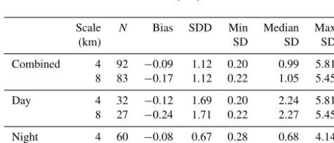
Table 5.Spatial homogeneity assessment of LST (K) using aggre-gates of 45×45 (4 km) and 89×89 (8 km) ASTER pixels at 90 m resolution centered on the ARM SGP Central Facility for day, night, and combined times, using data from 2001 through 2015. The bias and SDD indicate the mean difference and standard deviation of the difference, respectively, of the ASTER central pixel relative to the 4.05×4.05 or 8.01×8.01 km2average. Bias and SDD are based on granulesN, which indicates the number of aggregates where at least 95 % of the 90 m pixels signified clear-sky conditions with no known defects and also represents the number of ASTER granules used to determine the region’s minimum, median, and maximum values of LST standard deviation (SD).
Scale N Bias SDD Min Median Max (km) SD SD SD
Combined 4 92 −0.09 1.12 0.20 0.99 5.81 8 83 −0.17 1.12 0.22 1.05 5.45
Day 4 32 −0.12 1.69 0.20 2.24 5.81 8 27 −0.24 1.71 0.22 2.27 5.45
Night 4 60 −0.08 0.67 0.28 0.68 4.14 8 56 −0.14 0.69 0.30 0.79 5.16
to measure the spatial variance of LST in both a 4×4 and 8×8 km2area centered on the ARM SGP Central Facility. Spatial homogeneity is evaluated in two ways. First, the 4 or 8 km (actually 4.05 and 8.01 km) LST mean (computed from mean radiance and AST_05 surface emissivity) is compared to the central pixel. Second, the heterogeneity is assessed us-ing the minimum, median, and maximum standard deviations (SD) of the 45×45 or 89×89 pixel area, an approach sim-ilar to the method Guillevic et al. (2014) employed for eval-uating a 1 km region centered on various SURFRAD sites. Note that it is not our aim to assess the accuracy of the ASTER product but instead only the consistency of the
large-area and central pixel measurements centered on the ARM site. For such an evaluation, therefore, measurements from ARM are irrelevant. The similarities of the values from the various scales determine the scaling consistency relative to a given ARM SGP measurement.
Results of the ARM spatial homogeneity analysis are pre-sented in Table 5, whereN indicates the number of ASTER granules for which at least 95 % of the pixels signified clear-sky conditions with no known defects. Whether day, night, or combined, the magnitude of the mean difference between the 4 km mean LST and central-pixel LST is near 0.1 K (0.12, 0.08 and 0.09 K, respectively), with the central pixel being slightly cooler in all cases. Although it is true that daytime LST exhibits higher uncertainty than that of nighttime (as also observed by Wang and Liang, 2009, and Guillevic et al., 2014), the SDDs of 1.69, 0.67, and 1.12 K are within the respective GOES Only day, night, and combined post-adjustment precision values of 2.24, 1.18, and 1.79 K. The same can be said for the median SDs, although the daytime value matches the 2.24 K precision exactly. It is therefore concluded that our GOES LST retrievals are too warm rel-ative to the ARM measurement by about 0.1 K on average, which is a minor bias adjustment, with an associated uncer-tainty not in excess of the stated precision values. These val-ues are consistent to the results when considering the 100 % clear granules, in which caseN=9, and the absolute mean bias and uncertainty are 0.12±0.75 K, and median SD is 0.57 K in a range from 0.20 to 2.40 K (not shown). Interest-ingly, although the error is not significantly large, reducing the anisotropy-corrected GOES LST by 0.1 K would bring GOES more in line with the measurements from ARM with both day and night mean biases closer to zero.
dis-parity, e.g., theoretical situations where the ground site is sit-uated near the corners of the containing GOES pixel. The result is a near doubling of the bias to−0.17 K for the com-bined case, which includes a−0.24 K daytime contribution and a −0.14 K nighttime contribution. The SDDs are com-parable to those of the 4 km assessment, which suggests that increasing the aggregation area surrounding the ARM site from 4×4 to 8×8 km2does not significantly influence LST uncertainty. Although the biases are larger in magnitude than those from the 4 km analysis, if they are representative of the expected scaling error between pixel area and the point mea-surement, then, as before, they serve well to adjust GOES LST to match the cooler, on average, ARM measurements. Compared to the 4 km analysis, the median SD values in-creased only slightly to 2.27, 0.79, and 1.05 K for the day, night, and combined cases, respectively. Therefore, as ex-pected, only the daytime SD exceeds the uncertainty deter-mined from the ARM validation results. These results are not meant to suggest that a 4×4 or 8×8 km2area LST is gen-erally representative of any given point measurement within that region. In fact, such cases are certainly unlikely as con-cluded by Wang and Liang (2009) and Guillevic et al. (2014), even for well-known validation sources.
6 Summary and conclusions
Accurate assessment of global climate and improvement of climate models, as well as numerical weather forecasts, rely on consistent land and oceanTs measurements, among oth-ers. Atmospheric flux calculations depend on the robustness of such surface variables, and NWP analyses are driven by reliable and frequent state variable updates over large spa-tial domains. Despite key downsides, satellite data are ideal sources ofTsgiven their model-ready retrieval schedule and broad continuous areal coverage. Thermal-infrared-derived Tsrelies on accurate cloud clearing, atmospheric adjustment, and angular anisotropy consideration. Therefore, validation of satellite Ts relative to known standards is of critical im-portance.
The SatCORPS provides aTsproduct retrieved from GEO and AVHRR sources using the same single-channel algo-rithm. The benefit of the single-channel approach is that this method is more universally applicable to historic and fu-ture satellite instruments compared to the split-window tech-nique. Having GEO and AVHRRTsvalues derived from the same algorithm reduces relative uncertainty and, hence, are better able to supplement one another. Validation of SST retrieved from both satellites demonstrates consistent accu-racy and precision results of less than 0.1 and 0.6 K rela-tive to NOAA OI SST, respecrela-tively, for atmospheric correc-tions based on MERRA profiles. If GFS temperature and hu-midity profiles are used to account for atmospheric attenua-tion, however, the accuracy and precision values for the GEO SST exceed 0.6 and 1.0 K, respectively. The larger negative
bias and precision relative to the MERRA-based results sug-gests that the GFS atmosphere is drier than MERRA over the oceans, on average. This result is surprising in that satel-lite (Tian et al., 2013) and radiosonde (Kennedy et al., 2011) comparisons indicate that MERRA is too dry at altitudes be-low 500 hPa.
Daytime LST retrievals can be significantly influenced by satellite and solar viewing geometry. One must therefore account for this 3-D radiance anisotropy dependence on a global scale in order to create an accurate and uniform prod-uct. Creating a universal model such as this, however, will require the development of regional and seasonal kernels, which requires many different matched datasets for a suf-ficiently large configuration of viewing/illumination angle combinations across many scene types and all seasons. Such an endeavor is left for future work. Here, we have employed the Vinnikov et al. (2012) universal empirical model for an-gular anisotropy correction. It was developed and tested us-ing a very limited set of measurements taken at only five sites over the United States but had not been exercised over a larger scale prior to this study. This article has highlighted independent tests of model effectiveness via large-area satel-lite LST comparisons and ground site validation, which ef-fectively demonstrate the benefit of applying this anisotropic correction to LST retrievals over much of North American in all seasons.
Land surface temperatures retrieved from July 2013 matched GOES-East and GOES-West data over North Amer-ica showed distinct VZA-dependent differences. Normaliza-tion of the daytime LSTs to the nadir view using the Vin-nikov et al. (2012) anisotropic correction model reduced the absolute bias by a factor of 2. The remaining daytime dif-ferences are likely due to differential heating/cooling rates and topographical orientations, which can be potentially mit-igated in the future by implementing terrain and vegetation considerations into the correction model. The GE–GW aver-age nocturnal absolute LST difference is∼0.4 K. Applying the anisotropic correction reduces the mean absolute bias to ∼0.2 K. Overall, application of the three-kernel model nets meaningful improvement despite a need for better terrain handling and more comprehensive study of near-midnight calibration effects for GOES satellites.
bias and precision to 0.34 and 1.36 K, respectively. Compar-isons with LSTs from the ARM IRT ground station provide further evidence of the validity of the SatCORPS retrieval approach and the application of the anisotropic correction, both for day and night. On average, MERRA-based atmo-spheric corrections seem to perform slightly better than GFS-based attenuation for LST retrievals compared to surface and other satellite LSTs. This finding, however, should not re-strict use of GFS for LST retrievals, as the differences are rather small and not strictly better/worse in all scenarios. For SST validation, the MERRA atmosphere is clearly preferred. The small improvements in bias and SDD relative to both the ARM and MYD11 validation efforts (1) demonstrate that large-scale application of the three-kernel LST adjustment for anisotropic dependencies will yield a more accurate and consistent product and (2) support the assumption of diurnal efficacy of the night-based emissivity kernel.
Further investigation is necessary for the ARM ground-site validation approach, particularly in terms of the up-scaling problem. However, a spatial homogeneity analysis using ASTER data at 4 and 8 km scales demonstrated that the average scaling error is small. Also, SD of LST surrounding the ARM measurement site only exceeded determined pre-cision values for daytime granules, which highlights the im-portance of robust solar angle considerations in the satellite retrievals. Regardless, disparity between pixel- and ground-station-observed surface conditions and model sounding de-ficiencies are the likely contributors to the surface–satellite differences. Beyond the outlier cases, however, the corrected SatCORPS GEO and AVHRRTsexhibit minimal mean bias along with high precision. The anisotropic correction, with an adjustment magnitude of ∼1.0 K, affords reductions of 0.8 K and 1 % in absolute LST bias and SDD, respectively. These small reductions yield mean bias and precision values of 0.1 and 1.9 K, respectively, compared to the ground site reference.
This study has examined data from only one small part of the Earth using a single anisotropic model developed using a limited range of viewing angles. It appears to work quite well for the larger domain (central North America), which included the sites used in its development, but there remain several areas for future testing and improvement. The impact of such corrections should be tested over other areas of the globe having different vegetation and terrain. The simple lin-ear emissivity kernel under-corrects at higher VZAs, indicat-ing that a higher-order formulation may be needed. Biases in mountainous areas stand out even after correction, suggest-ing that terrain orientation and morphology may introduce additional complexity in the anisotropy. Regional determi-nation of the Vinnikov et al. (2012) model coefficients may be ideal, but deriving those coefficient values would require many matched datasets to achieve sufficient sampling at a large variety of VZA, SZA, and RAA combinations across all seasons, a task that is left for future work. Because land areas are viewed at fixed VZAs by GEO imagers, the LST
retrievals will suffer from VZA biases and, at a given local hour, solar illumination biases. Removal of those biases will improve the quality of LST monitoring and enhance the util-ity of these datasets for assimilation into numerical weather models. Therefore, incorporating these anisotropic correc-tions for LST into the near-global NRT retrievals, for over-lapping GEO and LEO imagers with robust cloud screening algorithms, will benefit the data assimilation and climate re-search communities and hopefully lead to improved forecasts and better understanding of the global climate system.
7 Data availability
The GEO satellite skin temperature data can be accessed at http://satcorps.larc.nasa.gov/, whereas the AVHRR data are available at https://gis.ncdc.noaa.gov/all-records/catalog/ search/resource/details.page?id=gov.noaa.ncdc:C00876. The angular corrections reported here have not been applied to the current versions of those datasets.
Competing interests. The authors declare that they have no conflict of interest.
Acknowledgements. This research was supported by the NASA Modeling, Analysis, and Prediction Program and the NOAA CDR Program. Computing was supported by the NASA High End Com-puting Program. The authors would like to thank Sarah Bedka and Doug Spangenberg for their generous assistance with SatCORPS processing.
Edited by: M. Portabella
Reviewed by: I. Trigo and two anonymous referees
References
Bodas-Salcedo, A., Ringer, M., and Jones, A.: Evaluation of the surface radiation budget in the atmospheric component of the Hadley Centre Global Environmental Model (HadGEM1), J. Cli-mate, 17, 4723–4748, 2008.
Bosilovich, M., Radakovich, J., Silva, A. D., Todling, R, and Verter, F.: Skin temperature analysis and bias correction in a coupled land-atmosphere data assimilation system, J. Meteorol. Soc. Jpn., 85, 205–228, 2007.
Chen, Y., Sun-Mack, S., Minnis, P., Young, D. F., and Smith Jr., W. L.: Seasonal surface spectral emissivity derived from Terra MODIS data, Proc. 13th AMS Conf. Satellite Oceanogr. and Me-teorol., Norfolk, VA, 20–24 September, CD-ROM, P2.4, 2004. Chen, Y., Minnis, P., Sun-Mack, S., Arduini, R. F., and Trepte, Q. Z.:
Clear-sky and surface narrowband albedo datasets derived from MODIS data, Proc. AMS 13th Conf. Atmos. Rad. and Cloud Phys., Portland, OR, June 27–July 2, JP1.2., 2010.
Coll, C., Wan, Z., and Galve, J. M.: Temperature-based and radiance-based validations of the V5 MODIS land sur-face temperature product, J. Geophys. Res., 114, D20102, doi:10.1029/2009JD012038, 2009.
Cuenca, J. and Sobrino, J.: Experimental measurements for study-ing angular and spectral variation of thermal infrared emissivity, Appl. Opt., 43, 4598–4602, doi:10.1364/AO.43.004598, 2004. DaCamara, C. C.: The Land Surface Analysis SAF: One year of
pre-operational activity, in: Proc. 2006 EUMETSAT Meteorol. Satellite Conf., Helsinki, Finland, 2006.
Draper, C., Reichle, R., De Lannoy, G., and Scarino, B.: A dynamic approach to addressing observation-minus-forecast mean differ-ences in a land surface skin temperature data assimilation system, J. Hydrometeorol., 16, 449–464, 2015.
Environmental Modeling Center: The GFS Atmospheric Model, NCEP Office Note 442, Global Climate and Weather Modeling Branch, EMC, Camp Springs, Maryland, 2003.
Duan, S.-B., Li, Z.-L., Tang, B.-H., Wu, H., Tang, R., Bi, Y., and Zhou, G.: Estimation of diurnal cycle of land surface temperature at high temporal and spatial resolution from clear-sky MODIS data, Remote Sens., 6, 3247–3262, 2014.
Fang, L., Yu, Y., Xu, H., and Sun, D.: New retrieval algorithm of de-riving land surface temperature from geostationary orbiting satel-lite observations, IEEE T. Geosci. Remote, 52, 819–828, 2014. Garand, L.: Toward an integrated land-ocean surface skin
temper-ature analysis from the variational assimilation of infrared radi-ances, J. Appl. Meteorol., 42, 570–583, 2003.
Ghent, D., Kaduk, J., Remedios, J., Ardö, J., and Balzter, H.: Assim-ilation of land surface temperature into the land surface model JULES with and ensemble Kalman filter, J. Geophys. Res., 115, D19112, doi:10.1029/2010JD014392, 2010.
Göttsche, F. M., Olesen, F. S., and Bork-Unkelbach, A.: Validation of land surface temperature derived from MSG/SEVIRI with in-situ measurements at Gobabeb, Namibia, Int. J. Remote Sens., 34, 3069–3083, 2013.
Gillespie, A., Rokugawa, S., Matsunaga, T., Cothern, J. S., Hook, S., and Kahle, A. B.: A temperature and emissivity separation algorithm for Advanced Spaceborne Thermal Emission and Re-flection Radiometer (ASTER) images, IEEE T. Geosci. Remote, 36, 1113–1126, 1998.
Goody, R., West, R., Chen, L., and Crisp, D.: The correlated-k method for radiation calculations in nonhomogeneous atmo-spheres, J. Quant. Spectrosc. Ra., 42, 539–550, 1989.
Guillevic, P. C., Privette, J. L., Coudert, B., Palecki, M. A., De-marty, J., Ottlé, C., and Augustine, J. A.: Land surface tempera-ture product validation using NOAA’s surface climate observa-tion networks – Scaling methodology for the Visible Infrared Imager Radiometer Suite (VIIRS), Remote Sens. Environ., 124, 282–298, 2012.
Guillevic, P. C., Bork-Unkelbach, A., Göttsche, F. M., Hulley, G., Gastellu-Etchegorry, J-.P., Olesen, F. S., and Privette, J. L.: Di-rectional viewing effects on satellite land surface temperature products over sparse vegetation canopies – A multisensor analy-sis, IEEE T. Geosci. Remote, 10, 1464–1468, 2013.
Guillevic, P. C., Biard, J. C., Hulley, G. C., Privette, J. L., Hook, S. J., Olioso, A., Göttsche, F. M., Radocinski, R., Romàn, M. O., Yu, Y., and Csiszar, I.: Validation of land surface temperature products derived from the Visible Infrared Radiometer Suite
(VI-IRS) using ground-based and heritage satellite measurements, Remote Sens. Environ., 154, 19–37, 2014.
Heidinger, A. K., Laszlo, I., Molling, C. C., and Tarpley, D.: Using SURFRAD to verify the NOAA single-channel land surface tem-perature algorithm, J. Atmos. Ocean. Technol., 30, 2868–2884, 2013.
Jiménez-Muñoz, J. C., and Sobrino, J. A.: A single-channel algo-rithm for land-surface temperature retrieval from ASTER data, IEEE Geosci. Remote S., 7, 176–179, 2010.
Jiménez, C., Prigent, C., Catherinot, J., Rossow, W., and Liang, P. A.: Comparison of ISCCP land surface temperature with other satellite and in situ observations, J. Geophys. Res., 117, D08111, doi:10.1029/2011JD017058, 2012.
Jin, Z., Charlock, T. P., Rutledge, K., Stamnes, K., and Wang, Y.: Analytical solution of radiative transfer in the coupled atmosphere-ocean system with a rough surface, Appl. Opt., 45, 7443–7455, 2006.
Kabsch, E., Olesen, F. S., and Prata, F.: Initial results of the land surface temperature (LST) validation with the Evora, Portugal ground-truth station measurements, Int. J. Remote Sens., 29, 5329–5345, 2008.
Kennedy, A. D., Dong, X., Xi, B., Xie, S., Zhang, Y., and Chen, J.: A comparison of MERRA and NARR reanalyses with the DOE ARM SGP data, J. Climate, 24, 4541–4557, 2011.
Kerr, Y. H., Lagouarde, J. P., Nerry, F., and Ottlé, C.: Land sur-face temperature retrieval: Techniques and applications: Case of the AVHRR, in: Thermal Remote Sensing in Land Surface Pro-cesses, edited by: Quattrochi, D. A. and Luvall, J. C., CRC Press, 2004.
Kratz, D. P.: The correlated k-distribution technique as applied to the AVHRR channels, J. Quant. Spectrosc. Ra., 53, 501–507, 1995.
Lagouarde, J. P., Kerr, Y. H., and Brunt, Y.: An experimental study of angular effect on surface temperature for various plant canopies and bare soils, Agr. Forest Meteorol., 77, 167–190, doi:10.1016/0168-1923(95)02260-5, 1995.
Lazzara, M. A., Benson, J. M., Fox, R. J., Laitsch, D. J., Rueden, J. P., Santek, D. A., Wade, D. M., Whittaker, T. M., and Young: J. T.: The Man computer Interactive Data Access System: 25 years of interactive processing, B. Am. Meteorol. Soc., 80, 271–284, 1999.
Li, Z.-L., Tang, B.-H., Wu, H., Ren, H., Yan, G., Wan, Z., Trigo, I. F., and Sobrino, J. A.: Satellite-derived land surface temperature: Current status and perspectives, Remote Sens. Environ., 131, 14– 37, 2013.
Minnis, P. and Khaiyer, M. M.: Anisotropy of land surface skin temperature derived from satellite data, J. Appl. Meteorol., 39, 1117–1129, 2000.
Minnis, P., Nguyen, L., Doelling, D. R., Young, D. F., Miller, W. F., and Kratz, D. P.: Rapid calibration of operational and research meteorological satellite imagers, Part II: Comparison of infrared channels, J. Atmos. Ocean. Technol., 19, 1250–1266, 2002. Minnis, P., Gambheer, A. V., and Doelling, D. R.: Azimuthal
anisotropy of longwave and infrared window radiances from CERES TRMM and Terra data, J. Geophys. Res., 109, D08202, doi:10.1029/2003JD004471, 2004.