Bayesian Analysis of the Weibull lifetimes under type-I Ordinary Right Censored Samples

Bayesian Analysis of the Weibull Lifetimes under

Type-I Ordinary Right Censored Samples

Muhammad Saqib

College of Statistical and Actuarial Sciences University of the Punjab, Lahore, Pakistan [email protected]

Irum Sajjad Dar

College of Statistical and Actuarial Sciences University of the Punjab, Lahore, Pakistan [email protected]

Abstract

Censoring is an unavoidable feature of reliability and survival analysis due to time and cost constraints. In this paper, we numerically study the effect of sample size, censoring rate and parameter size of Weibull distribution on its estimates. Some interesting properties and comparison of the Bayes and ML estimates along with their standard errors have been studied. The sample expressions for the Bayes and ML estimates and their variances are derived as a function of test termination time. The difference between ML estimates and uninformative Bayesian estimates becomes negligible for large sample size.

Keywords: Censored Data, Inverse transformed method, Fixed test termination time, Uniform Prior.

1. Introduction

In recent era Weibull distribution has proved its importance in the field of reliability and life testing because of its flexibility in fitting life time distributions. Various problems associated with this distribution have been considered by numerous writers, among whom are Kao (1958, 1959), Leone, Rutenberg, and Topp (1960), Procassini and Romano (1961), Lloyd and Lipow (1962), Dubey (1963), Esary and Proschan (1963), Lehman (1963), Menon (1963), Proschan (1963) and Jaech (1964).

Seguro and Lambert (2000) proposed modified maximum likelihood method to calculate the parameters of the Weibull wind speed distribution for wind energy analysis. They recommended their method for use with wind data in frequency distribution format. Ng et al. (2012) used maximum likelihood estimators (MLEs), corrected MLEs, weighted MLEs, maximum product spacing estimators and least squares estimators to estimate three parameter Weibull distribution based on progressively Type-II right censored sample. In addition they proposed the use of a censored estimation method with one-step bias-correction to obtain estimates for iterative procedures.

Saleem and Aslam (2010a) focused on rayleigh distributed survival time with a rayleigh distributed censor time considered to derive the maximum likelihood and the Bayes estimators for the unknown parameters and their corresponding variances. Saleem et al. (2010b) considered the Bayesian analysis of the mixture of power function distribution using the complete and the censored sample. The characteristic function of three parameter Weibull distribution is derived independently and the moment generating function (MGF) is deduced from it by Muraleedharan (2013). It generated all the moments of the distribution and satisfies the tests to verify a function to be a characteristic function. He also obtained expressions for mean, variance, skewness and kurtosis from MGF. Further literature on parameter estimation is available in Munir et al. (2013).

A major deterrent to wider usage of the Weibull distribution has been the difficulty in estimating its parameters. Unfortunately, the calculations involved are not always simple. Depending on the values of the parameters, the Weibull distribution can be used to model a variety of life behaviors. It is a versatile distribution that can take on the characteristics of other types of distributions, based on the value of the shape parameter.

2. The Weibull distribution

The two-parameter Weibull random variable t has the following distribution function







       

 



 

t e t

F ; , 1 ; t0 ₍₁₎

and the density function is given by





_ _ _

     

  



   

t

e t t

f ; , 1 ; t0 ₍₂₎

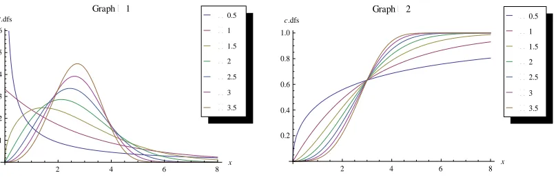
Here; v0 is the shape parameter and  0 is the scale parameter of the distribution. Its complementary cumulative distribution function is a stretched exponential function. The Weibull distribution is related to a number of other probability distributions, it interpolates between the exponential distribution (v1) and the Rayleigh distribution (v2).

Figure 1: Shows some of the simple Weibull distribution for  3.

Graphical representations of different values of shape parameter for the Weibull model are shown in figure-1. This figure suggests that as we increases the shape parameter the distribution tends to be approximately normal. However, for higher values of shape parameter the graph of cdf gives elongated S shape for the Weibull model.

Table 1: Parameters affect on properties of Weibull distribution Parameters

Descriptives Skewness Kurtosis Condition Range

Mean< Variance

Positive Leptokurtic

Mean = Variance

Mean >Variance

Pletykurtic Negative

Mean< Variance

Positive Leptokurtic

Mean >Variance

Pletykurtic Negative

--- ---

Positive Leptokurtic

Pletykurtic Negative

Saqib (2014) found some parameters affect on properties of Weibull distribution about table 1 shows that

 when shape & scale parameter are equal

but lies b/w (0, 1) the mean is less than variance and the distribution is positively skewed & leptokurtic. But, when shape & scale parameter are equals to one, the mean is equal to variance and the distribution is positively skewed & leptokurtic. Similarly, when shape & scale parameter lies b/w (1, 2] the mean is greater than variance and the distribution is positively skewed & leptokurtic. However, when shape & scale parameter lies b/w (2, 3.5] the mean is greater than variance and the distribution is positively skewed & pletykurtic. When both parameters are greater than , the mean will be greater than variance and the distribution is negatively skewed & pletykurtic.

2 4 6 8

x 0.1

0.2 0.3 0.4 0.5 0.6 P.dfs

Graph 1

3.5 3 2.5 2 1.5 1 0.5

2 4 6 8 x

0.2 0.4 0.6 0.8 1.0 c.dfs

Graph 2

3.5 3 2.5 2 1.5 1 0.5

v

 

1 , 0 v

1

,v



2 , 1 v

5 . 3 , 2 v

5 . 3 ,v



v

 

1

 v

2

1v

5 . 3

2v

5 . 3

 v

v

 

v  

2

 v

5 . 3

2v

5 . 3

 v

 when scale parameter is greater than shape parameter

but scale parameter is greater than or equal to 4 and shape parameter less than or equal to 1.5, the mean is less than variance and the distribution is positively skewed & leptokurtic. However, if scale parameter is greater than or equal to 4 and shape parameter greater than 1.5, the mean will be greater than variance and the distribution is positively skewed & leptokurtic.

 when scale parameter is less than shape parameter

the mean is greater than variance but if shape parameter less than or equal to 2 the distribution will be positively skewed & leptokurtic. When scale parameter is less than shape parameter, but shape parameter lies between (2, 3.5] the distribution is positively skewed & pletykurtic. If shape parameter is greater than 3.5, the distribution will be negatively skewed & pletykurtic.

3. Methodology

Censoring is an important feature of the lifetime data because most of the times it is not feasible to continue the experiment until the last observation in order to obtain a complete data set, i.e., a data set with the exact life times of all the objects. A censored data set contains at least one observation about which only partial information on the exact failure time is available. There are three types of censored observations, the left, the interval and the right censored observations. A right censored observation may be of Type I or Type II. Censoring is said to be of Type I if the censoring time is fixed and the number of failures is random. On the other hand in Type II, censoring the number of failures in the sample is predetermined and so the time to complete the test is random. Basic literature on account of censoring can be seen in Kalbfleisch and Prentice (2002).

3.1 Sampling

In a typical life test, n samples are placed under observation and as each failure occurs, the time is noted. Finally at some pre-determined fixed time T or after some pre-determined fixed number of sample fail, the test is terminated. In both of these cases the data collected consist of observations t t₁, ,₂ ,tn plus the information that (n – r) samples

survived beyond the time of termination, T in the former case, and tn in the latter. When T

is fixed and r is thus a random variable, censoring is said to be of type I. When r is fixed and the time of termination tn is a random variable, censoring is said to be of type II. We

define t_j failure time of the jth unit belonging to the population where j1,2...r,

T t_j 



0 .

3.2 Censored Likelihood Function

The Likelihood Function for the Weibull distribution is given by;

 



 



_



 _

   

  

 



r n j

r

j f t F T

L 1

1 (3)

Where t_j 



t1,t2,..., t_r



corresponds to sample data.

 

1 1

1 1 ln

r r

v v

j

j j

j

r v t n r T

t

v

L e e 



 

 

  _{    }  _ _{  }    

     

3.3 ML Estimation

Saqib (2014) obtained ML estimates by simultaneously solving the two equations obtained by setting the first order derivatives of the likelihood with respect to  , to zero.

Where (5)

(6)

It is not possible to solve the above system of nonlinear equations analytically. However they can be solved by numerical iterative procedure. Let and it is a well known

result that .

3.4 Variance of ML estimates

For Weibull distribution of our objective elements are given by

(7)

is the information matrix of order , inverting it we can find the variance of ML estimates on the main diagonal. Following are the elements of the symmetric information matrix.

(8)

(9)

(10)

3.5 Expressions for Estimators and Their Variances Assuming Uniform Prior

Let us assume a state of ignorance that  and vare uniformly distributed over



0,



. Hence

 

1, 0

f  k    andf v

 

k₂, 0  v .

Assuming independence we have an improper joint prior that is proportional to a constant and is incorporated with the likelihood (3.4) to yield a proper joint posterior distribution. The respective marginal distributions yield the following Bayes estimators of  and v under the squared error loss function.

Pr

PosteriorLikelihood ior (11)

v v

T r n t

r

r ˆ

ˆ

) ( ˆ 1

ˆ  



 

v j r j v

t t

r ˆ

1 ˆ

  





  

 _{ }  _





 j

r j v

j v j r

j T T t

r n t t v

r ˆ 1_ˆ ln _ˆ ln ln

1 ˆ

ˆ

1 



 

   ,

 



 



 1

, ~N I

 

   

 

   

 

   

  

 

      

 

  

  

2 2 2

2

2 2 2

v l v

l

v l l

E l

E I

  

  

2 2

2

2 2

ln( ) 1 2

[ ( ) v]

L

E r n r T



 

_ 

 _ _  



 

2 2

2 2

] [ln ) ( 1 )

ln(

T T r n v

r v

L

E    v

   

 

  



T T r n v

L E

v L

E ln( ) ln( ) 1₂( ) vln

2 2

 

    

 

        

 

   

 





1 1   1 1 ln 1 1 , | r r v v j j j j

r v t n r T

t r

p v t v e e

c          _{ }      _{   }         _{ }

  ; ,v0 (12)





1





1 1 ln 0 1 1 r j j r v r t

r v v

j j

c r v e  t n r T dv

       _ _            







Now marginal posterior distribution for v

   

1





1 1 ln 1 1 | r j j r v r t

r v v

j j

r

p v t v e t n r T

c    _   _{ }          _   _





 ; 0  v (13)

Now we obtain Bayes estimator and its variance for v under square error loss function.





1





1 1 ln 1 0 1 1 r j j r v r t

r v v

B _j

j

r

v v e t n r T dv

c    _     _  _{ }   _{ }    _   _ 







 

  _{ }   _{ } 1 1 1 1 ln 2 0 1 2 1 1 ln 1 0 1 1 1 r j j r j j r v r t

r v v

j j B r v r t

r v v

j j

r

v e t n r T dv

c V v

r

v e t n r T dv

c     _     _             _ _ _  _{    }   _{    }   _{ }     _{  }         _{ }       _{ }    _{ }   









 









1  

1 1 1 1 | 1 r v v j j r r v v

j _{t n r T}

j

r

t n r T

p t e

r           _   _  _{ }       _     



;   0 (14)

Now we obtain Bayes estimator and its variance for  under square error loss function.

  1 2 B r v v j j

t n r T

r            



 

_ _ _ 2 1 2 3 2 B r v v j j

t n r T V r r             



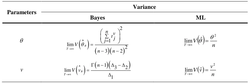
3.5 The Limiting Expression

When the sample is uncensored, T tends to , r tends to n and consequently all the observations are included into our analysis. Therefore, the amount of information contained in the sample is increased, which consequently results in the reduction of the





1

1 1 1 1 ln 1 ₀ 1 1 1 ln 1 2 0 1 1 1 ln 2 3 0 1 1 n j j n j j n j j n v n t n v j j n v n t n v j j n v n t n v j j

n v e t dv

v e t dv

v e t dv

variances of the estimates. The expressions for the complete sample Bayes and ML estimators (table 2) and their variances (table 3) are simplified below.

Table 2: The limiting expressions for the Bayes and ML estimates as T

Parameters Estimator

Bayes ML

 ₁

lim

2

B

n v j j T

t

n  

  



v   2

1

1 lim B

T

n v



   



In Table 2 the efficiency of both (Bayes and ML) estimates are increased. This is clear from the second order derivatives of the log likelihood given in above section that the off diagonal terms of the information matrix vanish and ensure the independence of the ML estimates. The information matrix becomes a diagonal matrix which can very comfortably be inverted by simply inverting the terms on the main diagonal.

Table 3: The limiting expressions for the Bayes and ML variances as T

Parameters

Variance

Bayes ML



 







2 1

lim ₂

3 2

B

T

n _v t j j V

n n





  

 

 

 

 

v lim

 

 1



3 2



1

B

T

n V v



     



4. Simulation Study

A simulation study was conductedin order to investigate the performance of the Bayes estimators, impact of sample size and censoring rate on the fit of the model. Sample of sizes =20, 30, 50, 100, 150, 300 and 500 were generated from the Weibull distribution with parameters v and  such that v=1, 1.5, 2, 2.5 and = 4, 5. A random number u was generated from the uniform on (0, 1) distribution. Right censoring was carried out using a fixed censoring time T. All the observations that were greater than T were declared censored ones. Different fixed censoring times T were chosen in order to evaluate the impact of censoring rates on the estimates. For each of the combination of parameters, sample size and censoring rate, 1000 samples were generated using the Mathemetica following the inverse transformation method of simulation. In each case

n tvj n

j T

ˆ 1

ˆ lim 

 

 



  

 _{ }



 

 

j n

j j v j n j T

t t

t n v

ln ln

ˆ 1 ˆ lim

1 ˆ

1



 

n V

T

2 ˆ

lim  

 

 

n v v V

T

2 ˆ

lim 

only failure units were identified. For each of the 1000 samples, for each of combinations of parameters the Bayes estimates were computed through Mathemetica and average of 1000 estimates is presented in table 4-7.

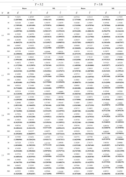
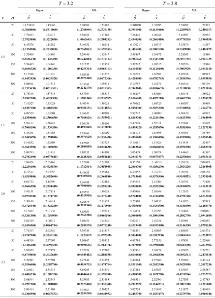
Reference to table 4-5 shape & scale parameter becomes closer to their corresponding lifetime parameters by increasing the sample size for both the techniques. For Bayes estimates, if we increase the values of shape parameter a decrease in estimates of scale parameter is noted but some exceptional cases at different censoring rates for different sample sizes and vise versa whilst there is a mixed pattern is observed in ML estimates. With an increase in the values of scale parameter, table 4 reports, a decrease in estimates of shape parameter is noted at different censoring rates for different sample sizes and vise versa however, there is a mixed pattern is observed in ML estimates. In addition, for Bayes estimates, it is observed that both the lifetime parameters are over estimated but were under estimated also for ML estimates.

The standard errors of Bayes and ML estimates for both the lifetime parameters decreases by increasing sample size (table 4-6) but at different censoring rates the standard error of scale parameter increases with an increase in corresponding lifetime parameter for different sample sizes. It is worth mentioning that by increasing shape parameter the standard error of scale parameter decreases at different sample sizes by varying censoring rates for Bayes estimates but showed mixed pattern in ML estimates. Also, the standard error of shape parameter decreases with an increase in corresponding lifetime parameter for different sample sizes at different censoring rates for Bayes estimation while in ML estimation it increases but some exceptional cases. It is worth mentioning that by increasing scale parameter the standard error of shape parameter increases at different sample sizes by varying censoring rates for Bayes estimates whilst increase but some exceptional cases.

Table 4: Bayes and ML estimates of Weibull parameters and their standard errors (in parenthesis) with



4.

v n

3.2

T T3.8

Bayes ML Bayes ML

ˆ

 vˆ ˆ vˆ ˆ vˆ ˆ vˆ

1.0

20 7.19471

(3.4507800)

1.28707

(0.3741940)

4.51477 (0.9661165)

1.21353 (0.2600462)

6.67216

(2.7179300)

1.25113

(0.3371670)

4.47566 (0.9198310)

1.17355 (0.2265257)

30 5.61429

(1.7499100)

1.16649

(0.2691490)

4.38479 (0.7593076)

1.18479 (0.2086842)

5.44280 (1.5314500) 1.15055 (0.2478760) 4.45548 (0.7587060) 1.15184 (0.1895430)

50 4.88919

(1.0499700)

1.10308

(0.1945050)

4.31858 (0.5841327)

1.11385 (0.1591634)

4.75223 (0.9512690) 1.08416 (0.1800130) 4.43735 (0.5964770) 0.98118 (0.1362210)

100 4.39189

(0.6262320)

1.04570

(0.1293840)

4.24565 (0.4033634)

1.09176 (0.1099555)

4.32869 (0.5805160) 1.04109 (0.1217960) 4.39457 (0.4069010) 1.13167 (0.1013190)

150 4.26180

(0.4869270)

1.03144

(0.1101270)

4.16786 (0.3245027)

1.08560 (0.0908743)

4.20619 (0.4517850) 1.02649 (0.0982475) 4.36875 (0.3303450) 1.12201 (0.0837957)

300 4.09997

(0.3254730) 1.01035 (0.0743993) 4.13779 (0.2262980) 1.08309 (0.0632007) 4.09890 (0.3100450) 1.01357 (0.0714434) 4.24468 (0.2257830) 1.10830 (0.0574355)

500 4.07358

(0.2490030) 1.01019 (0.0601047) 4.03898 (0.1711410) 1.05531 (0.0484285) 4.04530 (0.2473270) 1.01132 (0.0523621) 4.19875 (0.1732940) 1.09484 (0.0444025) 1.5

20 6.30182

(1.9994100)

1.80642

(0.4053070)

4.51148 (0.9376641)

1.51658 (0.2908818)

6.22258

(1.8324500)

1.78143

(0.3673360)

3.62083 (0.7472523)

1.76288 (0.3059064)

30 5.49872

(1.3172500)

1.70978

(0.3129870)

4.38436 (0.7383360)

1.51234 (0.2335151)

5.18556

(1.1489500)

1.66058

(0.2810880)

3.97424 (0.6925077)

1.65220 (0.2633672)

50 4.75701

(0.8325540)

1.61109

(0.2293900)

4.31877 (0.5610562)

1.35772 (0.1670272)

4.66587

(0.7678740)

1.58919

(0.2087880)

4.34749 (0.5633435)

1.37691 (0.1599125) 100 4.34289

(0.5184820) 1.55084 (0.1575360) 4.28988 (0.3913560) 1.55099 (0.1270410) 4.29713 (0.4833970) 1.54317 (0.1449760) 4.22335 (0.3811640) 1.37200 (0.1091100)

150 4.22063

(0.4056480) 1.53649 (0.1279050) 4.23065 (0.3170900) 1.51586 (0.1038450) 4.18661 (0.3800570) 1.52785 (0.1164260) 4.19335 (0.3142090) 1.38568 (0.0934294)

300 4.09519

(0.2744600) 1.51489 (0.1001660) 4.14860 (0.2201680) 1.42809 (0.0709315) 4.08903 (0.2602480) 1.51420 (0.0818803) 4.15246 (0.2206410) 1.39705 (0.0669389)

500 4.05154

(0.2120290) 1.51010 (0.0723765) 4.10455 (0.1682420) 1.44905 (0.0552005) 4.04269 (0.2046760) 1.50196 (0.0507364) 4.10546 (0.1668780) 1.42986 (0.0511211) 2.0

20 6.06587

(1.6209200)

2.35309

(0.4488600)

3.75813 (0.7853611)

1.89356 (0.3486445)

5.91030

(1.5178900)

2.30974

(0.4206920)

4.42746 (0.9138446)

1.94072 (0.3199547)

30 5.20980

(1.0831100)

2.22629

(0.3466050)

4.37385 (0.7401446)

1.96165 (0.2817098)

5.16009 (1.0363400) 2.20033 (0.3271930) 3.79182 (0.6290870) 1.54082 (0.2199580)

50 4.57166

(0.7104900)

2.11499

(0.2568260)

4.29944 (0.5554359)

1.99091 (0.2107952)

4.58713 (0.6887380) 2.10852 (0.2416980) 4.29323 (0.5721330) 1.79729 (0.2076130) 100 4.27054

(0.4565780)

2.06178

(0.1832280)

4.25557 (0.3945821)

1.99970 (0.1566726)

4.30503 (0.4489980) 2.05634 (0.1679510) 4.16022 (0.3912820) 1.98304 (0.1557270)

150 4.19823

(0.3629330)

2.04192

(0.1505890)

4.21657 (0.3158156)

2.20800 (0.1309912)

4.18728 (0.3522340) 2.03410 (0.1354940) 4.15647 (0.3246010) 2.26039 (0.1483010)

300 4.08764

(0.2481610) 2.02392 (0.1021130) 4.04774 (0.2171220) 2.15530 (0.0956315) 4.08196 (0.2457320) 2.01556 (0.0943119) 4.09376 (0.2268670) 2.17403 (0.1038930)

500 4.04346

(0.1892850) 2.01237 (0.0860997) 4.04075 (0.1677230) 2.12299 (0.0731641) 4.05426 (0.1903370) 2.01174 (0.0783425) 4.00993 (0.1717180) 2.17229 (0.0796076) 2.5

20 5.97999

(1.5086900)

2.91652

(0.5204230)

4.42925 (0.9181171)

2.17216 (0.3673513)

5.83774 (1.4629500) 2.87700 (0.5093470) 4.30473 (0.8735970) 2.09302 (0.3140460)

30 5.07120

(1.0036800) 2.75274 (0.3985190) 4.41749 (0.7511210) 2.40950 (0.3239690) 5.18209 (1.0193100) 2.76175 (0.3967640) 3.90556 (0.6583897)

2.09888 (0.27467053)

50 4.54189

(0.6910280)

2.65711

(0.2982060)

4.39638 (0.5879694)

2.55503 (0.2767716)

4.70630

(0.6747300)

2.64981

(0.2939140)

4.41858 (0.5897491)

2.26333 (0.24123598) 100 4.23716

(0.4405630) 2.57199 (0.2035910) 3.96305 (0.3839580) 2.44461 (0.2122710) 4.26042 (0.4366850) 2.56026 (0.2020740) 4.23542 (0.4055380) 2.46391 (0.1926110)

150 4.15945

(0.3463750)

2.54416

(0.1679980)

4.19438 (0.3298788)

2.43035 (0.1680274)

4.21628 (0.3502970) 2.54928 (0.1629970) 4.16473 (0.3273520) 2.62957 (0.1686170)

300 4.08455

(0.2388020)

2.52293

(0.1200320)

4.04033 (0.2259296)

2.47233 (0.1233888)

4.07404 (0.2370330) 2.51909 (0.1143040) 4.13336 (0.2337750) 2.59408 (0.1314690)

500 4.03932

Table 5: Bayes and ML estimates of Weibull parameters and their standard errors (in parenthesis) with





5

v n

3.2

T T3.8

Bayes ML Bayes ML

ˆ

 vˆ ˆ vˆ ˆ vˆ ˆ vˆ

1.0

20 11.25450

(6.7840800)

1.43065

(0.5317060)

5.70001 (1.2768046)

1.23185 (0.2736158)

10.01830

(5.3991900)

1.33785

(0.4130410)

5.74897 (1.2289915)

1.22325

(0.2406317) 30 7.79833

(2.7925800)

1.23917

(0.3222030)

5.58456 (1.0662645)

1.17867 (0.2304292)

7.56446

(2.4340200)

1.20248

(0.2865410)

5.61897 (0.9770205)

1.20955

(0.1966850) 50 6.45376

(1.5374900)

1.14282

(0.2232050)

5.49352 (0.7768822)

1.16614 (0.1690595)

6.17021 (1.3485200) 1.10517 (0.2005590) 5.35879 (0.7249800) 1.14297 (0.1485079) 100 5.52606

(0.8586230)

1.04886

(0.1428280)

5.29646 (0.5242804)

1.15147 (0.1572123)

5.49867 (0.7965460) 1.04872 (0.1345390) 5.28565 (0.5073795) 1.13880 (0.1045739) 150 5.39463

(0.6696520)

1.04140

(0.1200230)

5.21737 (0.4255314)

1.12851 (0.0963103)

5.32742

(0.6192580)

1.03315

(0.1128490)

5.20556 (0.5003929)

1.12986

(0.1042110) 300 5.17548

(0.4452920) 1.01810 (0.0825528) 5.18548 (0.2973260) 1.11776 (0.0672306) 5.16795 (0.4210900) 1.01587 (0.0782743) 5.07238 (0.2810356)

1.08913

(0.0593856) 500 5.08941

(0.3353630) 1.01512 (0.0618561) 5.05385 (0.2242170) 1.09811 (0.0516385) 5.10757 (0.3943600) 1.01274 (0.0694633) 5.04340 (0.2158850)

1.09139

(0.0211016)

1.5

20 8.78319

(3.0962300)

1.87315

(0.4624360)

5.57364 (1.1882340)

1.38517 (0.2738989)

8.46207 (2.6586200) 1.83604 (0.4077110) 4.80145 (0.9602250) 1.38922 (0.2328220)

30 7.10527

(1.8307100)

1.73028

(0.3482560)

5.40744 (0.9381151)

1.38026 (0.2214854)

6.79062

(1.5898300)

1.68723

(0.3055370)

4.86057 (0.8310084)

1.36968 (0.2146774) 50 6.09529

(1.1359000)

1.63604

(0.2506650)

5.36647 (0.7168626)

1.40208 (0.1753921)

5.92747

(1.0219700)

1.60800

(0.2249150)

4.96420 (0.6625398)

1.66992 (0.1964999) 100 5.50137

(0.7008190) 1.56947 (0.1739330) 5.30459 (0.4893840) 1.58606 (0.1278050) 5.43998 (0.6399320) 1.55311 (0.1537670) 5.97644 (0.5531910) 1.57609 (0.1217130)

150 5.35241

(0.5445670) 1.54788 (0.1391840) 5.23464 (0.3971620) 1.52000 (0.1039450) 5.26173 (0.4996600) 1.53595 (0.1300420) 5.93463 (0.4535890) 1.55789 (0.1028240)

300 5.16832

(0.3663590) 1.52405 (0.1003850) 5.17587 (0.2800850) 1.43727 (0.0721630) 5.10611 (0.3413860) 1.51426 (0.0866092) 5.51434 (0.2930300) 1.52497 (0.0683376)

500 5.08793

(0.2782490) 1.51416 (0.0773615) 5.10735 (0.2128320) 1.44309 (0.0552815) 5.05439 (0.2946370) 1.50974 (0.0673437) 5.44463 (0.2253010) 1.43367 (0.0515113) 2.0

20 7.86426

(2.2230100)

2.35469

(0.4733870)

5.57884 (1.1712814)

2.22703 (0.3851948)

8.35150

(2.2010700)

2.34910

(0.4356270)

5.78128 (1.2024226)

2.08819 (0.3264965) 30 6.72517

(1.4519800) 2.23555 (0.3682690) 5.48635 (0.9309810) 2.15981 (0.2968880) 6.69852 (1.3713600) 2.21720 (0.3378300) 5.28291 (0.9108551)

2.06158 (0.2928168) 50 6.01732

(0.9666550) 2.15390 (0.2751410) 5.36488 (0.7096060) 1.82482 (0.2099260) 5.89595 (0.9020100) 2.12309 (0.2555280) 5.20392 (0.6814829)

1.77400 (0.2123118) 100 5.41151

(0.5970340) 2.07114 (0.1871770) 4.65557 (0.4319910) 1.89629 (0.1577320) 5.40966 (0.5704600) 2.05948 (0.1724450) 5.12015 (0.4796728)

1.89330 (0.1573360) 150 5.30160

(0.4726440) 2.04814 (0.1524240) 5.26875 (0.3959540) 2.11857 (0.1270990) 5.27810 (0.4505600) 2.04152 (0.1434500) 5.41875 (0.4181090) 1.95993 (0.1268470)

300 5.12432

(0.3201380) 2.01932 (0.1056900) 5.15659 (0.2762280) 1.89321 (0.0860566) 5.12038 (0.3066800) 2.01795 (0.1004390) 5.26486 (0.2882770) 2.06061 (0.0942689)

500 5.04329

(0.2436960) 2.00717 (0.0861744) 5.10459 (0.2109570) 1.94340 (0.0770210) 5.02631 (0.2573400) 2.01234 (0.0937480) 5.02901 (0.2146330) 2.00855 (0.0798236) 2.5

20 7.71517

(1.9747900)

2.92340

(0.5250180)

5.39749 (1.1123039)

2.44817 (0.3793508)

7.61291

(1.5024000)

2.92885

(0.5203930)

4.88403 (1.0064343)

2.04574 (0.3253875) 30 6.68519

(1.3386200)

2.77607

(0.4092580)

5.30867 (0.9090616)

2.48412 (0.3361756)

6.61784

(1.3039000)

2.77156

(0.3991040)

4.97834 (0.8447698)

2.22960 (0.2873982) 50 5.82953

(0.8739850)

2.67474

(0.3027640)

5.32259 (0.6949482)

2.57780 (0.2484538)

5.83901

(0.8640880)

2.65178

(0.2961870)

4.97925 (0.6692511)

2.24771 (0.2470518) 100 5.39987

(0.5596680)

2.57301

(0.2087780)

5.27844 (0.4954735)

2.54593 (0.1874764)

5.40864

(0.5551900)

2.57669

(0.2032500)

5.59969 (0.5421808)

2.43144 (0.2017236) 150 5.24804

(0.4406730)

2.54714

(0.1688230)

5.19265 (0.4044663)

2.54310 (0.1698590)

5.27882

(0.4388700)

2.55557

(0.1671770)

5.35307 (0.4250706)

2.55587 (0.1752775) 300 5.08544

(0.2997260) 2.53543 (0.1201040) 5.03983 (0.2775460) 2.51688 (0.1158390) 5.09311 (0.2973870) 2.52090 (0.1144251) 5.27583 (0.3003580) 2.47783 (0.1315600)

500 5.06414

Table 6: Bayes and ML estimates of Weibull parameters and their standard errors (in parenthesis) with   v 0.4

n

3.2

T T3.8

Bayes ML Bayes ML

ˆ

 vˆ ˆ vˆ ˆ vˆ ˆ vˆ

20 0.42839 (0.1097330)

0.43259 (0.0804596)

0.64940 (0.1330460)

0.39745 (0.0900769)

0.43063 (0.1100100)

0.42906 (0.0797294)

0.78218 (0.1650670)

0.29293 (0.0681180)

30 0.41776 (0.0848799)

0.41923 (0.0622741)

0.78956 (0.1310640)

0.43996 (0.0817299)

0.41532 (0.0828032)

0.41951 (0.0671551)

0.76578 (0.1270570)

0.36211 (0.0673869)

50 0.41545 (0.0622090)

0.40904 (0.0472003)

0.66693 (0.0860701)

0.32783 (0.0473902)

0.40971 (0.0657405)

0.40870 (0.0505820)

0.64756 (0.0949875)

0.37479 (0.0574516)

100 0.40454 (0.0423499)

0.40582 (0.0395781)

0.56428 (0.0438857)

0.34747 (0.0287208)

0.40641 (0.0419104)

0.40470 (0.0370878)

0.56336 (0.0422174)

0.36212 (0.0298016)

150 0.40252 (0.0357668)

0.40310 (0.0267726)

0.55973 (0.0364591)

0.37405 (0.0267323)

0.40419 (0.0345798)

0.40414 (0.0344655)

0.58261 (0.0377196)

0.33246 (0.0237916)

300 0.40246 (0.0276901)

0.40082 (0.0208987)

0.52249 (0.0280173)

0.36161 (0.0217638)

0.40260 (0.0265052)

0.40118 (0.0185489)

0.49207 (0.0266969)

0.37935 (0.0219517)

500 0.40198 (0.0200221)

0.40042 (0.0200221)

0.50839 (0.0213533)

0.39020 (0.0175436)

0.40041 (0.0198937)

0.40104 (0.0169774)

0.47803 (0.0202138)

0.38466 (0.0172257)

Table 7: Bayes and ML estimate along with variances as a function of T for

5 

 , v2.5 and n200

T

Bayes ML

ˆ _{vˆ }ˆ _vˆ Cov( , )ˆ ˆv

3 5.20831 (0.3823660)

2.53752 (0.1495240)

4.85058 (0.3196480)

2.32112

(0.1253250) 0.00910149

4 5.21329 (0.3747590)

2.53997 (0.1453500)

4.97192 (0.3437220)

2.43108

(0.1497370) 0.00429048

5 5.21207 (0.3739680)

2.53435 (0.1442410)

5.36858 (0.3796160)

2.53763

(0.1794380) 0

10 5.19293 (0.3714500)

2.53474 (0.1403630)

5.44457 (0.3849890)

2.59897

(0.1837750) 0

15 5.21941 (0.3747020)

2.53928 (0.1401890)

5.69917 (0.4029920)

2.69437

(0.1905210) 0

5. Conclusion

The ML estimates and the Bayes estimates are identical and are almost equally efficient for large samples but the ML estimates tend to be more efficient for small samples only instead of Bayes estimates. Both estimates are independent with the increase in the test termination time. The ML estimates and the Bayes estimates are expressed as a function of test termination time. This is advantageous in deciding the suitable test termination time.

References

1. Ng, H. K. T., Lou, L., Hu, Y. & Duan, F. (2012). Parameter estimation of three parameter Weibull distribution based on progressively type-II censored samples.

Journal of Statistics Computation Simulation, 82, 11, 1661-1678.

2. Muraleedharan, G. (2013). Characteristic and moment generated function of three parameter Weibull distribution – an independent approach. Res. Journal Mathematical & Statistical Science, 1, 8, 25-27.

3. Pimenta, F., Kampton, W. & Garvine, R. (2008). Combining metrological and satellite data to evaluate the offdhore wind power resource of Southeastern Brazil. Renew. Energy, 33, 2375-2387.

4. Albani, A. & Ibrahim, M. Z. (2013). Statistical Analysis of Wind Power Density Based on the Weibull and Rayleigh Models of Selected Site in Malaysia. Pakistan Journal of Statistics Operations Research, 9, 4, 393-406.

5. Paul, G. (2004). Wind Power. James & James (Science Publishers) Ltd., London. 6. Khan, B. H. (2006). Non-Conventional Energy Resources. Tata McGraw-Hill

Publishing Company Limited, New Delhi.

7. Kao, J. H. K. (1958). Computer methods for estimating Weibull parameters in reliability studies, I. R. E. Trans. Reliability and Quality Control, 13, 15-22. 8. Kao, J. H. K. (1959). A graphical estimation of mixed Weibull parameters in

life-testing of electron tubes, Technometrics, 1, 389-407.

9. Kao, John H. K. (1958). Computer methods for estimating Weibull parameters in reliability studies, IRE Transactions, PGRQC-13, 15-22.

10. Lehman, Eugene, H., JR. (1963). Shapes, moments and estimators of the Weibull distribution, IEEE Transactions on Reliability, R-12, 3, 32-38.

11. Dubey, S. D. (1963). On some statistical inferences for Weibull laws, (abstract), J. Am. Statist. Assoc., 58, 549.

12. Lloyd, D. K., and Lipow, M. (1962). Reliability: Management, Methods, and Mathematics, Prentice-Hall, Inc., Englewood Cliffs, New Jersey.

14. Procassini, A. A. and Romano, A. (1961). Transistor reliability estimates improved with Weibull distribution function, Motorola Engineering Bulletin, 9, 2, 16-18.

15. Proschan, F. (1963). Theoretical explanation of observed decreasing failure rate, Technometrics, 5, 375-83.

16. Esary J D, Proschan F (1963). Relationship between system failure rate and component failure rates. Technometrics, 5, 183-89.

17. Jaech, J. L. (1964). Estimation of Weibull distribution shape parameter when no more than two failures occur per lot, Technometrics, 6, 415-422.

18. Leone, F. D., Rutenberg, Y.H., and Topp, C. W. (1960). Order statistics and estimators for the Weibull distribution, Case Statistical Laboratory Publication No. 1026 (AFOSR Report No. TN 60-389), Statistical Laboratory, Case Institute of Technology, Cleveland.

19. Kalbfliesch, J. D. & Prentice, R. L. (2002). The statistical analysis of failure time data. John Wiley & Sons Inc., New Jersey.

20. Saqib, M. (2014). M.Phil Thesis. University of the Punjab, Lahore, Pakistan. 21. Saleem, M. & Aslam, M. (2010a). On Bayesian Analysis Of The Rayleigh

Survival Time Assuming The Random Censor Time. Pakistan Journal of Statistics, 26(3), 547-555.

22. Saleem, M. & Irfan, M. (2010b). On the Bayesian analysis of the mixture of power function distribution using the complete and the censored sample. Journal of Applied Statistics, 37(1), 25-40.