Nonlinear Processes
in Geophysics
c
European Geophysical Society 2001
Nonlinear saturation of Rayleigh-Taylor instability and generation
of shear flow in equatorial spread-F plasma
N. Chakrabarti1,2and G. S. Lakhina1
1Indian Institute of Geomagnetism, Dr. Nanabhai Moos marg, Colaba, Mumbai 400 005, India 2Saha Institute of Nuclear Physics, Plasma Physics Division, Bidhannagar, Calcutta 700 064, India Received: 20 June 2000 – Accepted: 20 September 2000
Abstract. An analysis of low order mode coupling equations is used to describe the nonlinear behavior of the Rayleigh-Taylor (RT) instability in the equatorial ionosphere. The non-linear evolution of RT instability leads to the development of shear flow. It is found that there is an interplay between the nonlinearity and the shear flow which compete with each other and saturate the RT mode, both in the collisionless and collisional regime. However, the nonlinearly saturated state, normally known as vortices or bubbles, may not be stable. Under certain condition these bubbles are shown to be unsta-ble to short scale secondary instabilities that are driven by the large gradients which develop within these structures. Some understanding of the role of collisional nonlinearity in the shear flow generations is also discussed.
1 Introduction
The Rayleigh-Taylor (RT) instability has been extensively studied in a wide range of physical contexts both experimen-tally and theoretically. In spite of a long history of investi-gations there are many important motivations which still at-tract attention to different branches of physics, namely as-trophysics (Arons et al., 1976), plasma fusion (Finn, 1993), space (Amatucci et al., 1996; Penano et al., 1998), atmo-spheric (Sazonov, 1991) and geophysics (Wilcock and White-head, 1991), etc. The primary source by which this insta-bility is triggered is the gravitational force acting on an in-verted density gradient (e.g. a heavy fluid supported by a light fluid). The basic mechanism of this instability, an inter-change of flux tube to tap the gravitational free energy, is the same mechanism that drives the Rayleigh-Benard instability in the thermal convection of a gravitationally unstable fluid. In this case the mean temperature gradient of the fluid plays a similar role as the density gradient and the buoyancy force acts similar to the gravity. Apart from fluid dynamics RT Correspondence to: G. S. Lakhina
mode exists in magnetized plasmas in both collisional and collisionless regimes. For example, in laboratory plasma, RT mode arises due to an unfavorable curvature in the magnetic field in the presence of a pressure gradient. Sometimes this is known as curvature driven interchange mode (Pogutse et al., 1994). The RT instability is believed to cause the intense nighttime equatorial F region turbulence, known as equato-rial spread F (Basu, 1997). Thus, we expect that this work has a much wider application than might be sought from spe-cific equations under consideration. A considerable amount of work has been done in this area, and yet there is an in-compatibility of theoretical and experimental results which suggests the possibility of obtaining more physics via non-linear analysis and computer simulations.
aspect. Due to their low-dimensional nature, our increasing knowledge of nonlinear dynamics allows us to analyze their behavior in detail. Many aspects, which previously were thought to follow only from very complicated descriptions, can be explained by simple models.
Rayleigh-Taylor instabilities, as they are applied to the ionosphere, can be divided into two categories: collisional and inertial. In the collisional limit, the ion-neutral frequency is dominant, andνin ω, whereνin is the ion-neutral
col-lision frequency andωis the mode frequency; in the iner-tial limit,ω νin and neutral collision may be neglected.
Most of the research for nonlinear RT mode in the iono-sphere has been restricted to collisional domain, although it has been shown that inertial effects are important in the high-latitude ionosphere. The influence of transverse veloc-ity shear on Rayleigh-Taylor instabilveloc-ity has been well investi-gated in the linear theory by various authors, especially, Guz-dar, Satyanarayana, and their collaborators (Guzdar et al., 1982; Satyanarayana et al., 1987). They have found that a sheared velocity flow can substantially reduce the growth rate of a Rayleigh-Taylor instability in the short wavelength regime. They have also discussed the application of this re-sult in ionospheric plasma (e.g. equatorial spread F and iono-spheric plasma clouds). It is also known that RT mode may self consistently generate a velocity shear which can then sta-bilize the mode (Finn, 1993). In this report we study the ef-fect of self generated velocity shear on the Rayleigh-Taylor mode to gain a better understanding of the theories of turbu-lence and transport studies.
In the literature there exists a systematic numerical simu-lation (Zalesak et al., 1982) for the evolution of the spread F bubbles consistent with experimentally measured ESF envi-ronment. This phenomena is explained in terms of the non-linear evolution of the gravitationally driven collisional RT instability. Results indicate that there is a possibility of a secondary instability in the presence of an eastward neutral wind. However, in our analysis, we have pointed out that the large-scale bubble development of strong gradients could be the source of a ‘secondary instability’. Therefore, following the similar argument given in Burlaga (1991), we can sug-gest that the formation and destruction of coherent structures in a turbulent state of ESF is indicative of intermittency. Mo-tivated by these facts, we have carried out an analytical study of equilibrium and stability of nonlinearly generated RT bub-bles in this paper. We have taken the point of view that the transition to turbulence may be due to the formation of co-herent vortices by nonlinear saturation effects and their sub-sequent destruction due to excitation of fine scale secondary instabilities when certain critical conditions are met. The coherent nonlinear vortex solutions of the Rayleigh-Taylor wave have been investigated by several authors in one and two dimensions. Linear and nonlinear studies on the RT in-stability have been carried out in recent years by Flaherty, Finn, and others (Flaherty et al., 1999; Finn et al., 1992). In the past, it has been shown by many authors (Guzdar et al., 1982; Satyanarayana et al., 1987) that RT instability of a magnetized plasma may be saturated by the external
impo-sition of velocity shear. Recently, in a complementary inves-tigation, Finn (1993) has demonstrated by numerical simu-lations that the velocity shear may be self consistently gen-erated since the RT vortices are themselves unstable to for-mation of velocity shear. The observed process of shear flow generation is the combination of several processes, but the most ‘robust’ processes are density profile flattening via non-linear convection, and the generation of a shear component via Reynolds stresses. According to the simulation results, these processes seem to be irrelevant to the particular details of the plasma density and potential structures. Therefore, their description in terms of a low-dimensional model, which we will be considering here, is quite reasonable. As it has al-ready been mentioned, such a model could help in scanning a wider range of plasma parameters and elucidate the physics of the phenomenon.
The rest of the paper is organized as follows. In Sect. 2, a simple physical model for RT instability is presented and the basic equations are derived. In Sect. 3, we have rederived the dispersion relation for the RT mode and its collisionless and collisional branch. In Sect. 4, a few mode representation is outlined and the nonlinear evolution of collisionless and collisional RT mode is presented analytically. In Sect. 5, sat-uration effect of velocity-shear is shown more realistically. In Sect. 6, a model calculation is presented for the demon-stration of secondary instability due to bubbles. The role of collisional nonlinearity in the flow generation is discussed in Sect. 7. We conclude in Sect. 7 with a discussion of our results.
2 Model and basic equations
Development of a total self consistent and comprehensive theory which describes the nonlinear properties of RT mode applied to the ionosphere is very difficult in many aspects. In this report we have taken the vastly used and best illus-trated model existing in the literature (Hassam et al., 1986; Keskinen et al., 1979).
The nonlinear fluid equations used to describe the electro-static RT instability are the continuity and momentum equa-tions for the electrons and ions. We model these equaequa-tions in a three-dimensional slab geometry with the ambient mag-netic field directed in the zdirection. For the purpose of relating this geometry to the ionospheric situations we em-ploy the standard convention wherexis vertically upward (in the direction of the ambient density gradient),N0 =N0(x), N0−1dN0/dx =L−n1 >0, whereLn is the density gradient
scale length andy is eastward which will be referred to as the horizontal or zonal direction. The gravitational accelera-tion is in the−xdirection (g= −gex). For this situation the
plasma is unstable to RT instability, sinceg·∇N0<0. For the system described above, the flute type (∂/∂z =0, no variation along the magnetic field), RT instability is ex-pected to be the fastest growing instability. The fluid equa-tions can be simplified by the following assumpequa-tions:
The assumption of cold ions, i.e. the neglect of the ion temperature, is a shortcoming, because this elimi-nates the ion diamagnetic drift which introduces the fi-nite Larmor radius effect (FLR) that could play a sta-bilizing role on RT instability, particularly in the short wavelength regimekρi 1, (whereρi is the mean ion
Larmor radius andkis a typical wave number) (Huba et al., 1996). One advantage of settingTi Teis that
the kinetic effect, such as Landau damping, will play no role and the system is well describe by the fluid model. 2. The wave electric field is virtually electrostatic, since the plasma pressure is much smaller than ambient mag-netic energy density;
3. The electron and ion densities are equal (quasi-neutrali-ty condition), since we are interested in the wavelengths much larger than Debye length;
4. We assume that a background neutral density exists with νin, the ion-neutral collision frequency and the
electron-neutral collision frequency may be neglected. Since in the F regionνen/ e νin/ i (j is the cyclotron
frequency of the speciesj), we assumeνin i;
5. The waves are assumed to propagate exactly perpendic-ular to the ambient magnetic field, since these waves suffer the least diffusive damping;
6. The electron inertia is neglected, whereas the ion inertia is retained. It is shown that finite ion inertia polarization drift plays a significant role in the evolution of the RT instability in the inertial regimeω > νin, whereωis the
mode frequency.
With these restrictions, the RT instability in the F region of the ionosphere can be described by the following set of equa-tions (Huba et al., 1986):
∂n
∂t +∇·(nVj)=0, (1) 0= − e
me
E+1
cVe×B
− Te
me
∇n
n
−νei(Ve−Vi) , (2)
d dt +νin
Vi =
e mi
E+1
cVi×B
+g
−νie(Vi−Ve) , (3)
∇·J ≡∇· [ne(Vi−Ve)] =0, (4)
where the various symbols have their usual meaning. Solving electron momentum Eq. (2) for their directed velocities, we find, to the lowest order
Ve=Ve0+ ˜Ve= −
cTe
eBLn
ey+
c Bez×∇
˜
φ
−cTe
eBez×∇ n˜
n0
−νei
e
c2s i
∇
n˜ n0
, (5) which consists of equilibrium diamagnetic drift and perturb E×Band the diamagnetic drift velocity. The last term arises
due to the frictional force between electrons and ions; Te
is the electron temperature andφ (E = −∇φ) is the elec-trostatic potential. Similarly, the ion velocity is determined from Eq. (3) and is given by
Vi =Vi0+ ˜Vi =
g i
ey+
c Bez×∇
˜
φ
−
d dt +νin
∇⊥φ˜−
νei
e
cs2 i
∇
n˜ n0
, (6) where the terms on the right-hand side are equilibrium gravi-tational drift and perturbE×Bdrift, polarization drift, Ped-ersen drift and drift due to electron and ion friction, respec-tively andd/dt ≡ ∂/∂t+Vi ·∇. In solvingV˜i, we have
neglected ion viscous term (∼ νii), since they are smaller
than Pedersen drift contribution (∼νin). Herec2s =Te/miis
the ion sound speed. By substitution of these velocities into Eqs. (4) and (1), we arrive at the coupled set of equations for the normalized potential (φ) and density (n) fluctuations: ∂
∂t +ez×∇φ·∇
∇⊥2φ−∂n
∂y +νin∇n·∇φ=
−νin∇⊥2φ, (7)
∂
∂t +ez×∇φ·∇
n−∂φ
∂y =D∇
2n. (8)
Note that in the density equation (8),D=νeiρe2arises, due
to electron ion collisions that introduce an effective damp-ing rate. Whereρe = vt e/ e,vt e =
√
Te/me ande =
(eB/mec). It may be seen that Eqs. (7) and (8) are same as
the basic equations in Hassam et al. (1986), except for the
∇n·∇φterm in (7). The variables transform as follows:
t r g
Ln
→t; x, y
Ln
→x, y; n˜
n0
→n; c
B s
Ln
g
˜
φ L2
n
→φ
νin
s Ln
g →νin; D L2
n
s Ln
g →D.
3 Linear instability
Here we shall recapitulate the local (kxLn1) linear
disper-sion of the RT mode that we are interested in via two limiting cases: inertial (ω νin) and collisional (νin ω) (Sudan
and Keskinen, 1984). The linear dispersion equation of the system is obtained by linearizing Eqs. (7) and (8) and assum-ing that the perturbed quantities vary as exp(ikxx +ikyy−
iωt ), wherekx andky are positive integers. The dispersion
equation is given by
ω2+i(νin+Dk2⊥)ω+
k2y k⊥2
−k⊥2Dνin
!
=0, (9)
wherek⊥2 =kx2+ky2. The boundary between linearly stable and unstable regions ofkspace is given byνinD =ky2/k⊥4.
In the absence of any dissipation in the inertial regime, we find the dispersion relation
ω2+ k
2
y
k⊥2
=0
which gives the growth rate in the inertial regime as γi = (ky/ k⊥)(g/Ln)1/2. For D = 0, and a finite
ion-neutral collision effect, the dispersion relation may be written asω2+iνinω+k2y/ k⊥2 =0 from which we find
ω= −iνin
2 ±
iνin
2 "
1+ 4k
2
y
k2⊥νin2 #
.
For an ion-neutral collision dominated regimeνin 1
tak-ing a positive sign, we can find that the collisional growth rate of the RT mode isγc=(ky/ k⊥)2(g/Lnνin).
In the next section we would like to study the nonlinear evolution of these instabilities using truncated Fourier mode representation.
4 Few-mode representation
For RT turbulence we represent the state of the system with two complete fluctuation dynamics (φ1, n1) and (φ2, n2) withk1 = (kx, ky) andk2 = (2kx, ky). The
considera-tion of mode coupling terms then shows that the convective nonlinearity of the vorticity and the density drives the con-vective flowsφ0sin(kxx)and flattening of the background
density gradientn0sin(2kxx). All higher order components
(2kx,2ky),(3kx,0), etc. are truncated (Galerkin
approxima-tion). It is also assumed that the highkmodes are heavily damped by normal dissipation, such as viscosity and/or dif-fusion. The procedure is originally proposed by Howard and Krishnamurty in fluid dynamics literature (Howard and Kris-hanamurti, 1986) and later used by many others. The poten-tial and density are represented by
φ=φ0sin(kxx)+φ1sin(kxx)sin(kyy)
+φ2sin(2kx)cos(kyy), (10)
n=n0sin(2kxx)+n1sin(kxx)cos(kyy)
+n2sin(2kxx)sin(kyy). (11)
We would like to emphasize that the φ0 and n0 terms in Eqs. (10) and (11) represent the driven convected (sheared) flow and flattening of density, respectively, arising essen-tially from the nonlinear interactions of the different modes (see Eqs. 12 and 15). Therefore,φ0andn0 should not be confused with the equilibrium value of the potential,φ, and number density, n. Substituting Eqs. (10) and (11) in the basic equations (7) and (8) leads to the following dynamical evolution equations for the Fourier coefficients:
dφ0 dt = −
3
4kxkyφ1φ2−νinφ0, (12) dφ1
dt = ky
k21n1+
kxky(3kx2+k2y)
2k12 φ0φ2−νinφ1, (13)
dφ2 dt = −
ky
k22n2
−kxk
3
y
2k22 φ0φ1
−νinφ2, (14)
dn0 dt =
1
2kxkyn1φ1−4k 2
xDn0, (15)
dn1
dt =kyφ1−kxky
n0φ1+ 1 2n2φ0
−k21Dn1, (16)
dn2
dt = −kyφ2+ 1
2kxkyn1φ0−k 2
2Dn2, (17)
wherek12=kx2+ky2andk22=(2kx2+k2y).
The above six ordinary differential equations have many nice properties which we will discuss in this paper. Before going to the analysis, we rewrite the Eqs. (12)–(17) in a sim-plified scaled form:
d dt +νin
b
φ0= −bφ1bφ2, (18) d
dt +νin
b φ1= ky
k1b
n1+bφ0bφ2, (19) d
dt +νin
b φ2= −3
4 kyk1
k22 bn2
−3 4 k y k2 2 b
φ0bφ1, (20) d
dt +4k 2
xD
bn0=bn1bφ1, (21) d
dt +k 2 1D
bn1= ky
k1bφ1−bn0bφ1
−3
4 k21 3k2
x+k2y
!
bn2bφ0, (22) d
dt +k 2 2D
bn2= − 4 3 ky k1 b φ2+
bn1bφ0, (23) where
b φ0=
kxky
q 3k2
x+ky2
√
3k1 φ0, bφ1
= k√xky
2 φ1,
b φ2=
r 3 2
kxky
q 3k2
x+ky2
2k1
φ2
bn0= kxky
k1 n0, bn1= kxky
√
2k1 n1,
bn2= r
2 3
kxky
q 3k2
x+k2y
k21 n2.
the self consistent evolution of instability and shear flow be-comes:
d2φ1 dt2 −α
2 1φ1+
1 2φ
3 1 = −
2α2+
1 2
φ20φ1 (24) dφ0
dt =
√
α2φ0φ1 (25)
whereα1=ky/ k1andα2=3ky2/4k22.
From Eqs. (24) and (25) we observed that the fundamental mode amplitudeφ1and shear flow amplitudeφ0are nonlin-early coupled. Furthermore, the mode coupling effect intro-duces a cubic nonlinearity in the evolution equation. First, in the simplest level, we shall discuss the effect of shear flow on the RT mode analytically. Therefore, in the present dis-cussion, we are not solving a shear flow evolution equation; instead we assumeφ0as a parameter in Eq. (24). However, the evolution of shear flow has been discussed in detailed nu-merically in the Sect. 7. With the above mentioned assump-tion, we can solve exactly Eq. (24) analytically. From Eq. (24), it is now clear that in the absence of nonlinearity and shear flow, we recover the linearly unstable RT mode with the usual growth rate in the inertial regime. In the presence of shear flow, we can see that linear RT growth reduces with an increasing amplitude inφ0and ultimately becomes zero, thereby indicating that linear RT mode stabilizes for a certain value of shear flow. Needless to say, due to the nonlinearity, the stabilization of RT mode is quite different when the non-linearity and shear flow work against each other and competi-tion between them ultimately saturates the mode. Therefore, in presence of nonlinearity and shear flow, evolution of the system is represented by
d2φ1 dt2 −β
2φ1+1 2φ
3
1≈0, (26)
whereβ2=α12−(2α2+1/2)φ20. From the definition ofβ, it is clear thatφ0has a stabilizing effect on linear RT mode. Solution of the Eq. (26) is given by
φ1(t )=2βsech[β(t−t0)]. (27) Note thatt0, the time of maximum amplitude, is arbitrary. Since amplitudeφ1 of the solution is proportional to β,we can see that, in reality, as shear flow grows, the amplitude of the nonlinear mode decreases and thereby saturate the grow-ing RT mode in the inertial regime.
Next, we can concentrate on collisional regime∂/∂t
νin. Assumingνin ∼D∼νfor simplicity, and taking shear
flow (φ0) as a parameter as before, we find the approximate evolution equation for the collisional RT mode as
dφ1
dt ≈η φ1−ζ φ 3
1, (28)
where
η=
" α12 2ν −
ν 2−
1
2ν 2α2+ k12 4k2
x
! φ02
#
, ζ = k
2 1 8k2
xν
.
Note that here we have takenφ0as a parameter to solve the nonlinear equation, i.e. we have not self consistently solved the shear flow evolution equation and instead, we are assum-ing shear flow is present in the system due to nonlinear inter-actions and we tookφ0as a flow parameter. For the different values ofφ0, we are investigating its influence on the other modes. We can think of a situation as a ‘nonmodal’ approach to analyze the shear flow recently used by plasma physicists (Hassam, 1992; Volponi et al., 2000). In this method, one is using a shear flow profile, i.e. φ0(x) = v0⊥0x2/2 (for sim-plicity), wherev⊥00is constant, to show how the amplitude of the mode evolves in time, in presence of a given flow (in this particular example,v0(x)=v⊥00xey). For the present prob-lem we can mockup this situation considering a sinusoidal spatial equilibrium flow profileφeq(x)=φ0sinkx.
Solution of the Eq. (28) is
φ1(t )=
√
ην sech1/2(2ηt+t1)exp 1
2ηt+t1
, (29)
wheret1is an arbitrary constant. Note that, in the absence of nonlinearity and shear flow we see (from Eq. 28) that the collisional RT mode is growing exponentially with the usual growth rate∼ (ky/ k1)2(g/Lnν)and this growth
suf-fers a damping due to the presence of aν/2 term in the ex-pression of η. The origin of the damping term is the elec-tron ion collision effect that we have considered in this case (νin ∼ D ∼ ν). However, one must emphasize that for
a large scale solution, growth rate of the mode overpowers the damping rate and hence one needs to find out alterna-tive mechanism for the mode saturation. In this calculation we have already incorporated the shear flow (e.g. see the ex-pression ofη) which is reducing the RT mode growth rate and therefore, can serve as a candidate of saturation. Here also, we can estimate the critical value of shear flow for which the collisional RT mode is marginally stable. At a first glance it might appear that due to the exponential time behavior in the solution (Eq. 29), the collisional RT mode may not be saturated. A careful inspection of the solution shows that the mode amplitude asymptotically decays in time.
5 Shear-flow stabilization with higher harmonics In the previous section we have assumed that in the higher harmonics of density perturbations, n2 was absent. In the present analysis we consider finiten2, but assume that the damping rate of the(φ2, n2)mode is much higher than the characteristic time of evolution of the whole system. In the present model we have taken a linear damping mechanism as a perpendicular diffusion in the continuity equation and ion-neutral collisions(νin)in the vorticity equation. We
de-note 4k2xD = D0,k21D = D1,k22D = D2and sincek2 > k1 2kx,D2is larger. Therefore, the modes with
dissipa-tion coefficientD2 are heavily damped mode. In principle, the viscosity effect should also be present as a linear damp-ing mechanism and similar to diffusion, it is very effective to dissipate the highkmodes. Keeping this effect in mind, we propose that in our model,νinwill representν0, ν1, ν2as
the dissipation rates for the three harmonics in the vorticity equations. AssumingD2, ν2α1, indicates that the damp-ing rate for higher harmonics is higher than the growth rate. Consequently, we can write Eqs. (20) and (23) as:
ν2φ2+3
4α1α2n2= − 3
4α2φ0φ1, (30) D2n2+4
3α1φ2=φ0n1, (31) from which we obtain
φ2= −
(D2α2φ1+α1α2n1)φ0 ν2D2−α12α2
, (32)
n2= (ν2n1+α1α2φ1)φ0
ν2D2−α12α2 , (33) whereα2=3α2/4. Substitutingφ2andn2into the dynami-cal equation forn1andφ1(Eqs. 22 and 19) we have
dn1
dt = −K1n1+K2φ1 (34) dφ1
dt = −K3φ1+K4n1, (35) where
K1=D1+
ν2α3φ02 ν2D2−α12α2
! ,
K2=α1−n0−
α1α2α3φ02 ν2D2−α21α2
! ,
K3=ν1+ D2α2φ
2 0 ν2D2−α12α2
! ,
K4=α1− α1α2φ
2 0 ν2D2−α12α2
! ,
andα3 = 3k21/4(3kx2+ky2). We have assumed that ν2 ∼ D2> α1and we can easily findα2=(ky/ k2)2 <1; there-fore,(ν2D2−α12α2)is always positive. It is now clear from the definition ofK that the growth of φ0 will increase the
damping coefficients and simultaneously reduce the destabi-lizing termsK2 andK4, leading to the saturation of the in-stability and increasing the characteristic time of evolution.
6 Secondary instability
It is mentioned in the introduction that there exists a well-known and successful example of a low dimensional model namely, the Lorenz set for Benard convection in unstable stratified fluid. In the Lorenz model (Lorenz, 1963), the only flow structure taken into account is a regular chain of vor-tices, φ = φ1sinkxsinkyy. As a density structure, it
in-cludes both profile flattening (the amplituden0) and a spike, such as convective deformation (the amplituden1), so that n = n0sin 2kxx +n1sinkxxcoskyy. Therefore, the triple
(n0, n1, φ1)constitute a complete Lorenz set. A similar mo-del has been used before in the ionospheric turbulence to study the low dimensional chaos (Huba et al., 1986). In the present 6 ODE problem, we assume that for certain condi-tions the system evolves to this Lorenz attractor branches for any initial amplitude φ0, n2, φ2 that decays to zero. Now, our aim is to study the stability of the fixed point given by φ0=n2=φ2=0 andn0, n1, φ1in Eqs. (12)–(17) to small amplitude perturbations of three variablesφ0, n2, φ2.
First, we shall show that in the truncated Fourier mode representation, the fundamental mode (φ1, n1) is linearly un-stable. A linear version of Eqs. (13) and (16) reads
k21dφ1
dt =kyn1−νink 2
1φ1 (36)
dn1
dt =kyφ1−k 2
1Dn1. (37)
Taking perturbations in the form ofφ1 ∼ n1 ∼ exp(γpt ),
where γp is the growth rate for the primary RT mode, the
linear dispersion relation may be obtained as
γp2+(νin+k12D)γp−
ky2 k12
+k12νinD=0 (38)
From the dispersion relation, it is clear that the condition for the first instability is
k2y k21 > k
2
1νinD or
k14νinD
k2
y
≤1, or Q≥1
where the equal sign is for the onset of the instability and Q=ky2/ k41νinD.
Next, let us find the quasi steady state of (φ1, n1, n0) for a Lorenz set of equations which nonlinearly saturates to form a convective cell or bubble-like solution. Nonlinear equations of this steady state is obtained by puttingd/dt ≈0. Using Eqs. (13), (16) and (15), we have
ky
k21n1
−νinφ1=0, (39)
kyφ1−kxkyφ1n0−k12Dn1=0, (40) 1
2kxkyn1φ1−4k 2
The solutions of these nonlinear equations provide the equi-librium around which we will perturbed the system. Now, for clarity, we denote these solutionsn0, φ1, n1asn00, φ10, n10, so that the solutions become
n00= 1 kx
1− 1
Q
, (42)
φ10 = ± s
8D νink12
1− 1
Q
, (43)
n10= ±νink
2 1 ky
s 8D νink21
1− 1
Q
, (44)
where the upper and lower sign indicates the handedness or the sense of rotation of the cells or bubbles.
From the solutions given in Eqs. (42)–(44), we can see that for a weak ion-neutral collision effect, the flow velocity termφ10becomes large so that theE×Brotation rate in the bubble can exceed the linear growth rate, i.e.kxkyφ10 > γp.
Also the gradient in they direction of the density becomes very strong with kyn10 > 1. Thus, we may expect high flow velocity and steep density gradient in the fundamental mode(n1, φ1)to become unstable to a ‘secondary instabil-ity’. We assume the secondary perturbations are of the form (φ0, φ2, n2)exp(γst ), whereγsis the growth rate for the
sec-ondary mode. Therefore, the dynamical evolution of these modes may be obtained from linearized Eqs. (12), (14) and (17) and are given by
γsφ0= − 3
4kxkyφ10φ2−νinφ0, (45) γsφ2= −
ky
k22n2− kxky3
2k22 φ10φ0−νinφ2, (46) γsn2= −kyφ2+
1
2kxkyn10φ0−k 2
2Dn2. (47)
The dispersion relation for the secondary mode is the cubic equation forγsand is given by
γs3+β1γs2+β2γs+β3=0, (48)
where
β1=2νin+k22D, β2=νin(2Dk22+νin)−
ky2 k22
−3D
νin
kx2k4y k21k22
1− 1
Q
,
β3=νin2Dk22− ky2 k22νin
−3
" ky2kx2
k22 D+ D2 νin
kx2ky4 k21
#
1− 1
Q
.
In the above expressions,(1−1/Q)determines the strength of the primary flowφ10and gradients ofn10, n00, and, there-fore, the stability of the steady state in Eqs. (42)–(44). The cubic Eq. (48) is unstable for β3 < 0 and one unstable root may beγs1 ∼ −β3/β2, and the solution evolves to a
1 2 3 4 5 6 7 8 9 10
0 0.5 1 1.5 2 2.5 3 3.5 4
ky
γs
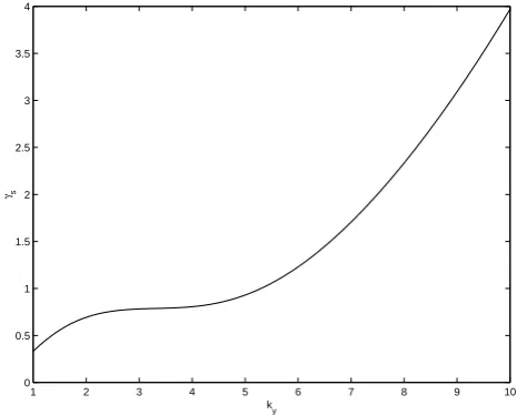
Fig. 1. growth rate for the secondary instability againstky, forkx=
1.0, νin = 0.3, D = 0.2, which indicates that secondary mode
grows in the short scale regime.
new state with finite steady shear flow. In this case, a sta-bility boundary can be determined by settingβ3 = 0. For β3> β1β2, there is a bifurcation with a pair of complex con-jugate roots becoming unstable for Reγs > 0. Figure 1
shows the growth rate for the secondary instabilityγsagainst
ky for the typical values of νin = 0.3 andD = 0.2 and
kx=1.0.
7 Collisional nonlinearity in shear flow generation In the previous analysis of shear flow generation, we have found that the consideration of the mode coupling term shows that the E ×B convection of vorticity (which essentially comes from the ion polarization drift nonlinearity) generates the convective flowsφ0sin(kxx). At the same time, we have
ignored the contribution of the Pedersen drift nonlinearity (∇n·∇φ, which arises due to ion-neutral collision effect) in the flow generation. These two nonlinearities are different in their character, for exampleez×∇φ·∇∇⊥2φ, is normally known as a vector nonlinearity and∇n·∇φis a scalar nonlin-earity; therefore, they contribute differently in the flow gen-eration. For the two modes we have considered, we have seen thatez×∇φ·∇∇⊥2φgenerates an anti-symmetric flow in the
flow profile and similarly, we can see that∇n·∇φgenerates a symmetric flow profile∼cos(kxx). Therefore, to find out
the role of both of the nonlinearities in the flow generation, we have to incorporate symmetric as well as anti-symmetric flows with different amplitudes. In such a scenario, instead of 6 ODE, we have to solve 7 ODE system for the amplitude evolution:
dbφ0
dt = −bφ1bφ2− νinkxk1
ky b
n0bφ
0−νinbφ0, (49) dbφ1
dt = ky
k1bn1+bφ0bφ2− 3 2
νink1kx
ky(3k2x+ky2)
0 5 10 15 20 25 30 35 40 45 50 0.4
0.2 0 0.2 0.4 0.6 0.8 1
time t
φ1
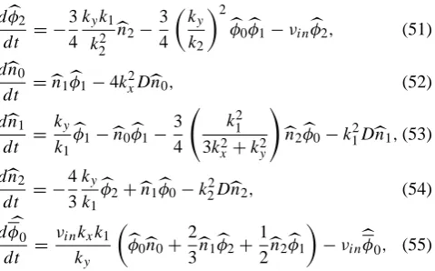
Fig. 2. Potential fluctuation amplitudeφ1, of the fundamental mode forkx =0.4,ky=1.4,νin =0.24 andD=0.2, which indicates
that long scale radial RT mode saturates in time.
dbφ2 dt = −
3 4
kyk1 k22 bn2
−3
4 k
y
k2 2
b
φ0bφ1−νinbφ2, (51) dbn0
dt =bn1bφ1−4k 2
xDbn0, (52) dbn1
dt = ky
k1bφ1−bn0bφ1− 3 4
k12 3k2
x+k2y
!
bn2bφ0−k 2
1Dbn1,(53) dbn2
dt = − 4 3
ky
k1 b
φ2+bn1bφ0−k 2
2Dbn2, (54)
dφb 0 dt =
νinkxk1
ky
b φ0bn0+
2 3bn1bφ2+
1 2bn2bφ1
−νinbφ 0, (55) whereφ0has the same scaling asφ0. Note that the amplitude evolution equation forφ0 (Eq. 55) arises because we have added the symmetric flow termφ0cos(kxx)in our potential
representation.
We must mention that due to the presence of collisional nonlinearity mentioned above, the system no longer supports invariants; therefore, it is practically impossible to analyze 7 ODE system analytically. We have solved Eqs. (49)–(55) numerically using a standard ODE solver routine in MAT-LAB. The initial conditions are taken asn1, φ0, φ0 = 0.1 andn0, n2, φ1, φ2 = 0. The nonzero initial values φ0, φ0 implies that we have initialized the system with a seed shear flow to study their evolutions. The results are shown in the Figs. 2–4 for typical parameters.
We have seen from Eq. (55) that the symmetric shear flow is solely driven by collisional nonlinearity; therefore, in ab-sence of ion-neutral collision, no spatially symmetric shear flow will develop (νin = 0, φ0 = 0). For largeνin(∼ 1),
one might expect that symmetric shear flow will be large, but numerical results show that for largeνin, both symmetric
and anti-symmetric flow decays. Even for moderate values of νin(∼ 0.5)numerical result shows the symmetric shear
flow amplitude is lower than antisymmetric flow amplitude.
0 5 10 15 20 25 30 35 40 45 50
0.4 0.3 0.2 0.1 0 0.1 0.2 0.3 0.4 0.5
time t
φ0a
Fig. 3. Temporal evolution of the anti-symmetric shear flow am-plitude forkx = 0.4,ky = 1.4,νin = 0.24 andD =0.2, which
indicates that the initial seed flow has transient growth and then os-cillatory decay due to finite dissipation present in the system.
Perhaps for a higherνinand finiteD,nφnonlinearity for
var-ious modes decays faster than theφ1φ2nonlinearity; there-fore, the collisional driving term for the flow is weaker than the convective driving term. Thus, even in the collisional regime, the Pedersen nonlinearity may not play a significant role in the shear flow generation and one can justify the ne-glecting of the contribution from the symmetric flow in the analytical calculation in Sect. 4.
8 Discussion and conclusion
0 5 10 15 20 25 30 35 40 45 50 0
0.01 0.02 0.03 0.04 0.05 0.06 0.07 0.08 0.09 0.1
time t φ0s
Fig. 4. Temporal evolution of the symmetric shear flow amplitude forkx =0.4,ky=1.4,νin =0.24 andD=0.2, which indicates
that the initial seed flow does not have significant growth.
the power transfer. The dominant transfer takes place only through the interaction betweenφ1andφ2. The second and higher order effects or other modes influencing the ampli-tude of φ1 and φ2 and thereby contributing to the magni-tude of shear flow generated is also negligible, as the domi-nant change in the amplitude ofφ1comes through the linear growth of the RT mode.
We have done a model calculation to show that due to free energy generated in the quasi-steady bubbles, they are un-stable to secondary instabilities. The mode coupling equa-tions contain a Lorenz attractor on a sub-manifold. Taking the Lorenz branch as a fixed point, we find the dynamical evolution of the remaining three variables in the 6-D phase space. We have shown that nonlinearly formed convective cells or bubbles are unstable to secondary instabilities due to the strong gradient developed by them which trends to frag-ment them into short scales (smaller than the convective cell size). The resulting size of the short scale structure is not cal-culated, since it involves the initial amplitude and nonlinear development of the secondary instabilities. One of the basic mechanism of the onset of turbulence is the destruction of coherent structures and it may be that the secondary instabil-ity mechanism is one of such processes which destroys the structures.
We have not addressed the question of total transport of en-ergy in this study. Most of our discussion, in fact, is involved with a model calculation to illustrate the basic physical fact. To pin down these facts more quantitatively, more investi-gation is needed, for example for the secondary instability, one must consider a 2-D bubble structure as an equilibrium and then perturb it with short scale perturbations in more sys-tematic way. Such a calculation might give us the saturation length scale of such an instability and help us to calculate the transport coefficients. However, from the model calcula-tion, we expect that only moderate scale bubbles can survive,
since large-scale bubbles are ruled out due to secondary in-stability. All of these conclusions are qualitative. In the fu-ture, we hope to address this problem more quantitatively by numerical simulation to clarify some of these issues.
Acknowledgements. Thanks are due to B. P. Pandey and A. K. Sinha
for some helpful discussions.
References
Amatucci, W. E., Walker, D. N., Ganguli, G., et al., Plasma response to strongly sheared flow, Phys. Rev. Lett., 77, 1978, 1996; and reference therein.
Arons, J. and Lea, S. M., Accretion on to magnetized neutron stars: structure and interchange instability of a model magnetosphere, Astrophys. J., 207, 914, 1976.
Basu, B., Generalized Rayleigh-Taylor instability in the presence of time dependent equilibrium, J. Geophys. Res., 102, 17305, 1997. Beyer, P. and Spatschek, K. H., Center manifold theory for the
dy-namics of L-H transition, Phys. Plasmas, 3, 995, 1996.
Burlaga, L. F., Intermittent turbulence in the solar wind, J. Geophys. Res., 96, 5847, 1991.
Chaturvedi, P. K. and Ossakow, S. L., Non-linear theory of the col-lisional Rayleigh-Taylor instability in equatorial spread F ,Geo-phys. Res. Lett., 4, 558, 1977.
Das, A., et al., Nonlinear saturation of Rayleigh-Taylor instability, Phys. Plasmas, 4, 1018, 1997.
Finn, J. M., Nonlinear interaction of Rayleigh-Taylor and shear in-stabilities, Phys. Fluids B, 5, 415, 1993.
Finn, J. M., Drake, J. F., and Guzdar, P. N., Instability of fluid vor-tices and generation of shear flow, Phys. Fluids B, 4, 2758, 1992. Flaherty, J. P., Seyler, C. E., and Trefethen, L. N., Large amplitude transient growth in the linear evolution of equatorial spread F with a sheared zonal flow, J. Geophys. Res., 104, 6843, 1999. Guzdar, P. N., Satyanarayana, P., Huba, J. D., and Ossakow, S. L.,
Influence of velocity shear on Rayleigh-Taylor instability, Geo-phys. Res. Letts., 9, 547, 1982.
Hassam, A. B., Hall, W., Huba, J. D., and Keskinen, M. J., Spectral characteristics of interchange turbulence, J. Geophys. Res., 91, 13513, 1986.
Hassam, A. B., Nonlinear stabilization of the Rayleigh-Taylor in-stability by external velocity shear, Physics Fluids, 4, 485, 1992. Hermiz, K. B., Guzdar, P. N., and Finn, J. M., Improved low or-der model for shear flow driven by Rayleigh-Benard convection, Phys. Rev. E, 51, 325, 1995.
Horton, W., Hu, G., and Laval, G., Trubulent transport in mix states of convective cells and shear flows, Phys. Plasmas, 3, 2912, 1996.
Howard, L. N. and Krshanamurti, R., large scale-flow in turbulent convection: a mathematical model, J. Fluid Mech., 170, 385, 1986.
Huba, J. D., Hassam, A. B., Schwartz, I. B., and Keskinen, M. J., Ionospheric turbulence: Interchange instabilities and chaotic fluid behavior, Geophys. Res. Lett.,12, 65, 1985.
Huba, J. D., Bernhardt, P. A., Ossakaw, S. L., and Zaselak, S. T., The Rayleigh-Taylor instability is not damped by recombination in the F region, J. Geophys. Res., 101, 24553, 1996.
Huba, J. D, Finite larmor radius magnetohydrodynamics of the Rayleigh-Taylor instability, Phys. Plasmas, 3, 2523, 1996. Keskinen, M. J., Sudan, R. N., and Ferch, R. L., Temporal and
gradient drift irregularities in the equatorial electrojet, J. Geo-phys. Res., 84, 1419, 1979.
Lorenz, E. N., Deterministic nonperiodic flow, J. Atmos. Sci., 20, 130, 1963.
Penano, J. R., Ganguli, G., Amatucci, W. E., et al., Velocity shear driven instabilities in a rotating plasma layer, Phys. Plasmas, 5, 4377, 1998.
Pogutse, O., et al., The resistive interchange convection in the edge of tokamak plasma, Plasma Phys. Control Fusion, 36, 1963, 1994.
Satyanarayana, P., Lee, Y. C., and Huba, J. D., Phys. Fluids, 30, 81, 1987.
Sazonov, S. V., Dissipative structures in the F-region of the
equa-torial ionsphere generated by Rayleigh-Taylor instability, Planet. Space Sci., 39, 1667, 1991.
Sudan, R. N. and Keskinen, M. J., Unified theory of power spectrum of intermidiate wavelength ionospheric electron density fluctua-tions, J. Geophys. Res., 89, 9840, 1984.
Volponi, F., Yoshida, Z., and Tatsuno, T., Shear flow induced stabi-lization of kinklike modes, Phys. Plasmas, 7, 2314, 2000. Wilcock, W. S. D. and Whitehead, J. A., The Rayleigh-Taylor
in-stability of an embedded layer of low viscosity fluid, J. Geophys. Res., 96, 12193, 1991.