www.atmos-meas-tech.net/10/955/2017/ doi:10.5194/amt-10-955-2017
© Author(s) 2017. CC Attribution 3.0 License.
Investigating differences in DOAS retrieval codes using
MAD-CAT campaign data
Enno Peters1, Gaia Pinardi2, André Seyler1, Andreas Richter1, Folkard Wittrock1, Tim Bösch1,
Michel Van Roozendael2, François Hendrick2, Theano Drosoglou3, Alkiviadis F. Bais3, Yugo Kanaya4, Xiaoyi Zhao5, Kimberly Strong5, Johannes Lampel6,11, Rainer Volkamer7,8, Theodore Koenig7,8, Ivan Ortega7,8,a, Olga Puentedura9, Mónica Navarro-Comas9, Laura Gómez9, Margarita Yela González9, Ankie Piters10, Julia Remmers11, Yang Wang11, Thomas Wagner11, Shanshan Wang12,13, Alfonso Saiz-Lopez12, David García-Nieto12, Carlos A. Cuevas12,
Nuria Benavent12, Richard Querel14, Paul Johnston14, Oleg Postylyakov15, Alexander Borovski15,
Alexander Elokhov15, Ilya Bruchkouski16, Haoran Liu17, Cheng Liu17,18,19, Qianqian Hong19, Claudia Rivera20, Michel Grutter21, Wolfgang Stremme21, M. Fahim Khokhar22, Junaid Khayyam22, and John P. Burrows1 1Institute of Environmental Physics, University of Bremen, Bremen, Germany
2Royal Belgian Institute for Space Aeronomy (BIRA-IASB), Brussels, Belgium 3Aristotle University of Thessaloniki, Thessaloniki, Greece
4Japan Agency for Marine-Earth Science and Technology (JAMSTEC), Yokohama, Japan 5Department of Physics, University of Toronto, Ontario, Canada
6Institute of Environmental Physics, University of Heidelberg, Heidelberg, Germany 7Department of Chemistry and Biochemistry, University of Colorado, Boulder, CO, USA
8Cooperative Institute for Research in Environmental Sciences (CIRES), University of Colorado, Boulder, CO, USA 9National Institute for Aerospace technology, INTA, Madrid, Spain
10Royal Netherlands Meteorological Institute (KNMI), De Bilt, the Netherlands 11Max Planck Institute for Chemistry, Mainz, Germany
12Department of Atmospheric Chemistry and Climate, Institute of Physical Chemistry Rocasolano, CSIC, Madrid, Spain 13Shanghai Key Laboratory of Atmospheric Particle Pollution and Prevention (LAP3), Department of
Environmental Science & Engineering, Fudan University, Shanghai, China
14National Institute of Water and Atmospheric Research (NIWA), Lauder, New Zealand
15A. M. Obukhov Institute of Atmospheric Physics, Russian Academy of Sciences, Moscow, Russia
16National Ozone Monitoring Research and Education Center BSU (NOMREC BSU), Belarusian State University (BSU),
Minsk, Belarus
17School of Earth and Space Sciences, University of Science and Technology of China, Hefei, 230026, China 18CAS Center for Excellence in Regional Atmospheric Environment, Xiamen, 361021, China
19Key Lab of Environmental Optics & Technology, Anhui Institute of Optics and Fine Mechanics,
Chinese Academy of Sciences, Hefei, 230031, China
20Facultad de Química, Universidad Nacional Autónoma de México, Mexico City, Mexico
21Centro de Ciencias de la Atmósfera, Universidad Nacional Autónoma de México, Mexico City, Mexico 22Institute of Environmental Sciences and Engineering (IESE), National University of Sciences and Technology
(NUST) Islamabad, Islamabad, Pakistan
anow at: National Center for Atmospheric Research (NCAR), Boulder, CO, USA Correspondence to:Enno Peters ([email protected]) Received: 28 October 2016 – Discussion started: 11 November 2016
Abstract. The differential optical absorption spectroscopy (DOAS) method is a well-known remote sensing technique that is nowadays widely used for measurements of atmo-spheric trace gases, creating the need for harmonization and characterization efforts. In this study, an intercomparison ex-ercise of DOAS retrieval codes from 17 international groups is presented, focusing on NO2slant columns. The study is
based on data collected by one instrument during the Multi-Axis DOAS Comparison campaign for Aerosols and Trace gases (MAD-CAT) in Mainz, Germany, in summer 2013. As data from the same instrument are used by all groups, the re-sults are free of biases due to instrumental differences, which is in contrast to previous intercomparison exercises.
While in general an excellent correlation of NO2 slant
columns between groups of>99.98 % (noon reference fits) and>99.2 % (sequential reference fits) for all elevation an-gles is found, differences between individual retrievals are as large as 8 % for NO2slant columns and 100 % for rms
resid-uals in small elevation angles above the horizon.
Comprehensive sensitivity studies revealed that absolute slant column differences result predominantly from the choice of the reference spectrum while relative differences originate from the numerical approach for solving the DOAS equation as well as the treatment of the slit function. Fur-thermore, differences in the implementation of the intensity offset correction were found to produce disagreements for measurements close to sunrise (8–10 % for NO2, 80 % for
rms residual). The largest effect of≈8 % difference in NO2
was found to arise from the reference treatment; in particu-lar for fits using a sequential reference. In terms of rms fit residual, the reference treatment has only a minor impact. In contrast, the wavelength calibration as well as the intensity offset correction were found to have the largest impact (up to 80 %) on rms residual while having only a minor impact on retrieved NO2slant columns.
1 Introduction
In this study, the consistency of differential optical absorp-tion spectroscopy (DOAS) retrievals of tropospheric nitro-gen dioxide (NO2) from ground-based scattered light
obser-vations is evaluated. NO2 is released into the atmosphere
predominantly in the form of NO as a result of combus-tion processes at high temperatures. Through reaccombus-tion of NO with ozone (O3), NO2 is rapidly produced and
(dur-ing the day) back-converted into NO by photolysis. There-fore, nitrogen oxides are often discussed in terms of NOx (NO+NO2=NOx). NO2is a key species in the formation
of tropospheric ozone and a prominent pollutant in the tropo-sphere, causing (together with aerosols) the typical brownish colour of polluted air. In addition, it is harmful for lung tissue and a powerful oxidant. In the lower troposphere, the lifetime of NO2is short (several hours) due to reaction with OH and
photodissociation; thus it is mostly found close to its sources, making it a good tracer of local pollution. Anthropogenic sources such as burning fossil fuel in industry, power gen-eration and traffic as well as biogenic sources including bush and forest fires contribute to the tropospheric NOx loading. In addition, NO2 is released from soil microbial processes
and lightning events (Lee et al., 1997). As a result, high NO2
amounts are mostly observed above industrialized and urban areas, traffic routes and over bush fires.
Using its characteristic absorption bands in the UV and visible spectral range, NO2has been successfully measured
for many years using the DOAS technique (Brewer, 1973; Noxon, 1975; Platt, 1994), both from the ground and from space (e.g. Richter et al., 2005; Beirle et al., 2011). In addi-tion, airborne and car-based measurements (e.g. Schönhardt et al., 2015; Shaiganfar et al., 2011), have been taken to close the gap between ground-based observations providing continuous temporal, but poor spatial resolution and satel-lite measurements which offer global observations, but only up to one measurement per day above each location. Us-ing ground-based multi-axis (MAX)-DOAS measurements at different elevation angles, a more accurate vertical column (VC) can be retrieved with information on the vertical distri-bution of NO2and other trace gases in the troposphere (e.g.
Hönninger et al., 2004; Wittrock, 2006; Frieß et al., 2011; Wagner et al., 2011).
As result of the viewing geometry, ground-based MAX-DOAS observations are most sensitive to the lowest layers of the troposphere. Here they provide high sensitivity and low relative measurement errors. Averaging over longer in-tegration times can further reduce statistical noise. Another advantage is that MAX-DOAS stations can be operated au-tomatically and usually require little maintenance. MAX-DOAS measurements were therefore taken in remote regions for the investigation of background concentrations and in many locations for the validation of satellite observations (e.g. Takashima et al., 2012; Peters et al., 2012).
Figure 1.NO2slant columns and fit residual root mean square (rms) obtained from the IUPB retrieval code for the intercomparison day used in this study. Different elevation angles are colour coded. The fit settings correspond to v1 settings as described in Sect. 2.4 (Table 1).
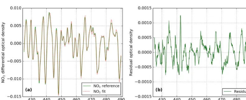
Figure 2. (a)Example of the fitted NO2differential optical density in 2◦elevation angle at 14:40 UT corresponding to a slant column of ≈7E16 molec cm−2(compare Fig. 1). The solid line is the NO2differential optical density (=differential cross section, i.e. the cross section after subtraction of a fitted polynomial, multiplied by the retrieved slant column) and the dashed line is the solid line plus the fit residual. The NO2differential optical density is much larger than the residual, which is explicitly shown in(b).
was the first to also have a focus on MAX-DOAS obser-vations of tropospheric species (Roscoe et al., 2010; Piters et al., 2012; Pinardi et al., 2013) and has recently been fol-lowed by the CINDI-2 campaign carried out in 2016, also in Cabauw. However, these intercomparison exercises concen-trated mostly on results originating from different retrieval codes and instruments, and separation of instrument and re-trieval effects was not easily possible. In some cases, syn-thetic spectra were used to intercompare retrieval algorithms, and while such tests can highlight differences between re-trieval approaches, they give no insight into the way different retrieval codes deal with instrumental effects such as inten-sity offsets, resolution changes or spectral drifts.
The present study was carried out in the framework of the European FP7 project QA4ECV (Quality Assurance for Es-sential Climate Variables), which aims at providing quality assurance for satellite-derived ECVs such as NO2, HCHO
and CO by characterizing the uncertainty budgets through uncertainty analysis and error propagation but also by vali-dation with external data sets. In this context, ground-based MAX-DOAS measurements can play an important role, and harmonization of the retrieval approaches and quality assur-ance for the reference measurements are needed. The results of the analysis in the QA4ECV project are expected to con-tribute to the harmonization of data from MAX-DOAS in-struments, in particular for the ongoing integration of such measurements in the NDACC network.
the Multi-Axis DOAS Comparison campaign for Aerosols and Trace gases (MAD-CAT) carried out in Mainz, Ger-many, in summer 2013 (http://joseba.mpch-mainz.mpg.de/ mad_cat.htm). Data were distributed to 17 international groups working on ground-based DOAS applications. Each group analysed these spectra using their own DOAS retrieval code but prescribed fit settings for fitting window, cross sections, polynomial and offset correction. Resulting slant columns from all groups were then compared to IUPB re-sults chosen as the arbitrary reference, evaluating the level of agreement and systematic differences and investigating their algorithmic origins. With this set-up, nearly all sources of disagreement were removed, and only those differences be-tween retrieval codes were investigated, which are not usu-ally reported.
This intercomparison exercise concentrates on 1 day (18 June 2013) of the MAD-CAT campaign, which had the best weather and viewing conditions. As an example, Fig. 1 shows NO2slant columns (left) and fit rms residual (right) retrieved
with the IUPB software. It can clearly be seen that NO2slant
columns measured at different elevation angles are separated as a result of differences in the light path. It should be men-tioned that NO2slant columns are relatively large as a result
of anthropogenic pollution at the densely populated and in-dustrialized measurement location and thus the findings of this study correspond to polluted urban environments. How-ever, these are normally the ones of interest for NO2
obser-vations. Figure 1 also shows that the rms of the fit residuals (in the following simply denoted rms) separates with eleva-tion angles as well. In addieleva-tion, the shape of the rms in small elevation angles is very similar to that of NO2slant columns,
indicating that predominantly NO2-related effects such as the
wavelength dependence of the NO2AMF (which was not
in-cluded in the fit shown here) limit the fit quality (note that this study aims not at finding best NO2fit settings but
study-ing disagreements originatstudy-ing from different retrieval codes). This is supported by the observation that the shape of NO2
slant columns is not seen in the rms for larger elevation an-gles as effects related to the NO2absorption are smaller and
other effects limiting the fit quality dominate. In addition, the rms is very large in the early morning for small elevations, which is discussed in detail later, and was found to result from pointing towards sunrise. However, in general NO2is
retrieved very accurately as Fig. 2 demonstrates, showing the NO2optical density and fit residual for a measurement in 2◦
elevation angle (this is a typical example fit).
The paper is structured in the following way: Sect. 2 provides details about the MAD-CAT campaign, measure-ments and the NO2intercomparison exercise as well as
par-ticipating retrieval codes. Intercomparison results between groups are presented in Sect. 3. Sensitivity studies of non-harmonized retrieval aspects are described in Sect. 4, at-tempting to reproduce observed differences between groups and evaluating the impact on NO2slant columns and DOAS
fit quality. The paper ends with conclusions and
recom-mendations for better harmonization of ground-based MAX-DOAS measurements.
2 Measurements 2.1 DOAS technique
The DOAS technique is based on Beer–Lambert law, which describes the attenuation of light passing through a medium. Here, it is applied to measurements of scattered sunlight. The spectral attenuation caused by scattering is smooth in wave-length (e.g.λ−4-dependence for Rayleigh scattering) while molecular absorption often has structured spectra. In DOAS, the total spectral attenuation is therefore split into a high-frequency part consisting of the (high-high-frequency components of) trace gas absorptions and a low-frequency part that ac-counts for elastic scattering, which is described by a low-order polynomial, also compensating for intensity changes, e.g. caused by clouds. In addition, the effect of inelastic tering, which is predominantly due to rotational Raman scat-tering, known as the Ring effect (Shefov, 1959; Grainger and Ring, 1962) is accounted for by a pseudo cross section (e.g. Vountas et al., 1998). Similarly, intensity offsets mostly re-sulting from stray light within the spectrometer are accounted for by pseudo cross sectionsσoff(see Sect. 4.3 for more
de-tails). In total, the optical depthτ is approximated by τ=ln
I 0 I =X i
σi·SCi+σRing·SCRing
+σoff·SCoff+
X
p
apλp+r, (1)
where the first sum is over alliabsorbers having cross sec-tion σi, the polynomial degree isp, and the residual term rcontains the remaining (uncompensated) optical depth. An important quantity used within this study to identify and eval-uate differences between DOAS retrieval codes is the root mean square of the fit residualr(for simplicity denoted rms in the context of this study), which is a measure of the fit quality. In Eq. (1), known as the DOAS equation, all quan-tities with the exception ofapdepend on wavelengthλ. For
tropospheric absorbers, the spectrumI is normally taken at small elevation angles above the horizon where the tropo-spheric light path is large. The reference spectrumI0is
nor-mally a zenith spectrum either at small solar zenith angle (SZA), which is called a noon reference fit in the following, or close in time to the measured spectrumI, in the following called a sequential reference fit.
The DOAS equation is usually an overdetermined problem (τ is measured at more wavelengthsλthan unknowns exist in Eq. 1) and solved by means of a least-squares fit (see also Sect. 4.5), i.e. minimizing the residual term. The resulting fit factors are the polynomial coefficientsapand the so-called
along the effective light paths(for simplicity we use the SC also for the fit coefficients of the Ring and offset spectra):
SCi=
Z
ρids. (2)
Note that this is a simplification as normally an ensemble of different light paths contribute to the measurement. In ex-treme cases, the absorption optical depth can become a non-linear function of the trace gas concentration. However, this is usually only of importance for satellite limb measurements and is discussed in detail, for example, in Pukite and Wagner (2016). A comprehensive discussion of the DOAS technique can be found, for example, in Hönninger et al. (2004); Platt and Stutz (2008).
2.2 The MAD-CAT campaign
The Multi-Axis DOAS Comparison campaign for Aerosols and Trace gases (MAD-CAT) was carried out in Mainz, Ger-many, in summer 2013. During the intensive phase of the campaign (7 June to 6 July 2013), 11 groups deployed MAX-DOAS instruments on the roof of the MAX-Planck Institute for Chemistry at the Mainz University campus. Being lo-cated in the densely populated Rhine-Main region, the obser-vations are dominated by anthropogenic pollution, predom-inantly by NO2 (in the visible). The main azimuthal
view-ing direction was 51◦ (from the north), pointing roughly in the direction of the city of Frankfurt≈30 km away. Series of vertical scans comprising elevation angles of 0, 1, 2, 3, 4, 5, 6, 8, 10 and 30◦ were performed. In each direction, single measurements of varying exposure time depending on illumination were integrated for 20 s (for the IUPB in-strument, other instruments used different integration times). Between vertical scans, multiple zenith measurements were taken (see Fig. 1 for an example of resulting NO2 slant
columns). Detailed information about MAD-CAT can be also found at http://joseba.mpch-mainz.mpg.de/mad_cat.htm and the first campaign data focusing on range-resolved distribu-tions of NO2 measured at different wavelengths were
pub-lished by Ortega et al. (2015). Furthermore, Lampel et al. (2015) demonstrated the presence of vibrational Raman scat-tering on N2 molecules in spectra measured during
MAD-CAT. In addition, publications based on MAD-CAT data are in preparation focusing on HCHO (Pinardi, 2017), HONO (Wang et al., 2016) and CHOCHO (Ortega et al., 2017). 2.3 The IUPB MAX-DOAS instrument
The IUPB MAX-DOAS instrument deployed in Mainz during the MAD-CAT campaign is a two-channel CCD-spectrometer system measuring in the UV and visible. Within this exercise, only data from the visible spectrometer are used as NO2is best retrieved in this spectral range. The
spectrom-eter is an ANDOR Shamrock 303i, covering a spectral range from 399 to 536 nm at a resolution of ≈0.7 nm. The
spec-trometer was actively temperature stabilized to 35◦C. Spec-tra were recorded with a charge-coupled device (CCD) of the ANDOR iDUS 420 type with 1024×255 pixels (26×26 µm each), leading to a spectral sampling of 7–8 pixels nm−1.
Light was collected by a telescope unit mounted on a commercial ENEO VPT-501 pan-tilt head allowing point-ing in any viewpoint-ing direction. Photons enterpoint-ing the telescope through a fused silica window were focused by a lens on an optical fibre bundle. The instrument’s field of view (FOV) was≈1.2◦. The Y-shaped optical fibre bundle (length 20 m) connecting the telescope to both spectrometers consists of 2×38=76 single fibres, minimizing polarization effects. A video camera inside the telescope housing takes snap-shots of every recorded spectrum for scene documentation, and a mercury-cadmium (HgCd) line lamp allows for wave-length calibration measurements. Dark current and slit func-tion measurements are taken every night. The same instru-mental set-up has been used in previous campaigns, e.g. CINDI and TransBrom (Roscoe et al., 2010; Peters et al., 2012).
2.4 Intercomparison exercise
Spectra recorded by the IUPB MAX-DOAS instrument on 18 June 2013 during MAD-CAT were distributed to part-ners. It is worth mentioning that this intercomparison ex-ercise was not restricted to groups participating in MAD-CAT, as common observations were provided. 18 June 2013 was selected as having good viewing and weather conditions. However, temperature stabilization of the IUPB spectrome-ter was problematic due to unusually hot weather which, due to a lack of air conditioning on that day, led to the instrument overheating. As a result, spectral stability was not as good as usual, providing the opportunity to investigate how differ-ent retrieval codes deal with potdiffer-ential spectral shifts during the day. The provided data comprised observations at sev-eral elevation angles in the main azimuthal viewing direc-tion of 51◦(see Fig. 1 for an example). In addition, common trace gas cross sections as well as DOAS fit settings were distributed as summarized in Table 1, which are the com-mon fit settings agreed on during the MAD-CAT campaign. All groups then performed DOAS fits using these prescribed settings on IUPB spectra using their own retrieval software. The influence of different retrievals was then analysed, fo-cusing on the impact on NO2columns. A brief description
of retrieval codes is given in the following. The participat-ing groups (with abbreviations used within this study) and retrieval codes they used are summarized in Table 2. 2.4.1 NLIN
decompo-Table 1.Summary of fit settings used for the NO2intercomparison. These fit settings were agreed on during the MAD-CAT campaign and can be found also at http://joseba.mpch-mainz.mpg.de/mad_analysis.htm.
Fit Reference Window Cross sections Intensity offset Polynomial
v1 noon 425–490 1, 2, 4, 5, 6, 7 constant (0th order) 5 (6 coefs) v1a sequential 425–490 1, 2, 4, 5, 6, 7 constant (0th order) 5 (6 coefs) v2 noon 411–445 1, 3, 4, 5, 6, 7 constant (0th order) 4 (5 coefs) v2a sequential 411–445 1, 3, 4, 5, 6, 7 constant (0th order) 4 (5 coefs)
Cross sections
1 NO2at 298 K (Vandaele et al., 1996),I0-correction using 1×10¹⁷molec cm−2 2 NO2at 220 K orthogonalized to 298 K within 425–490 nm
3 NO2at 220 K orthogonalized to 298 K within 411–445 nm 4 O3at 223 K (Bogumil et al., 2003)
5 O4Hermans et al., unpublished, http://spectrolab.aeronomie.be/o2.htm 6 H2O, HITEMP (Rothman et al., 2010)
7 Ring, NDSC2003 (Chance and Spurr, 1997)
Table 2.Summary of participating institutes (with abbreviation) and retrieval codes used by each group.
Abbr. Retrieval(s) Institute
IUPB NLIN Institute for Environmental Physics, University of Bremen, Germany AUTH QDOAS Aristotle University of Thessaloniki, Greece
BIRA QDOAS Belgian Institute for Space Aeronomy, Brussels, Belgium JAMSTEC QDOAS Japan Agency for Marine-Earth Science and Technology, Japan Toronto QDOAS Department of Physics, University of Toronto, Ontario, Canada IUPHD DOASIS Institute of Environmental Physics, University of Heidelberg, Germany Boulder QDOAS University of Colorado, Boulder, USA
KNMI KMDOAS Royal Netherlands Meteorological Institute, De Bilt, The Netherlands INTA LANA National Institute for Aerospace technology, Madrid, Spain
MPIC MDOAS, Max Planck Institute for Chemistry, Mainz, Germany WinDOAS
CSIC QDOAS Department of Atmospheric Chemistry and Climate,
Institute of Physical Chemistry Rocasolano, CSIC, Madrid, Spain
NIWA STRATO National Institute of Water and Atmospheric Research, Lauder, New Zealand
IAP RS.DOAS A. M. Obukhov Institute of Atmospheric Physics, Russian Academy of Sciences, Moscow, Russia BSU WinDOAS Belarusian State University, Minsk, Belarus
USTC QDOAS University of Science and Technology, Hefei, China UNAM QDOAS National Autonomous University of Mexico, Mexico NUST QDOAS Institute of environmental sciences and engineering (IESE),
National University of Sciences and Technology, Islamabad, Pakistan
sition (SVD) which is comprised in an iterative non-linear fit for calibration of the wavelength axis using a Marquardt– Levenberg fit.
2.4.2 QDOAS
QDOAS (Dankaert et al., 2013) is the multi-platform (Windows, Unix/Linux and Mac) successor of WinDOAS. A coupled linear/non-linear least squares (NLLS) algorithm (Marquardt-Levenberg fitting and SVD decomposition) is used to solve the DOAS equation including a wavelength calibration module. During this operation, the slit function can be characterized in addition to the wavelength
2.4.3 LANA
LANA is a two-step iterative algorithm developed at INTA and used since 1994. In the first step, cross sections and spec-tra are positioned and in the second step the linear equations system is solved using a Gauss–Jordan procedure. For this exercise, the intensity offset correction was based on the ref-erence spectrumI0.
2.4.4 MDOAS
MDOAS is a Matlab DOAS code developed at MPIC, but calibration and convolution have been performed in WinDOAS. For sequential reference fits, two versions, MPIC_MDa and MPIC_MDb, are included in this exercise, which used a different treatment of the Ring spectrum. 2.4.5 KMDOAS
KMDOAS was recently (2013–2014) developed at KNMI and verified using QDOAS. It is written in Python using stan-dard modules (matplotlib, numpy, scipy, pandas).
2.4.6 DOASIS
DOASIS has been used by IUPHD in its version 3.2.4595.39926. A detailed explanation can be found in (Kraus, 2006). In the version submitted here, an additional shift of cross sections with respect to the optical depth was allowed and a saturation correction was implemented. 2.4.7 STRATO
The NIWA-Strato package was originally (1980s) used for processing zenith DOAS spectra, but extended as needed to handle MAX-DOAS measurements. The fitting code uses least squares or optional SVD fitting inside iterations apply-ing shift, stretch and (optional) offset, for minimum resid-ual. In contrast to other groups, an internal equidistant wave-length grid is applied using the average interpixel spacing. 2.4.8 RS.DOAS
RS.DOAS (Ivanov et al., 2012; Borovski et al., 2014; Postylyakov et al., 2014; Postylyakov and Borovski, 2016) was developed by IAP. The DOAS inversion is performed by LU decomposition. The wavelength calibration uses sev-eral subwindows, and for each of them a non-linear shift and stretch fit including all trace gases (resulting from the linear DOAS fit) is applied. From a set of shifts obtained for the subwindows a 2nd-order polynomial approximation of the shift dependency on pixel number is constructed. For con-voluting cross sections the QDOAS software (offline version 2.0 at 5 March 2012) was used.
2.4.9 WinDOAS
WinDOAS (Fayt and Van Roozendael, 2001) is the precursor of QDOAS. It has been used by BSU as well as MPIC for this intercomparison exercise (the MPIC submission is denoted MPIC_WD, the reference has been selected by hand), but only for noon reference fits.
3 Intercomparison results
3.1 Noon reference, 425–490 nm fit window (v1 fit parameters)
Differences between groups for the 425–490 nm fit using a noon reference (v1 fit settings; see Table 1) are shown in Fig. 3 for individual measurements at an elevation angle of 2◦. Small elevation angles above the horizon are associated with long tropospheric light paths and are therefore impor-tant for the detection of tropospheric absorbers. Differences shown in Fig. 3 are relative to IUPB results. For the objective of identifying retrieval-code-specific effects, the use of a sin-gle retrieval code as a reference seems advantageous in com-parison to using the mean of all retrieval codes which would average over all retrieval-specific features. Note that this does not exclude IUPB from the intercomparison as problems with the IUPB retrieval would be easily detected, leading to the same systematic patterns in all lines shown in Fig. 3.
Absolute differences (institute-IUPB) and relative differ-ences (absolute difference/IUPB) of NO2slant columns and
fit rms are shown in Fig. 3a–d. In general, NO2slant column
differences are in the range of±2–3×10¹⁵molec cm−2 or
<2 %. This is about a factor of 2–3 larger than NO2 slant
column errors, which are typically<1×10¹⁵molec cm−2or <0.6 % for 2◦ elevation. A clearly enhanced disagreement is observed for the first data point in the INTA time series as well as for MPIC_WD. The latter could be linked to the reference spectrum, which in this case is not the one with the smallest sun zenith angle (SZA), while the outlier in the INTA time series was identified to arise from different imple-mentations of the intensity offset correction (see Sect. 4.3). Note that these NO2differences for individual measurements
are much smaller than the variability (diurnal cycle) of NO2
and thus almost invisible in Fig. 3e where no differences but absolute NO2 slant columns from each groups
(includ-ing IUPB in black) are plotted.
Interestingly, many groups show a smooth behaviour (con-stant offset) in absolute NO2differences (Fig. 3a), which is
mostly an effect of the choice of the reference (see Sect. 4.1), while relative differences (Fig. 3c) reflect the shape of NO2
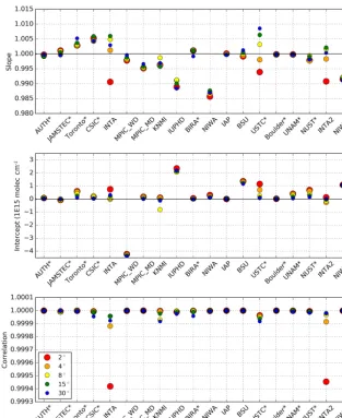
Figure 4.Linear regression results (slope, intercept, correlation) for different elevation angles (with respect to IUPB) for fit settings v1 (noon reference). Groups using QDOAS (in different versions) are indicated by a star (∗).
in relative differences. These two types are linked to differ-ences in retrieval codes, which are investigated in detail in Sect. 4.
Absolute rms differences (with respect to IUPB) in Fig. 3b show the same shape as NO2 slant columns. This is
be-cause at small elevations the rms itself reflects the shape of the NO2, which was already demonstrated and discussed in
Fig. 1. A better measure for the identification of differences between retrieval codes is thus the relative rms disagreement shown in Fig. 3d. Interestingly, the first data point for INTA, showing a large disagreement with IUPB and other groups in NO2 slant columns is prominent in absolute rms
differ-ences as well, but not in relative rms differdiffer-ences. The reason is that the rms in the morning is very large (Fig. 3f, compare also to Fig. 1) and thus decreases the relative difference. Re-markably, relative rms differences are found up to 80–100 %, which is substantially more than NO2 slant column
differ-ences (only a few percent).
overheat-ing of the system on this day. In general, time series of shifts shown in Fig. 3g and h agree well in shape. A small off-set is observed for NIWA, who successfully found and cor-rected a fault in their retrieval code (related to the intensity offset calculation) in the course of this exercise. The DOAS fit was then repeated using the corrected retrieval code and the result, called NIWA2, is included in Fig. 3. Apparently, NIWA2 shows a much better comparison than other groups (most obvious in the fitted spectral shift) and performs better because the rms in Fig. 3d is much smaller than before. Sim-ilarly, INTA fixed a problem in their retrieval code related to the wavelength calibration. The reanalysed INTA data are denoted INTA2 in Fig. 3. The INTA2 shift is comparable to other groups, while large disagreements were seen before, and the rms is largely reduced in comparison to the first INTA submission. Notably, almost no differences between INTA and INTA2 are observed in terms of NO2 slant columns;
in particular the first data point is still outlying. This indi-cates (1) that the wavelength calibration has a large impact on the fit rms but only a minor impact on the NO2 slant
columns, and (2) that the disagreement of the first data point is not related to the wavelength calibration. Despite INTA and NIWA, only KNMI is fitting a rather different shift (and provides the shift only in 0.01 nm resolution which leads to the displayed discrete steps). This is caused by different def-initions of the shift (see Sect. 4.6): KNMI is fitting the shift of the optical depth relative to the cross sections while the other groups are fitting the shift ofI relative to the reference spectrumI0. As a result, the shift of KNMI and other groups
cannot be expected to match.
The agreement between groups, including other elevation angles, has been quantified by linear regression analyses to correlation plots (of each group relative to IUPB results, not shown). Resulting slopes, offsets and correlation coefficients are summarized in Fig. 4 and colour-coded for different el-evation angles. As expected, the correlation coefficient is >99.98 % with the only exception of the INTA (and INTA2) 2◦ elevation which is predominantly caused by the outlier already seen in Fig. 3. The slope ranges between 0.985 and 1.01, the offset between−4 and 2.5×10¹⁵molec cm−2. Apart from USTC and INTA, no large separation of the slope and offset with elevation angle is observed. An impor-tant observation is that groups using the same retrieval code (QDOAS) do not necessarily show the same systematic be-haviour in Fig. 4, implying that the influence of remaining fit parameters that are different from the harmonized general settings in Table 1 is still larger than the effect of the spe-cific retrieval software used. For example, the best agreement in terms of slope, offset and correlation coefficient is found between IUPB, AUTH, IAP and CU Boulder, which all use different retrieval codes.
3.2 Other fit parameters
The agreement between groups was investigated in the same way when using a sequential reference (denoted v1a fit set-ting; see Table 1) instead of a noon reference spectrum (v1 fit). A sequential reference is often preferred if tropospheric absorbers are of interest as stratospheric effects are removed to a large extent.
Figure 5 is similar to Fig. 3, but some groups are missing here (e.g. IAP) as they only provided noon reference fits. The range of disagreements for individual NO2slant columns is
up to≈8 % and therefore larger than NO2disagreements
us-ing a noon reference (v1 fit). In addition, neither absolute nor relative differences between groups are smooth (Fig. 5a and c). The reason is that, in contrast to the noon reference, a different (zenith)I0 spectrum is used for every scan and
thus the impact of details of the implementation of the refer-ence changes from scan to scan. Different implementations of the reference spectrum are further investigated in Sect. 4.1 and were found to be the major reason for NO2
disagree-ments between groups. The outlier (first data point) seen for v1 (noon) fit settings is present for v1a as well but it is not prominent here as fluctuations for the above-mentioned rea-son are of same magnitude.
In terms of rms, differences between groups are compara-ble to v1 results and as large as≈80 %.
Compared to the noon reference fit, correlations from lin-ear regressions (not shown) are smaller, especially for the 30◦ elevation angle, mainly resulting from the larger disagree-ments as explained above (but also partly expected as slant columns are smaller using a sequential reference). Correla-tions are still>99.2 % for 30◦elevation and even>99.8 % for smaller elevations.
In addition to the 425–490 nm fit (v1 and v1a), a smaller fit window used within the MAD-CAT campaign was inter-compared (v2 and v2a using a spectral range of 411–445 nm; see Table 1). Results of these fits are not explicitly shown as mainly confirming observations and findings above. Typi-cal correlation coefficients (as well as offsets and slopes) are summarized in Table 3 for all fits. A very small tendency of better agreement between groups if using the larger fit win-dow is seen. Although this should not be overinterpreted, it could be caused by more information being present in the large fit window and therefore more accurate results (fewer statistical fluctuations).
4 Sensitivity studies of non-harmonized retrieval aspects
Figure 5.Results from v1a fit settings (sequential reference spectrum) on 2◦elevation angle data as a function of time.(a, b)Absolute NO2 slant column and rms differences,(c, d)relative NO2slant column and rms differences. All differences are relative to IUPB. Triangular markers indicate groups using QDOAS, circular markers indicate groups using independent software, and diamonds indicate groups that corrected faults in their code during the course of this study and submitted a reanalysed data set.
Table 3.Correlations, slopes and offsets from linear regressions on NO2slant columns between each group and IUPB (neglecting the INTA 2◦outlier).
Fit Correlation Slope Offset
(%) (1×10¹⁵molec cm−2) v1 >99.98 0.985 to 1.01 −4 to 3 v1a >99.2 0.96 to 1.01 −1.5 to 1 v2 >99.94 0.985 to 1.005 −4 to 3 v2a >99.2 0.96 to 1.01 −2 to 1
sources of differences in the DOAS fit results: (1) the se-lection/calculation of the reference spectrum, predominantly for sequential reference fits, (2) treatment of the slit function, (3) the intensity offset correction, (4) differences in the nu-merical calculation of the DOAS fit (linear fit) and (5) differ-ences in the wavelength calibration (non-linear fit). In the fol-lowing, tests using the same retrieval code (IUPB) have been performed to characterize the impact of each of the above-mentioned systematic differences.
4.1 Effect of the reference spectrum
In the IUPB spectra provided to intercomparison partners, two different zenith spectra at the same smallest SZA were
reported, which is of course non-physical. Actually, the sec-ond zenith spectrum is the one with the smallest SZA, but for rounding reasons (the SZA was a 4-digit number in the input data provided), both spectra had the same SZA. Con-sequently, for the noon reference fits v1 and v2 within this intercomparison exercise, four options exist: (1) taking the first zenith spectrum of smallest SZA, (2) taking the second one, (3) taking the first for the morning and the second for the afternoon (i.e. always taking the closest in time) and (4) tak-ing the average of both spectra. Similarly, different options exist for calculating the sequential references for fits v1a and v2a: (1) always taking the zenith spectrum closest in time, (2) always taking the last zenith spectrum before the actual measurement, (3) always taking the next zenith spectrum af-ter the measurement, (4) taking the average of the two (before and after) and (5) interpolating the two zenith spectra to the time of the actual measurement.
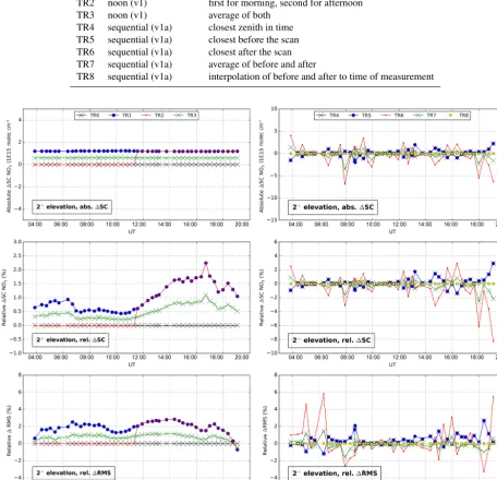
All different options for noon and sequential reference fits were evaluated using the IUPB retrieval code NLIN (Ta-ble 4). Figure 6 shows the resulting absolute and relative slant column differences (top and middle) as well as relative rms differences (bottom) for noon reference (left) and sequential reference (right) with respect to v1 or v1a fit results.
Table 4.Tests performed to study the influence of different reference spectra.
Test Reference (fit setting) Remarks
TR0 noon (v1) first spectrum of smallest SZA TR1 noon (v1) second spectrum of smallest SZA TR2 noon (v1) first for morning, second for afternoon TR3 noon (v1) average of both
TR4 sequential (v1a) closest zenith in time TR5 sequential (v1a) closest before the scan TR6 sequential (v1a) closest after the scan TR7 sequential (v1a) average of before and after
TR8 sequential (v1a) interpolation of before and after to time of measurement
Figure 6.Different test results (see Table 4) in 2◦elevation angle as a function of time. Top panel shows absolute NO2SC differences, middle shows relative SC differences, bottom shows relative rms differences. Left is for noon reference (differences are with respect to IUPB v1 fit results), right is for sequential references (differences are with respect to IUPB v1a fit results).
Test TR0 (using the first spectrum) yields the same results as the IUPB v1 fit from Sect. 3, which uses the first zenith spectrum as well. In contrast, using the second zenith spec-trum as a reference (TR1) results in a constant offset of 1.5×10¹⁵molec cm−2(0.5–2.5 % in relative differences, de-pending on the actual NO2slant column), because the second
zenith spectrum apparently had a smaller NO2content. The
change of the NO2content could be related to changes of the
atmospheric NO2amount or the atmospheric light path. In
terms of rms, TR1 is up to 3 % larger (Fig. 6, bottom left). The main reason for this is probably the larger NO2 slant
depen-dence of the NO2slant column (Pukite et al., 2010) were not
compensated in this intercomparison exercise as discussed in Sect. 1.
Test TR2 yields results which are identical to TR0 am and TR1 pm values. This is not seen for any groups in Fig. 3 above; i.e. this option is apparently not present in any re-trieval code. Not surprisingly, TR3 (averaging both zenith spectra) yields results which are between TR0 and TR2.
In contrast to noon reference tests, sequential references show no smooth behaviour, neither for absolute nor for rel-ative differences (Fig. 6, right). The reason is that for each vertical scanning sequence (from which only the 2◦elevation is shown here and in Fig. 3) another reference spectrum is used and consequently reference-related differences between groups are also changing from scan to scan. Note that almost no difference can be seen in Fig. 6 between TR4 and TR5 as the 2◦ elevation angle is shown here and consequently the closest zenith measurement in time is normally the one before the scan as IUPB measurements proceed from low to large elevations. TR8 (interpolation to the measurement time) resembles the sequential reference treatment normally implemented in the IUPB code; thus the TR8 line is zero. For TR6 and TR7, absolute and relative differences (up to 8 %) are remarkably similar to observed differences between groups using v1a fit settings, both in shape and in absolute values (compare to Fig. 5).
To conclude, the exact treatment of reference spectra is the major reason for observed NO2 discrepancies between
groups in Sect. 3, causing differences of up to 8 %. Unfortu-nately, no clear recommendation can be derived from relative rms differences in Fig. 6 (bottom right) as all lines scatter around zero. However, the relative difference in rms can be as large as 6 % and in general, using a single zenith reference spectrum before or after the scan tends to produce larger rms. However, while the reference treatment explains the majority of NO2disagreements, it cannot explain the large rms
differ-ences (up to 100 %) between groups. 4.2 Slit function treatment
The slit function distributed to intercomparison participants originated from HgCd line lamp measurements made in the night before 18 June 2013. It was preprocessed in terms of subtraction of the (also measured) dark signal, centred and provided on an equidistant 0.1 nm grid.
While some groups used this slit function as is, other re-trieval codes include a further online processing of the slit function, e.g. by fitting line parameters. In order to evaluate resulting differences, trace gas cross sections have been con-volved offline (before the fit) using different treatments of the slit function as summarized in Table 5. Again, the IUPB re-trieval code NLIN has been used then performing the DOAS fit.
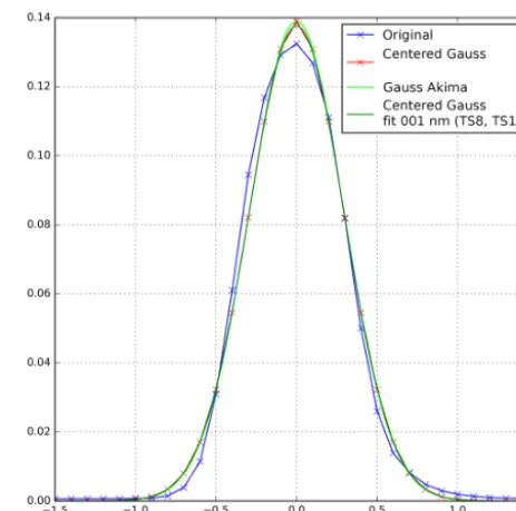
Examples of different treatments of the slit function are shown in Fig. 7. The original slit function is displayed in
Figure 7.Examples of different slit function treatments. Blue is the measured slit function (from HgCd line at≈480 nm). Red is the fit of a Gaussian shape withµ=0. Light green is the Akima interpolation of the red line to a finer 0.01 nm grid. Dark green is the interpolation first (linearly) to 0.01 nm and fit of a Gaussian shape afterwards.
blue. If fitting a Gaussian shape to it, the maximum is not exactly centred around zero, presumably caused by a small asymmetry. The slit function after fitting a Gaussian shape and forcing centring (i.e.µ=0) is shown in red (as used in TS7 and TS10). Furthermore, performing a discrete convo-lution of cross sections requires the same wavelength sam-pling; i.e. the slit function has to be interpolated to the cross section grid, which was 0.01 nm. Here, an Akima interpo-lation has been applied (green line). However, if the origi-nal slit function is first linearly interpolated to the required 0.01 nm grid and then a Gaussian shape is fitted, a slightly different result is obtained, shown in dark green (as used in TS8 and TS11). Note that often not a discrete convolution but a (faster) convolution using Fourier transformation is im-plemented in DOAS retrieval codes (see below).
Figure 8 shows resulting absolute and relative differences in NO2 slant columns (top and middle) as well as relative
differences of the fit rms (bottom) with respect to the IUPB v1 fit (without I0-correction as this was not applied to the slit function test fits). The reference IUPB v1 fit uses an online convolution of cross sections using FFT and a further geo-metrical centring of the slit function is applied.
No difference between the reference fit, TS0 and TS5 is observed, neither for NO2nor for the rms. In TS0, the same
ad-Table 5.Different treatments of the slit function.
Test Sub. offset Geom. centring Cut-off value Fit line parameters
TS0 no yes 0.0 no
TS1 no no 0.001 no
TS2 yes no 0.001 no
TS3 no yes 0.001 no
TS4 yes yes 0.001 no
TS5 no no 0.0 no
TS6 no no 0.001 Gaussian
TS7 no no 0.001 Gaussian (µ=0)
TS8 no no 0.001 Gaussian (µ=0) fitted on 0.01 nm grid
TS9 no no 0.0 Gaussian
TS10 no no 0.0 Gaussian (µ=0)
TS11 no no 0.0 Gaussian (µ=0) fitted on 0.01 nm grid
Figure 8.NO2slant columns and rms differences with respect to IUPB v1 fit results in 2◦elevation angle for different treatments of the slit function.
dition, TS5 and TS0 are identical tests except that TS0 ap-plies an explicit geometrical centring (i.e. centring the area) of the slit function. As this has no visible effect on NO2slant
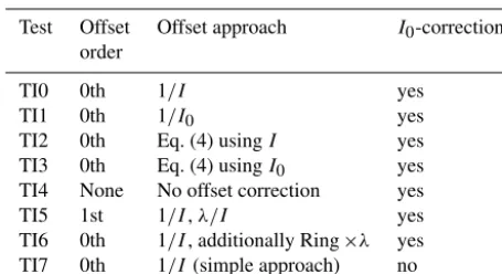
Table 6. Tests performed for different implementations of the in-tensity offset correction (andI0correction). A 0th-order offset cor-rection means applying a constant term only, a 1st-order corcor-rection means applying a constant and slope term.
Test Offset Offset approach I0-correction order
TI0 0th 1/I yes
TI1 0th 1/I0 yes
TI2 0th Eq. (4) usingI yes
TI3 0th Eq. (4) usingI0 yes
TI4 None No offset correction yes
TI5 1st 1/I,λ/I yes
TI6 0th 1/I, additionally Ring×λ yes TI7 0th 1/I(simple approach) no
The largest impact on NO2(up to−1.3 %) is seen for TS2
and TS4 which both subtract the smallest value from the slit function (i.e. forcing the slit function to be zero for the small-est value measured). This is usually not performed in DOAS fits and only advisable if instrumental stray light is a large problem or if the dark signal drifts which is normally not the case in state-of-the-art CCD detectors that are cooled and temperature-stabilized using Peltier elements.
In contrast, the largest effect in terms of rms (up to 6.5 %) occurs not for TS2 and TS4, but for all tests using a fit-ted Gaussian. Interestingly, the Gaussian tests (TS6–TS11) show almost no difference among them in terms of rms in the morning, but split up towards the evening. This might have to do with decreasing NO2slant columns in the afternoon or
changes of the slit function during the day. In terms of NO2,
all tests using Gaussian slit functions yield smaller NO2slant
columns of 0.2–0.7 %.
In addition to the basic Gaussian line parameters fitted here, some retrieval codes offer the possibility of fitting more sophisticated line shape parameters while taking into account potential asymmetry much better (the slit function in Fig. 7 shows indeed slight asymmetry). However, the exact imple-mentations differ and were therefore not reproduced in the tests performed here, which can then be regarded as two extreme scenarios, namely (1) using the (original, slightly asymmetric) slit function as it is, or (2) fitting basic line pa-rameters (a more sophisticated fit taking into account the slit function’s slight asymmetry would clearly lead to a result in between these scenarios).
An important finding is that all performed tests lead to con-stant offsets in relative (and not absolute) NO2differences. In
addition, all tests yield larger rms than the reference fit using the measured slit function.
4.3 Intensity offset correction
Photons may hit the CCD detector at locations not corre-sponding to their wavelength (e.g. through scattering on
mir-rors, surfaces etc. inside the spectrometer) which produces an intensity offset, also called stray light. In addition, other effects such as changes in the dark current can lead to in-tensity offsets and the vibrational Raman scattering (VRS) is known to produce spectral effects that are very similar to intensity offsets (Peters et al., 2014; Lampel et al., 2015). In the DOAS fit, pseudo cross sections are usually included in order to compensate for intensity offsets. If the measured spectrumIis superimposed by a constant intensityC(which is the most simple assumption), the optical depth reads
−τ =ln I+C
I0 =ln I I0 +ln
1+C
I ≈ln I I0 +C
I, (3)
with the Taylor expansion ln(1+x)≈x. Thus, in a first ap-proximation the intensity offset causes an additive term of optical depth that is proportional to 1/I, which is often used as a pseudo absorber (and showing large similarities to the Ring cross section as this compensates a filling-in of Fraun-hofer lines).
However, often more sophisticated approaches are used. For example, the IUPB retrieval code NLIN allows either the simple implementation ofσoff=1/I or
σoff=ln
I+C·I
max
I
, (4)
omitting the Taylor expansion in Eq. (3) and superimposing I by a certain constantC of the maximum intensity within the fit interval. In addition, higher correction terms are also sometimes used, assuming that, not only does a constant su-perimposes the spectrum, but a contribution also changes with wavelength (in which case oftenλ/I is included in the DOAS fit). Furthermore, sometimes the offset is not included in the linear DOAS fit, but fitted non-linearly (this is not in-cluded in tests performed here).
Different implementations summarized in Table 6 were tested in order to evaluate the influence of the intensity off-set correction. Figure 9 shows resulting absolute and relative differences of NO2slant columns and rms values. Again, the
reference for these differences is the IUPB v1 (noon) fit. No difference in NO2or rms is seen between TI0 and the
v1 fit as both fits use the same simple approach ofσoff=1/I.
In contrast, TI1 uses 1/I0. In terms of NO2differences, the
TI1 line slightly follows the shape of total fit rms and NO2
slant columns (compare to Fig. 3). Interestingly, while the disagreement of TI1 with respect to the reference fit is on average≈2 % for NO2, the first data point is clearly off by
almost 10 % for NO2and 60 % for rms. This agrees perfectly
Figure 9.Absolute (top) and relative (middle) NO2slant column differences and relative rms differences (bottom) with respect to IUPB v1 fit results in 2◦elevation angle resulting from different implementations of the intensity offset correction (andI0correction).
of this measurement are ≈90 and 58◦(from the north), re-spectively, while the instrument’s elevation angle is 2◦and the azimuthal viewing direction 51◦; i.e. the instrument was pointing close to the rising sun. Enhanced stray light in the spectrometer (caused by the large contribution of photons at longer wavelengths while observing the red sky during sun-rise) seems plausible and using 1/I is a better choice for compensation. It was verified (not shown) that the fit coef-ficient of the offset (also called the offset slant column) is particularly large not only in this but also in adjacent mea-surements and a colour index indicated that these spectra are indeed more reddish. However, these measurements could also be affected by direct sunlight in the instrument, which is known to increase rms (e.g. due to polarization issues). Figure 3f demonstrates that the respective measurement is affected by a very large rms (potentially caused by a combi-nation of direct light and stray light).
TI2 and TI3 are more sophisticated approaches (Eq. 4) based on eitherI orI0. However, the resulting lines largely
follow TI0 and TI1 (simple approaches). Unexpectedly, both TI2 and TI3 lead to larger rms values for the sunrise mea-surement in the morning where the simple approach performs better.
The total effect of using an intensity offset compensation is evaluated by TI4 which includes no offset correction. The resulting effect on NO2is almost the same as TI1 and TI3
(based onI0) leading to the clear recommendation of using
an offset compensation based onI instead of I0, which is
supported by largely increased rms values of TI4 (Fig. 9 bot-tom).
An intensity offset correction of 1st-order (i.e. a term vary-ing linearly withλin addition to a constant term) was tested in TI5, which is in practice often used not only for inten-sity offsets but also for compensation of the wavelength-dependence of the Ring slant column. The resulting NO2
morning. Interestingly, the TI5 rms line shows some similar-ities to the IUPHD-IUPB line in Fig. 3d. However, no 1st-order offset was included in the IUPHD fit; i.e. the offset im-plementation is not causing the observed similar shape in the morning (and the reason remains unclear). This is supported by increasing IUPHD rms values in the evening in Fig. 3d, which are not present in TI5.
Fit TI6 includes again only a 0th-order intensity offset, but a pseudo cross section accounting for the wavelength-dependence of the Ring slant column was added (the Ring cross section was multiplied byλand orthogonalized against the original cross section). The resulting rms is indeed al-most identical to TI5 (using a 1st-order intensity offset) while the NO2is identical to TI0; i.e. the outlying first data point
which is still partially present in TI5 disappeared in TI6. Thus, using a pseudo-cross section for compensation of the Ring wavelength-dependence seems preferable compared to using a 1st-order intensity offset correction.
4.4 I0-correction
In addition to the intensity offset tests, the effect of inclusion of anI0-correction was evaluated in TI7 (which is identical to
TI0 except for theI0-correction; see Table 6). The respective
line is shown in addition to the intensity offset investigations in Fig. 9. TheI0-effect addresses the problem that the limited
instrument’s resolution can cause an incomplete removal of Fraunhofer structures in the vicinity of strong narrow-banded absorption bands (Johnston, 1996; Wagner et al., 2001; Ali-well et al., 2002).
Only a very small constant offset in relative NO2 slant
column differences is obtained in TI7 (≈0.25 %, which is almost invisible in Fig. 9, middle). In terms of rms, exclu-sion of the I0-correction leads to an increased rms of up to
20 %, which is comparable to different treatments of the in-tensity offset correction. Thus, including anI0-correction is
recommended in polluted environments such as the MAD-CAT site. It should be noted that the first data point is not an outlier in TI7; i.e. it is not sensitive to theI0-correction.
4.5 Numerical methods (linear DOAS inversion) The DOAS equation (Eq. 1) is a linear inverse problem
Ax=b, (5)
with the vector x (size n) containing the ntrace gas slant columns and polynomial coefficients of interest, the vector b=ln(I0
I)(size m) containing the measured optical depths at mwavelengths and them×nDOAS matrixAwith columns consisting of absorption cross sections and polynomial terms (1,λ,λ2, etc.) for themwavelengths.
Different numerical methods exist to solve Eq. (5) forx. As A is non-square, no inverse exists. However, most re-trieval codes calculate a pseudo-inverse A−1 (almost) ful-fillingA−1A=I(identity matrix) using a singular value
de-composition (SVD) and obtain the slant columns of interest byx=A−1b. This method is frequently recommended for
solving overdetermined linear inverse problems in terms of least squares (see e.g. Press, 1989).
However, after multiplying Eq. (5) with AT, the matrix ATAis quadratic and can be decomposed into an upper and a lower triangular matrix,LandU. The linear inverse problem
ATAx=LUx=ATb (6)
can then be solved by a forward substitution, obtaining y fromL y=ATb, and a backward substitution, obtainingx fromUx=y.
Furthermore,ATAcan also be directly inverted, normally by LU decomposition as well. The vector of slant columns is then obtained byx=(ATA)−1ATb. As the inversion nor-mally takes many more computational steps, this method is known to be subject to round-off errors and is therefore not recommended (Press, 1989).
The influence of these different numerical methods on re-sulting slant columns could not be easily tested with the IUPB retrieval code and was thus evaluated in a Python script solving the DOAS equation using the same input (spec-tra, cross sections). Python (which is a well-established pro-gramming language in scientific computing) provides numer-ous different routines within its numpy and scipy packages (based on different subroutines from the LAPACK package, http://www.netlib.org/lapack/) that were tested for solving the DOAS equation. All performed tests are summarized in Table 7. Again, differences of NO2slant columns and fit rms
have been calculated with respect to the IUPB v1 fit results (i.e. using NLIN). In order to restrict differences to the in-fluence of numerical approaches only, the same slit function treatment as the IUPB retrieval code NLIN was applied in the Python script and the same (noon) reference spectrum was used. In addition, no further wavelength calibration, i.e. no non-linear shift and squeeze fit, was performed (neither in the Python script nor in the NLIN reference fit used here) and noI0-correction was included. The test results are shown in
Fig. 10, again for the 2◦elevation angle.
Results of test TL0 appear to be identical to the reference fit of the IUPB retrieval code, both using a SVD for inver-sion of the DOAS matrix. However, very small differences exist between TL0 and the reference fits (too small to be seen on the scale of Fig. 10), which are<0.006 % for NO2slant
columns and<0.07 % for rms. These tiny disagreements can be attributed to numerical differences in programming lan-guages.
TL1 and TL2 yield identical NO2slant columns (both are
Table 7.Different methods tested for solving the linear DOAS equationAx=b.
Test Retrieval Spectral Method Remarks
code grid
Reference NLIN I0 Pseudo-inverse ofAusing SVD following Press (1989) TL0 Python I0 Pseudo-inverse ofAusing SVD
TL1 Python I0 Solving quadraticATAx=ATb using LU decomposition TL2 Python I0 InvertATAusing LU decomp.
and multiply withATb
TL3 Python 0.01 nm same as TL0 linear interpolation
to 0.01 nm
TL4 Python 0.01 nm same as TL0 cubic spline interpolation
to 0.01 nm
are differences with respect to IUPB) are similar in shape to the total fit rms (compare to Fig. 3f). Thus, when the rms in-creases, SVD inversion and LU decomposition lead to larger disagreements, both in rms and NO2. As the SVD yields
smaller rms values, it seems to be preferable, although the obtained improvement is only about 2.5 %.
Numerical differences may be obtained when perform-ing the linear DOAS fit (Eq. 5) on another wavelength grid. Changes of the grid potentially arise from the wavelength calibration. Some retrieval codes (e.g. NIWA) also use an internal, equidistant wavelength grid. To test the effect of changes in the wavelength grid, the TL0 fit was repeated on an equidistant 0.01 nm grid (i.e.I,I0and cross sections were
interpolated to 0.01 nm before solving Eq. 5). TL3 and TL4 are identical to TL0, but a linear interpolation was applied in TL3, while TL4 uses a cubic spline interpolation to 0.01 nm. Apparently, this results in a constant offset in relative NO2
differences, which is seen most clearly in the TL3 line in Fig. 10 (middle). The resulting constant shift is≈0.4 % for TL3, but only≈0.02 % for TL4 meaning that the type of in-terpolation to the equidistant grid is of importance and the spline interpolation (not surprisingly) seems to resemble the spectrum better than a linear interpolation. However, using different wavelength grids might, for example, explain some of the observed differences between IUPB and NIWA, which were found to be constant in relative differences as well. In terms of rms, the computation on an equidistant 0.01 nm grid using linear interpolation behaves even a bit better on aver-age (up to 1 %). However, no recommendation can be drawn from this, as discussed above.
4.6 Non-linear wavelength calibration
As mentioned in Sect. 2.3, the spectra provided from the IUPB instrument were precalibrated using nightly HgCd line lamp measurements, which provide accuracies better than 0.1 nm. However, usually a postcalibration is included in DOAS retrieval codes in order to increase the fit qual-ity (reducing rms). This wavelength calibration is
imple-mented in different ways in participating retrieval codes. Most groups calibrate the reference spectrumI0 to a
high-resolution Fraunhofer atlas, apply the resulting calibration to all measured spectra and allow in addition a shift and squeeze betweenI andI0 in order to compensate spectral shifts of
the spectrometer during the day, e.g. caused by temperature changes (KNMI uses a slightly different definition of the shift as discussed below). This non-linear shift and squeeze fit of the wavelength axis is mostly implemented in an iterative scheme together with the linear DOAS fit on ln(I0/I ).
How-ever, codes differ, for example in whether trace gases are in-cluded in the shift and squeeze fit ofI0to the high-resolution
Fraunhofer atlas. Sometimes also a higher-order calibration is allowed or several subwindows are used in order to differ-ently characterize different parts of the spectra.
Table 8 summarizes tests performed to investigate the im-pact of different wavelength calibration approaches using the IUPB retrieval code NLIN. In addition, some tests were per-formed with the Python script form Sect. 4.5, which has therefore been extended to perform the non-linear shift fit as not all tests could be easily implemented in the com-prehensive NLIN software. Note that, in contrast to the shift, the squeeze has been excluded from the intercompar-ison as it was found to always be 1.0 for measurements shown here. Also, QDOAS-specific implementations were not tested here.
Figure 11 shows the resulting impact on NO2 and rms
as well as the fitted shift betweenI andI0(not present in
all tests). NO2and rms are again differences relative to the
IUPB v1 fit results (withoutI0-correction as this was not
im-plemented in the Python routine). As in Fig. 3, the shift in Fig. 11d is no difference, and for comparison the shift from the reference fit is shown explicitly in black. The (fixed) shift retrieved from the non-linear fit ofI0to the Fraunhofer atlas
is−0.035 nm. This is roughly a factor of 10 larger than the fitted shift betweenIandI0shown in Fig. 11d. It is
Figure 10.Absolute (top) and relative (middle) NO2slant column differences and relative rms differences (bottom) with respect to IUPB v1 results (only linear fit) in 2◦elevation angle resulting from different numerical methods solving the linear DOAS equation.
Table 8.Different wavelength calibration approaches evaluated.
Test Retrieval code ShiftI0to Shift Remarks code Fraunhofer atlas ItoI0
Reference NLIN_D yes yes alternating scheme, v1 fit settings
TW0 NLIN_D no no linear DOAS fit only
TW1 NLIN_D no yes
TW2 NLIN_D yes no
TW3 Python yes yes same a TW0
TW4 Python yes yes same a TW3, but linear interpolation
TW5 Python yes yes same a TW3, all trace gases
included in FraunhoferI0fit
and also indicating the presence of the tilt effect (Lampel et al., 2017).
The most extreme test is TW0, which excludes both the calibration of I0to the Fraunhofer atlas as well as the shift
betweenI andI0. When omitting both calibration steps, the
Figure 11.Absolute(a)and relative(b)NO2slant columns differences and relative rms differences(c)in 2◦elevation angle resulting from different wavelength calibration approaches (Table 8). Corresponding shifts betweenIandI0resulting from non-linear fits are shown in(d).
registration module was corrected) in Fig. 3d. Although all of these groups are performing a wavelength calibration, TW0 indicates that differences in the calibration procedure are causing most of the disagreements between groups in terms of rms. This is in contrast to NO2 where changes of only
0.4 % are obtained from TW0.
TW1 still excludes the absolute calibration to the Fraun-hofer atlas, but includes the shift fit between I andI0. As
seen before, the impact on NO2is very small (≈0.4 %), but
absolute NO2 differences of TW1 reflect the shape of
to-tal rms and NO2slant columns (compare to Fig. 3); i.e. the
relative differences are smooth in shape. The rms is simi-lar in shape to TW0, but the morning maximum is slightly later at 07:00 UT; the noon maximum is around 11:00 UT and a small maximum in the evening occurs at 18:00 UT. This shape is similar to the relative rms of NUST, UNAM and NIWA in Fig. 3, but the absolute numbers are differ-ent. However, this behaviour indicates that differences in the fitted Fraunhofer shift are partially responsible for observed differences between these and other groups. Interestingly, the fitted shift betweenIandI0of TW1 in Fig. 11d is very
sim-ilar to corresponding values of the reference fit, which is be-cause the missing Fraunhofer shift is a different effect than the shift betweenI andI0.
In contrast to TW1, TW2 includes the Fraunhofer shift fit, but excludes the shift betweenI andI0. As this is the larger
effect (−0.035 nm compared to only≈0.004 nm), the rms is much smaller than in TW1 with a single maximum (up to 50 %) in the early morning at 06:00 UT. The rms time se-ries shape is similar to the KNMI line in Fig. 3. The reason
is a different definition of the shift in the KNMI retrieval: while in most retrievalsIis shifted relative toI0, KNMI
cal-culates the optical depthτ=ln(I0/I )without any shifts but
then allows a shift of all cross sections relative toτ. This is in first order compensating the effect of the Fraunhofer shift but neglecting potential shifts betweenI andI0(in this case
Fraunhofer lines would not cancel out completely in the op-tical depthτ). As a result, the KNMI approach is similar (but not identical) to TW2. The fit quality following the KNMI approach is expected to be better using a sequential reference as the temperature drift of the spectrometer is much smaller then. It has to be mentioned that the change of NO2in TW2
is small (0.3 %) compared to the change in fit rms (50 %). TW3 uses the same wavelength calibration treatment as the IUPB reference fit, but was run in another programming code (Python) to evaluate how much difference is caused by use of another programming code and numerical issues. The fitted shift is mostly identical to the reference fit except for the early morning and late evening when the NO2also shows
very slight differences. The largest disagreement of NO2is
0.2 % for the first measurement of the day that was affected by large stray light effects (and potentially direct light) and thus most likely indicating cross-correlations between shift fit and intensity offset correction. The resulting rms is almost identical to the reference fit (Fig. 11c).
TW4 is the same as TW3 but the spline interpolation (cal-culatingI at spectral points ofI0during the non-linear shift
fit) is replaced by a simple linear interpolation. The fitted shift is changed slightly and NO2differences are of almost
Table 9.Summary of performed sensitivity tests and associated impacts on NO2slant columns and rms.
Reason for disagreement 1NO2( %) 1rms ( %) Remarks
Reference treatment (noon) 2.5 3 Produces constant absolute NO2SC offsets. Reference treatment (seq.) 8 6
Slit function treatment 1.3 6.5 Produces constant relative NO2SC offsets. Intensity offset correction 2 (typically) 20 (typically)
10 (outlier) 60 (outlier)
I0correction 0.25 20 Produces constant relative NO2SC offsets. Numerical methods 0.3 (0.7) 2.5 Produces constant relative NO2SC offsets.
(for linear DOAS fit) Disagreements increase with rms.
Wavelength calibration 0.4 up to 80 (non-linear shift fit)
demonstrating that the shift fit has a negligible impact on NO2. In contrast, it has a large impact on rms, where the
marginally different methods between TW3 and TW4 pro-duce the same rms while the effect of excluding the shift completely leads to largely enhanced rms.
In the Fraunhofer calibration of the reference fit using NLIN (non-linear shift fit ofI0) as well as in TW3 all trace
gas absorptions are omitted; i.e. an iterative scheme between shift fit and DOAS fit comprising only a polynomial of or-der 4 is applied. In contrast, all trace gas absorptions are included in the Fraunhofer calibration in TW5. As a result, the rms of the DOAS fit between the Fraunhofer spectrum andI0is reduced by a factor of 2 and the non-linearly
fit-ted shift is−0.031 nm instead of−0.035 nm in the reference fit. However, this only has a marginal influence on NO2, rms
and fitted shift betweenIandI0in Fig. 11 and consequently
explains none of the observed differences between groups. Notably, all shifts (even TW1) in Fig. 11d show the same general shapes that are retrieved by most groups in Fig. 3. Only shifts of KNMI clearly differ, for the reasons mentioned above. Rms shapes in Fig. 11c suggest that differences in the wavelength calibration are the major reason for observed rms disagreements between groups in Fig. 3.
5 Summary and conclusions
An intercomparison of DOAS retrieval codes using measured spectra from the same instrument during the MAD-CAT campaign and harmonized fit settings was performed. Excel-lent agreement was found between different DOAS fit algo-rithms from 17 international groups. In some of the retrieval codes, faults were identified and corrected in the course of the study, leading to even better agreements. For noon refer-ence fits, the correlation in terms of NO2slant columns was
found to be larger (>99.98 %) than for sequential references (>99.2 %), which is caused by different implementations of the sequential reference.
Despite the excellent overall correlation, for individual measurements in low elevations differences of up to 8 % in
resulting NO2slant columns were observed, which is up to
2–3 times larger than corresponding typical NO2 slant
col-umn errors. In terms of fit rms, large differences of up to
≈100 % were found.
Interestingly, groups using the same retrieval code (QDOAS groups) do not always produce results showing the same systematic behaviour, which is the result of dif-ferent options users select – other than the harmonization settings agreed on. This has some impact for the interpreta-tion of other studies as the extent of prescribed fit settings in this study is comparable to intercomparison campaigns like CINDI or CINDI-2. Consequently, groups participating in those campaigns will provide intrinsic differences in their results due to non-harmonized (detailed) settings even if us-ing the same retrieval code, which has to be expected in the same range as observed here.
Comprehensive sensitivity studies systematically investi-gating effects of the non-harmonized retrieval aspects were performed in order to (1) attribute observed differences be-tween groups to certain sources and (2) evaluate the impact of each of these sources on NO2slant columns and fit rms.
For this purpose, five causes were identified in a survey of participating retrieval codes. Typical impacts on NO2 slant
columns and rms are summarized in Table 9.
In general, the wavelength calibration and the intensity offset correction were found to produce the majority of ob-served rms differences, but have a negligible impact on NO2
slant columns (<0.4 % or <2 % except for the first mea-surement of the day affected by stray light and possibly di-rect light in the telescope). In contrast, the reference selection explains the majority of observed NO2slant column
differ-ences between groups while having a minor impact on the rms. Thus, if harmonization of NO2slant columns is of