www.nonlin-processes-geophys.net/22/133/2015/ doi:10.5194/npg-22-133-2015
© Author(s) 2015. CC Attribution 3.0 License.
Time-dependent Long’s equation
M. Humi
Department of Mathematical Sciences, Worcester Polytechnic Institute, 100 Institute Road, Worcester, MA01609, USA Correspondence to: M. Humi ([email protected])
Received: 15 October 2014 – Published in Nonlin. Processes Geophys. Discuss.: 10 November 2014 Revised: 21 January 2015 – Accepted: 8 February 2015 – Published: 6 March 2015
Abstract. Long’s equation describes steady-state two-dimensional stratified flow over terrain. Its numerical so-lutions under various approximations were investigated by many authors. Special attention was paid to the properties of the gravity waves that are predicted to be generated as a re-sult. In this paper we derive a time-dependent generalization of this equation and investigate analytically its solutions un-der some simplifications. These results might be useful in the experimental analysis of gravity waves over topography and their impact on atmospheric modeling.
1 Introduction
Long’s equation (Long, 1953, 1954, 1955, 1959) models the flow of inviscid stratified fluid in two dimensions over ter-rain. When the base state of the flow (that is, the unper-turbed flow field far upstream) is without shear the solutions of this equation are in the form of steady lee waves. Solu-tions of this equation in various settings and approximaSolu-tions were studied by many authors (Drazin, 1961; Drazin and Moore, 1967; Durran, 1992; Lily and Klemp, 1979; Peltier and Clark, 1983; Smith, 1980, 1989; Yih, 1967). The most common approximation in these studies was to set the Brunt– Väisälä frequency to a constant or a step function over the computational domain. Moreover, the values of the parame-tersβ andµwhich appear in this equation were set to zero. In this (singular) limit of the equation the nonlinear terms and one of the leading second-order derivatives in the equa-tion drop out and the equaequa-tion reduces to that of a linear harmonic oscillator over two-dimensional domain. Careful studies (Lily and Klemp, 1979) showed that these approxi-mations are justified unless wave breaking is present in the solution (Peltier and Clark, 1983; Miglietta and Rotunno, 2014).
Long’s equation provides also the theoretical framework for the analysis of experimental data (Fritts and Alexander, 2003; Shutts et al., 1988; Vernin et al., 2007; Jumper et al., 2004) under the assumption of shearless base flow. (An as-sumption which, in general, is not supported by the data.) An extensive list of references appears in Fritts and Alexan-der (2003), Baines (1995), Nappo (2012) and Yhi (1980).
An analytic approach to the study of this equation and its solutions was initiated recently by the current author (Humi, 2004). We showed that for a base flow without shear and un-der rather mild restrictions the nonlinear terms in the equa-tion can be simplified. We also identified the “slow vari-able” that controls the nonlinear oscillations in this equation and using phase averaging approximation derived a formula for the attenuation of the stream function perturbation with height. This result is generically related to the presence of the nonlinear terms in Long’s equation. We explored also differ-ent formulations of this equation (Humi, 2007, 2009) and the effect of shear on the solutions of this equation (Humi 2006, 2010).
applica-tion to atmospheric modeling (Richter et al., 2010; Geller et al., 2013).
The plan of the paper is as follows: in Sect. 2 we derive the time-dependent Long’s equation. In Sect. 3 we consider the time evolution and proper boundary conditions on shearless flow over topography. We end with the summary and conclu-sion in Sect. 4.
2 Derivation of the time-dependent Long’s equation
In the paper we consider the flow in two dimensions (x,z) of an inviscid, stratified and weakly compressible fluid that is modeled by the following equations:
ux+wz=0, (1)
ρt+uρx+wρz=0, (2)
ρ (ut+uux+wuz)= −px, (3)
ρ (wt+uwx+wwz)= −pz−ρg, (4)
where subscripts indicate differentiation with respect to the indicated variable, u=(u, w) is the fluid velocity, ρ is its density,pis the pressure andgis the acceleration of gravity. One possible interpretation of Eq. (1), is that the fluid is incompressible while Eq. (2) is an advection equation for a scalar (viz.ρ) by the flow. However, since we consider, in the following, derivatives of the density we refer to this formula-tion as representing a “weakly compressible fluid”.
We can nondimensionalize these equations by introducing x= x
L, z= N0
U0
z, u= u
U0
, w=LN0
U02 w,
¯
ρ= ρ
ρ0
, p= N0
gU0ρ0
p, (5)
where L, U0, and ρ0 represent respectively characteristic
length, velocity, and density.N0is the characteristic Brunt–
Väisälä frequency: N02= −g
ρ dρ
dz, (6)
whereρis the ambient density profile of the atmosphere. In the following we letN0to be a constant.
In these new variables Eqs. (1)–(4) take the following form (for brevity we drop the bars):
ux+wz=0, (7)
ρt+uρx+wρz=0, (8)
βρ (ut+uux+wuz)= −pz, (9)
βρ (wt+uwx+wwz)= −µ−2(pz+ρ) , (10)
where β=N0U0
g , (11)
µ= U0
N0L
. (12)
β is the Boussinesq parameter (Shutts et al., 1988; Baines, 1995) which controls stratification effects (assumingU06=0)
andµis the long wave parameter which controls dispersive effects (or the deviation from the hydrostatic approximation). In the limitµ=0 the hydrostatic approximation is fully satis-fied (Baines, 1995; Nappo, 2012). It should be observed that these two parametersβ andµencapsulate the atmospheric conditions which impact the creation of gravity waves over terrain although one of them (µ) can be suppressed by addi-tional scaling.
In view of Eq. (7) we can introduce a stream functionψ so that
u=ψz, w= −ψx. (13)
Using this stream function we can rewrite Eq. (8) as ρt+J{ρ, ψ} =0, (14)
where for any two (smooth) functionsf,g, J{f, g} =∂f
∂x ∂g ∂z−
∂f ∂z
∂g
∂x. (15)
Usingψ the momentum equation Eq.( 9), Eq. (10) be-comes
βρ (ψzt+ψzψzx−ψxψzz)= −px, (16)
βµ2ρ (−ψxt−ψzψxx+ψxψxz)= −pz−ρ. (17)
We can suppressµfrom the system (Eqs. 14, 16, 17) if we introduce the following normalized independent variables: t= t
µ, x= x
µ, z=z, µ6=0. (18) Equations (14) and (16) remain unchanged and Eq. (17) be-comes
βρ (−ψxt−ψzψxx+ψxψxz)= −pz−ρ, (19)
where we dropped the bars ont,x, andz. However, we ob-serve that in these coordinatesψz=uandψx= −µ w.
Thus, after all these transformations the system of equa-tions governing the flow is Eqs. (14), (16) and (19).
To eliminate p from Eqs. (16) and (18) we differentiate these equations with respect tozandxrespectively and sub-tract. This leads to
βρz(ψzt+ψzψzx−ψxψzz)
+βρ (ψzzt+ψzψzzx−ψxψzzz)
−βρx(−ψxt−ψzψxx+ψxψxz)
−βρ (−ψxxt−ψzψxxx+ψxψxxz)=ρx. (20)
The sum of the second and fourth terms in this equation can be rewritten as
βρh∇2ψt+J n
(However, observe that when µ6=1, ∇2ψ does not repre-sent the flow vorticity due to the transformation Eq. (18) and therefore the sum of the two terms in Eq. (21) is not zero in general.)
To reduce the first and third terms in Eq. (20) we use Eq. (14). We obtain
β
ρz(ψzt+ψzψzx−ψxψzz)
−β
ρx(−ψxt−ψzψxx)+ψxψxz
=βρzψzt+ρzψzψzx−(ρt+ρxψz) ψzz
+ρxψxt+(ψxρz−ρt) ψxx−ρxψxψxz
=β
ρzψzt+ρxψxt−ρt∇2ψ+
1 2 Jn(ψx)2+(ψz)2, ρ
oo
. (22)
Combining the results of Eqs. (21) and (22), Eq. (20) be-comes
ρ h
∇2ψ
t
+J
n
∇2ψ, ψ oi
+ρzψzt+ρxψxt
+
−ρt∇2ψ+
1 2J
n
(ψx)2+(ψz)2, ρ o
=J{ρ, z}
β . (23) Thus, we have reduced the original four equations (Eqs. 1–4) to two equations (Eqs. 14 and 23). This system of equations can be considered as the generalization of Long’s equation to time-dependent flows.
While Eq. (23) is rather complicated in general it can be simplified further in some special cases. The first is when one considers the steady state of the flow. (This simplifies also Eq. 14.) This restriction leads to Long’s equation (Long, 1953, 1954, 1955, 1959; Baines, 1995; Yhi, 1980). Further-more, if the density derivatives associated with the momen-tum terms are neglected Eq. (23) reduces to the 2-D Boussi-nesq equation (Tabaei et al.,2005). Another case happens when∇2ψ=0; i.e.,ψis harmonic. (Note, however, that this does not imply that the physical vorticity∇ ×uis zero due to the transformation Eq. (18) unlessµ=1.) Equation (23) becomes
ρzψzt+ρxψxt+
1 2J
n
(ψx)2+(ψz)2, ρ o
=J{ρ, z}
β . (24) Observe that the derivatives ofρwith respect to time are not present in this equation and this is consistent with Eq. (1).
However, if ∇2ψ=0 we can define v1=ψz and
v2= −ψx. These definitions use the stretched coordinates of
Eq. (18) and then (v1)z−(v2)x=0.
This implies that there exists a functionηso that ηx=v1, ηz=v2.
That is,
ηx=ψz, ηz= −ψx.
Physically, these relations imply thatηx=uandηz=µ w.
Replacingψbyηin Eq. (24) yields J
ηt+
1 2 h
(ηx)2+(ηz)2 i
+ z
β, ρ
=0. (25)
Hence, ηt+
1 2 h
(ηx)2+(ηz)2 i
+z
β =R(ρ), (26) whereR(ρ)is a parameter function that can be determined from the asymptotic conditions on the flow. This equation is formally similar to the Bernoulli equation withηplaying the role of the velocity potential. Whenµ=1 and the term βz is interpreted as potential energy,ηrepresents potential flow.
To summarize, the equations of the flow in this case are ρt+ηxρx+ηzρz=0 (27)
(which replaces Eq. 14), and Eq. (26). 2.1 Other reductions of Eq. (23)
The reduction of Eq. (23) was carried out above under the assumption∇2ψ=0. However, it can be generalized to case
∇2ψ=a, whereais a constant. To this end we define v1=ψz, v2= −ψx+ax.
Therefore, (v1)z−(v2)x=0,
which implies that there exists a functionηso that ηx=v1, ηz=v2.
Hence,
ηx=ψz, ηz= −ψx+ax. (28)
Using these relations to substituteηforψin Eq. (23) leads to
ρzηxt−ρx(ηz−ax)t
+
−aρt+
1 2J
n
(ηz−ax)2+(ηx)2, ρ o
=J{ρ, z}
β . (29)
Therefore,
J{ηt, ρ} −aρt+
1 2J
n
(ηz−ax)2+(ηx)2, ρ o
=J{ρ, z}
β . (30)
Hence,
−aρt+J
ηt+
1 2 h
(ηz−ax)2+(ηx)2 i
+z
β, ρ
=0. (31)
−aJ{ψ, ρ} +J
ηt+1
2 h
(ηz−ax)2+(ηx)2 i
+z β, ρ
=0. (32)
It follows then that
−aψ+ηt+
1 2 h
(ηz−ax)2+(ηx)2 i
+z
β =R(ρ). (33) We can eliminate ψ from this equation by differentiating with respect tozand use Eq. (28):
−aηx+
ηt+
1 2 h
(ηz−ax)2+(ηx)2 i
z
= −1
β+R(ρ)z. (34)
3 Time evolution of stratified flow
In this section we shall consider the time evolution of a stratified shearless base flow, viz. a flow which satisfies as t→ −∞,
limx→−∞ρ0(t, x, z)=
H−z
H ,limx→−∞u=1,limx→−∞v=0; (35)
i.e., the far upstream flow is independent of time and satisfies asymptoticallyu=1,v=0, andρ0is stratified with height (H is a height at which ρ0≈0). The conditions onu and v imply that asymptoticallyη0=x. We note that this is the standard setup that has been used to analyze experimental observations of gravity waves (Jumper et al., 2004; Vernin et al., 2007; Shutts et al., 1988). The solutions of Eqs. (26) and (27) which we discuss below represent therefore gravity waves which are generated by low lying topography.
In these limits Eq. (27) is satisfied. Substituting these lim-iting values in Eq. (26) we obtain that
R(ρ)= z
β + 1 2=
H (1−ρ) β +
1
2. (36)
However, it is obvious that different profiles of the base flow will yield a differentR(ρ).
We now consider perturbations from the (shearless) base flow described by Eq. (35) due to shape of the topography, viz.
η=η0+φ, ρ=ρ0+ζ. (37) From Eqs. (26) and (27) we obtain to first-order inthe fol-lowing equations forφandζ:
∂φ ∂t +
∂φ ∂x +
H ζ
β =0, (38)
∂ζ ∂t +
∂ζ ∂x−
1 H
∂φ
∂z =0. (39)
To find the general form of the solution of these equations we use Eq. (38) to expressζ in terms ofφand substitute in Eq. (39). This yields the following equation forφ:
−100 −5 0 5 10 15 20 25 30 0.02
0.04 0.06 0.08 0.1 0.12 0.14 0.16
x
ζ
t=0 t=2*pi t=4*pi t=6*pi t=8*pi
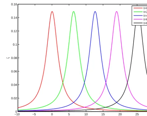
Figure 1. A cross section of the perturbation inρatz=2.
∂2φ ∂t2 +2
∂2φ ∂t ∂x+
∂2φ ∂x2+
1 β
∂φ
∂z =0. (40) It is possible to find “elementary solutions” to this equation by separation of variables if we let
φ=p(t, x)F (z),
wherecis an arbitrary positive constant so thatφrepresents a perturbation moving forward in time. This leads to
∂2p ∂t2 +2
∂2p ∂t ∂x+
∂2p ∂x2
p = −
1 β
F (z)0 F (z) = −ω
2, (41)
whereω2is the separation of variables constant. Primes de-note differentiation with respect to the appropriate variable.
Solving Eq. (41) we obtain the following elementary solu-tion forφ:
φω=Cωexp h
βω2zi[G(x−t )cosωt+K(x−t )sinωt], (42) whereG(x−t),K(x−t) are arbitrary smooth functions and Cωis a constant.
The corresponding solution forζ can be obtained by sub-stituting this result in Eq. (38):
ζ=Cω βω
H exp
h
βω2zi[G(x−t )cosωt−K(x−t )sinωt]. (43) Hence, the general solution forφcan be written as
φ= ∞ Z
0
exphβω2zi[Gω(x−t )cosωt+Kω(x−t )sinωt] dω (44)
0 10 20 30 40 50 60 70 80 90 100 −0.4
−0.3 −0.2 −0.1 0 0.1 0.2 0.3 0.4 0.5
t
ζ
z=0 z=1.6 z−3.2 z=4.9 z=6.5
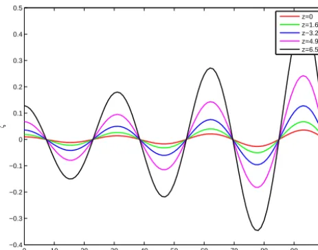
Figure 2. A cross section of the perturbation inρatx=20.
3.1 Boundary conditions
We consider a flow in an unbounded domain over topogra-phy with shape f (x) and maximum height h and impose the following boundary conditions onρandψ in the limits x= −∞andt= −∞:
ψ (−∞,−∞, z)=z, ρ(−∞,−∞, z)=ρ0(z). (45) (This implies that in these limitsη=x.)
At the topography we impose the following boundary con-dition onρatt=0:
ρ(0, x, f (x))=ρ0(f (x))=H−f (x)
H (46)
but
ρ(0, x, f (x))≈ρ0(0, x,0)+ζ (0, x, z). Hence, at the topography
ζ (0, x, f (x))= −f (x)
H . (47)
To derive the corresponding boundary condition for η we first consider the appropriate boundary condition on the stream function ψ along the topography. To this end we assume that the topography is a line on which the stream function is constant and this constant can be chosen to be zero. For the base flow described in Eq. (45), ψ0=z and
ψ=ψ0+ ψ1whereψ1is the perturbation due to to the
to-pography. Hence, along the topography 0=ψ0+ψ1=z+ψ1(0, x, f (x))
=f (x)+ψ1(0, x, f (x)). (48)
Therefore, along the topography we let ψ1(0, x,
f (x))= −f (x). We now observe that by definition
ψx=ηz. But ψx= ψx1= − f0(x), (where primes denote
differentiation with respect tox) andη= −x+ φ. There-fore, we infer that the boundary condition on η along the topography is
φz(0, x, f (x))= −f0(x) (49)
(which is consistent with Eq. 39).
As to the boundary condition onη(t,∞,z), we observe that the system of Eq. (26) and Eq. (27) contains no dissi-pation terms and therefore only radiation boundary condi-tions can be imposed in this limit. (Physically, this means that the horizontal group velocity is positive and energy is radiated outward.) Similarly, atz= ∞it is customary to im-pose (following Peltier and Clark, 1983) radiation boundary conditions. However, in view of Eqs. (42) and (43) it is ob-vious that the perturbation described by these equations is propagating forward in time and this condition is satisfied. A formal verification of this constraint is possible by express-ingF,G, andKin these equations using Fourier transform representation.
For low lying topography (viz1) it is customary to replace the boundary conditions Eqs. (46) and (47) by ζ (0, x,0)= −f (x)
H , φz(0, x,0)= −f 0
(x). (50) Example: iff (x)is given by a “witch of Agnesi” curve, then
f (x)= a
2
a2+x2, f 0
(x)= − 2a
2x
x2+a22. (51) Let the initial perturbation inρbe
ζ (0, x, z)=eβλ2z,
whereλis a constant. From Eq. (50) we infer that the general expression forζ is given by Eq. (43) withω=λ. Hence, at t=0 we must have
G(x)= −f (x)
βλ .
Similarly, the boundary condition onφyields
K(x)= −f
0(x)
βλ2 .
Figures 1 and 2 exhibit cross sections of the perturbation at z=2 andx=20 at different times withCω=0.1,a=2, and
4 Summary and conclusions
Steady-state solutions of Long’s equation model the verti-cal structure of plane parallel gravity waves. These solu-tions are useful, for example, in the parameterizasolu-tions of unresolved gravity wave drag where the WKBJ (Wentzel– Kramers–Brillouin–Jeffreys) approximation is invoked to de-scribe the time-dependent amplitude spectrum of a packet of gravity waves propagating in a slowly varying background.
The present paper presents an alternative analytical approach to solve (under several restrictions) this and similar time-dependent problems without having to invoke the WKBJ approximation. The analytical insights derived from this approach might be used to complement and verify the numerical results obtained from the WKBJ method.
Acknowledgements. The author is indebted to the the anonymous
referees whose comments helped improve the quality of this paper.
Edited by: V. I. Vlasenko
Reviewed by: Two anonymous referees
References
Baines, P. G.: Topographic effects in Stratified flows. Cambridge Univ. Press, New York, 1995.
Drazin, P. G.: On the steady flow of a fluid of variable density past an obstacle, Tellus, 13, 239–251, 1961.
Drazin, P. G. and Moore, D. W.: Steady two dimensional flow of fluid of variable density over an obstacle, J. Fluid. Mech., 28, 353–370, 1967.
Durran, D. R.: Two-Layer solutions to Long’s equation for verti-cally propagating mountain waves, Q. J. Roy. Meteorol. Soc., 118, 415–433, 1992.
Fritts, D. C. and Alexander, M. J.: Gravity wave dynamics and effects in the middle atmosphere, Rev. Geophys., 41, 1003, doi:10.1029/2001RG000106, 2003.
Geller, M. A., Alexander, M. J., Love, P. T., Bacmeister, J., Ern, M., Hertzog, A., Manzini, E., Preusse, P., Sato, K., Scaife, A. A., and Zhou, T.: A comparison between gravity wave momentum fluxes in observations and climate models, J. Climate, 26, 6383–6405, 2013.
Humi M : On the Solution of Long’s Equation Over Terrain, Il Nuovo Cimento C, 27, 219–229, 2004.
Humi M : On the Solutions of Long’s Equation with Shear SIAM J. Appl. Math., 66, 1839–1852, 2006.
Humi, M.: Density representation of Long’s equation, Nonlin. Pro-cesses Geophys., 14, 273–283, doi:10.5194/npg-14-273-2007, 2007.
Humi, M.: Long’s equation in terrain following coordinates, Non-lin. Processes Geophys., 16, 533–541, doi:10.5194/npg-16-533-2009, 2009.
Humi, M.: The effect of shear on the generation of gravity waves, Nonlin. Processes Geophys., 17, 201–210, doi:10.5194/npg-17-201-2010, 2010.
Jumper, G. Y., Murphy, E. A., Ratkowski, A. J., and Vernin, J.: Mul-tisensor Campaign to correlate atmospheric optical turbulence to gravity waves, AIAA paper AIAA-2004-1077, 42nd AIAA Aerospace Science meeting and exhibit 5–8, Reno, Nevada, 2004.
Lily, D. K. and Klemp, J. B.: The effect of terrain shape on nonlinear hydrostatic mountain waves, J. Fluid Mech., 95, 241–261, 1979. Long, R. R.: Some aspects of the flow of stratified fluids I.
Theoret-ical investigation, Tellus, 5, 42–57, 1953.
Long, R. R.: Some aspects of the flow of stratified fluids II. Theo-retical investigation, Tellus, 6, 97–115, 1954.
Long, R. R.: Some aspects of the flow of stratified fluids III. Con-tinuous density gradients, Tellus, 7, 341–357, 1955.
Long, R. R.: The motion of fluids with density stratification, J. Geo-phys. Res., 64, 2151–2163, 1959.
Miglietta, M. M. and Rotunno, R.: Numerical Simulations of Sheared Conditionally Unstable Flows over a Mountain Ridge, J. Atmos. Sci., 71, 1747–1762, 2014.
Nappo, C. J.: Atmospheric Gravity Waves, 2nd Edn., Academic Press, Boston, 2012.
Peltier, W. R. and Clark, T. L.: Nonlinear mountain waves in two and three spatial dimensions, Q. J. Roy. Meteorol. Soc., 109, 527–548, 1983.
Richter, J. H., Sassi, F., and Garcia, R. R.: Toward a physically based gravity wave source parameterization in a general circu-lation model, J. Atmos. Sci., 67, 136–156, 2010.
Shutts, G. J., Kitchen, M., and Hoare, P. H.: A large amplitude grav-ity wave in the lower stratosphere detected by radiosonde, Q. J. Roy. Meteorol. Soc., 114, 579–594, 1988.
Smith, R. B.: Linear theory of stratified hydrostatic flow past an isolated mountain, Tellus, 32, 348–364, 1980.
Smith, R. B.: Hydrostatic airflow over mountains, Adv. Geophys., 31, 1–41, 1989.
Tabaei, A., Akylas, T. R., and Lamb, K. G.: Nonlinear effects in reflecting and colliding internal wave beams, J. Fluid Mech., 526, 217–243, 2005.
Vernin, J., Trinquet, H., Jumper, G., Murphy, E., and Ratkowski, A.: OHP02 gravity wave campaign in relation to optical turbulence, J. Environ. Fluid Mech., 7, 371–382, 2007.
Yih, C.-S.: Equations governing steady two-dimensional large am-plitude motion of a stratified fluid, J. Fluid Mech., 29, 539–544, 1967.