www.clim-past.net/10/1/2014/ doi:10.5194/cp-10-1-2014
© Author(s) 2014. CC Attribution 3.0 License.
Climate
of the Past
Evaluating climate field reconstruction techniques using improved
emulations of real-world conditions
J. Wang1, J. Emile-Geay1, D. Guillot2, J. E. Smerdon3, and B. Rajaratnam2 1University of Southern California, Los Angeles, California, USA
2Stanford University, Stanford, California, USA
3Lamont-Doherty Earth Observatory of Columbia University, Palisades, New York, USA
Correspondence to: J. Wang ([email protected])
Received: 20 May 2013 – Published in Clim. Past Discuss.: 7 June 2013
Revised: 20 November 2013 – Accepted: 27 November 2013 – Published: 6 January 2014
Abstract. Pseudoproxy experiments (PPEs) have become an
important framework for evaluating paleoclimate reconstruc-tion methods. Most existing PPE studies assume constant proxy availability through time and uniform proxy quality across the pseudoproxy network. Real multiproxy networks are, however, marked by pronounced disparities in proxy quality, and a steep decline in proxy availability back in time, either of which may have large effects on reconstruction skill. A suite of PPEs constructed from a millennium-length general circulation model (GCM) simulation is thus de-signed to mimic these various real-world characteristics. The new pseudoproxy network is used to evaluate four climate field reconstruction (CFR) techniques: truncated total least squares embedded within the regularized EM (expectation-maximization) algorithm (RegEM-TTLS), the Mann et al. (2009) implementation of RegEM-TTLS (M09), canonical correlation analysis (CCA), and Gaussian graphical mod-els embedded within RegEM (GraphEM). Each method’s risk properties are also assessed via a 100-member noise ensemble.
Contrary to expectation, it is found that reconstruction skill does not vary monotonically with proxy availability, but also is a function of the type and amplitude of climate variability (forced events vs. internal variability). The use of realistic spatiotemporal pseudoproxy characteristics also exposes large inter-method differences. Despite the com-parable fidelity in reconstructing the global mean temper-ature, spatial skill varies considerably between CFR tech-niques. Both GraphEM and CCA efficiently exploit telecon-nections, and produce consistent reconstructions across the ensemble. RegEM-TTLS and M09 appear advantageous for
reconstructions on highly noisy data, but are subject to larger stochastic variations across different realizations of pseudo-proxy noise. Results collectively highlight the importance of designing realistic pseudoproxy networks and implementing multiple noise realizations of PPEs. The results also under-score the difficulty in finding the proper bias-variance trade-off for jointly optimizing the spatial skill of CFRs and the fidelity of the global mean reconstructions.
1 Introduction
A leading challenge in producing credible real-world cli-mate reconstructions is the assessment of their uncertainties. The uncertainty of a real-world reconstruction is a mixture of two sources: the uncertainty associated with using nec-essarily imperfect proxy and target data, and the uncertainty associated with the employed statistical methodologies. Data
uncertainties include measurement errors in the proxies,
un-certainty in proxy-temperature relationships, sampling errors in instrumental climate fields, chronological uncertainties, and the uncertainty resulting from the network’s coarse spa-tiotemporal coverage. Methodological uncertainties include a given method’s sensitivity to input data (type of data, res-olution, noise level, and spatiotemporal variability), its sen-sitivity to model parameters, and the uncertainty associated with the choice of these parameters.
Until recently, assessments of reconstruction uncertainties have primarily relied on cross-validation (CV, Cook et al., 1994), which consists of calibrating CFR methods over a subset of the instrumental period, and then validating the methods with the remaining observations. This method has the advantage of being firmly grounded in statistical the-ory (e.g., Hastie et al., 2008, Chap. 7) and it relies solely on actual observations; however, it was recently shown that shortening the calibration interval can lead to estimates of low-frequency skill that are biased low (Emile-Geay et al., 2013a). Temporal variations in reconstruction skill may be crudely estimated from “frozen network” experiments (Jones et al., 1998; Crowley and Lowery, 2000; Mann and Jones, 2003; Hegerl et al., 2006; Mann et al., 2007; Emile-Geay et al., 2013a), but because instrumental records are only available since the 1850s, it is impossible to directly esti-mate skill prior to the 19th century. Reconstruction uncer-tainty, particularly on multidecadal to centennial timescales, is thus difficult to quantify.
In this study, we use pseudoproxy experiments (PPEs) to extend our skill assessments of CFRs to decadal and centen-nial timescales and to isolate the impacts of the two prin-cipal uncertainty sources discussed above. PPEs were origi-nally proposed by Bradley (1996) and adopted by Mann and Rutherford (2002) as a means of methodological assessment, and have been widely used to assess the performance of dif-ferent CFRs in reconstructing global or hemispheric temper-ature (see Smerdon, 2012, and references therein for more details). Only a few of these PPEs, however, have focused on comprehensive assessments of CFR spatial skill (Tingley and Huybers, 2010b; Smerdon et al., 2011; Li and Smerdon, 2012; Annan and Hargreaves, 2012; Werner et al., 2013). In keeping with these earlier investigations, we focus herein on direct assessments of the spatial skill associated with lead-ing CFR methods. Our approach nevertheless relies on more realistically designed pseudoproxy networks that give us bet-ter insights into the true spatial and temporal uncertainties in currently available CFR products.
Pseudoproxies typically are derived from the output of GCM simulations. The synthetic proxy data mimic some
aspects of real-world proxy networks, and reconstruction algorithms are applied to the data to backcast the GCM-simulated climate conditions. Thus PPEs allow for controlled assessments of reconstruction methods with regard to the ge-ographical and temporal distribution of proxies, their qual-ity, and the spectral characteristics of the noise (Smerdon, 2012). However, most PPEs to date have constructed pseu-doproxies that are temporally invariant throughout the re-construction interval and have uniform proxy quality. Such networks under-represent the complexity of real-world proxy networks, limiting the direct applicability of their results to real-world reconstructions.
Here we construct more realistic pseudoproxy networks that mimic the key spatiotemporal characteristics of the mul-tiproxy network used by Mann et al. (2008) (hereinafter M08). Two novelties in pseudoproxy design are introduced in this work: (1) the decrease in proxy availability over time follows that of the M08 network; and (2) the spatial varia-tions of proxy quality mimic those found in M08. The more realistic pseudoproxy design allows a more stringent test on the performance of different CFR techniques, and provides insights into at least three aspects: (1) assessing how the spa-tiotemporal characteristics of the proxy network affects re-construction skill, (2) tracing factors that contribute to the spatial variations of reconstruction skill, and (3) evaluating a method’s ability to produce skillful index and field recon-structions. The four reconstruction techniques that we eval-uate are (1) truncated total least squares regression embed-ded within the regularized expectation-maximization algo-rithm (Schneider, 2001, hereinafter RegEM-TTLS), (2) the Mann et al. (2009) implementation of RegEM-TTLS (here-inafter M09), (3) canonical correlation analysis (Smerdon et al., 2010, hereinafter CCA), and (4) Gaussian graphical models embedded within the EM algorithm (Guillot et al., 2013, hereinafter GraphEM). We first explore the spatiotem-poral characteristics of M08 proxies in Sect. 2, and then de-scribe the employed CFR techniques in Sect. 3. We present results in Sect. 4, followed by a discussion (Sect. 5) and a summary of our findings (Sect. 6).
2 Properties of real-world proxy networks
180
oW 120
oW
60oW 0o 60oE
120
o
E 180
o
W
90oS 60oS
30oS 0o
30oN 60oN
90oN a) Temporal availability by proxy location
First date of proxy record
900 1000 1100 1200 1300 1400 1500 1600 1700 1800
Tree Ring Width Tree Ring MXD Ice core Coral Speleothem Documentary Sediment Composite
900 1000 1100 1200 1300 1400 1500 1600 1700 1800 1900 2000 0
200 400 600 800 1000
1200 b) Temporal availability by proxy type
# proxies
Time Tree Ring Width
Tree Ring MXD Ice core Coral Speleothem Documentary Sediment Composite
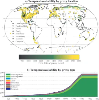
Fig. 1. Temporal and spatial availability of the M08 proxy network between 850–1800 AD. Top panel: the spatial distribution of the M08
proxies, with colored dots indicating the first year that each proxy record becomes available. Each marker represents a proxy class, as indicated in the legend. Bottom panel: the temporal availability of each proxy class.
emulation. Figure 1 shows the spatiotemporal distribution of the remaining 1138 proxies. Most proxies are concentrated in extra-tropical land regions of the Northern Hemisphere, par-ticularly across North America and western Europe (Fig. 1a). Tree-ring width is the dominant proxy class, and fewer than 200 proxies in total are available prior to 1400 AD (Fig. 1b).
2.1 Spatial characteristics
Spatial relationships between proxies (P) and temperature (T) are explored by calculating the Pearson’s correlation co-efficient (ρ) between each proxy and the HadCRUT3v sur-face temperature field (Brohan et al., 2006, the tempera-ture target used in the M08 and M09 studies). As in M08, temperature grid boxes less than 10 % complete were re-moved from the HadCRUT3v data set, and missing val-ues were infilled with the RegEM algorithm using ridge re-gression (Schneider, 2001) during the 1850–2006 AD pe-riod.ρis calculated between annually averaged HadCRUT3v
temperature observations and annual proxy data1 over the 1850–1995 AD period. The statistical significance of ρ is also taken into account, using a spectrum-preserving, non-parametric test (Ebisuzaki, 1997).
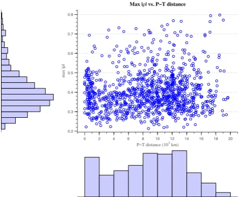
In Fig. 2,|ρ|maxis plotted as a function ofP–T distance, where|ρ|max(i)= max
j∈[1,p]
|ρ(Pi, Tj)| is the highest absolute
value of the estimated correlation coefficients between the
ith proxy and all temperature grid points. The total number of temperature grid cells isp= 1732, as in M08. All the tem-perature and proxy data can be downloaded at http://www. ncdc.noaa.gov/paleo/pubs/mann2008/mann2008.html.
Contrary to common assumptions (e.g., Jones and Mann, 2004), we find thatρ(P , T )is not a monotonically decreas-ing function of distance. As in Fig. 2, the distribution ofP–T
distance is bimodal: one cluster of proxies is well correlated to local temperature (distance shorter than 2000 km, similar to findings in Hansen and Lebedeff, 1987), but the majority of proxies are at least 8000 km away from the temperature
1M08 interpolated non-annually resolved proxies to annual
0 2 4 6 8 10 12 14 16 18 20 0.2
0.3 0.4 0.5 0.6 0.7 0.8
P−T distance (103 km)
max |
ρ
|
Max |ρ| vs. P−T distance
Fig. 2. Maximum absolute correlation coefficient|ρ|between prox-ies of the M08 network and the HadCRUT3v grid point tempera-tures vs. the corresponding distance between the proxy location and
the grid point. On theyaxis is the histogram of the maximum|ρ|;
on thexaxis is the histogram of distance between each proxyPi
and the corresponding temperature gridTj that gives the highest
|ρ|.
point yielding the highest|ρ|. On the other hand, the distri-bution of|ρ|maxis unimodal and positively skewed. The dis-tribution exhibits a mode near 0.4, while high values are quite rare (95 % ofρvalues are below 0.76). The average|ρ|max is 0.45, corresponding to aP–T distance of 11 000 km.
The counterintuitive pattern of Fig. 2 is a consequence of two effects: many proxies indeed are primarily sensitive to local temperature, but the probability of finding a spurious (non-physical) correlation also increases as the search radius increases. Some of the high non-local correlations may be reflective of long-range temperature dependencies (telecon-nections, c.f. Liu and Alexander, 2007), such as precipita-tion proxies in the southwestern United States (e.g., Cook et al., 2004, 2007, see also Fig. S23, Supplement). Others may arise by chance alone. Since we lack a theoretical crite-rion to distinguish real teleconnections from spurious corre-lations, we constructed pseudoproxies representing two end-member possibilities: one corresponding to local temperature associations, and the other mimicking each proxy’s highest potential to capture large-scale teleconnections. An alterna-tive network design, balancing the two extreme scenarios, is explored in the supplementary information (SI, Sect. 3).
Traditionally, pseudoproxies P (x, t ) are generated ac-cording to
P (x, t )=Ts(x, t )+
1
SNR ·ε(x, t ), (1)
whereTs is a time-standardized2version ofT. The primary
data ofT are grid cells extracted from GCM fields in a way that mimics instrumental data availability.ε(x, t ) are inde-pendent realizations of a Gaussian white-noise process with zero mean and unit variance, and the signal-to-noise ratio (SNR) controls the amount of noise in the pseudoproxies (Mann and Rutherford, 2002; von Storch et al., 2004; Mann et al., 2005, 2007; Rutherford et al., 2005; Küttel et al., 2007; Smerdon et al., 2008; Smerdon et al., 2011; Christiansen et al., 2009; Emile-Geay et al., 2013a). SNR is related to proxy-temperature correlationsρvia
SNR= |ρ|
p
1−ρ2. (2)
(Mann et al., 2007). While most studies have heretofore considered spatially uniform SNRs, it is clear that |ρ| is quite variable (Fig. 2), requiring pseudoproxy networks to contain such variability. In this study, spatial variations of SNRs and the bimodal pattern of Fig. 2 are explored via two end-members:
1. Local SNR: each proxy record is regressed onto tem-perature at the closest HadCRUT3v grid point over the 1850–1995 AD period, exposing each proxy’s abil-ity to record local temperature conditions (Fig. 3, top panel);
2. Max SNR: proxies are regressed onto all temperature points in the HadCRUT3v data set. The highest|ρ|for each proxy is selected to constructP (x, t )at that point (Fig. 3, bottom panel).
Temperature grid points selected in each design are then used to calculate SNR via Eq. (2). Their locations are also used to select grid cells from the simulated temperature field, which are assigned toTsin Eq. (1). In addition, the statistical
significance of ρ is also incorporated into the construction of the PPEs. Proxies showing spurious correlations are ex-cluded based on the Ebisuzaki (1997) significance test. Only the ones with a significant relationship to annual temperature in the HadCRUT3v data set are retained. Based on the sig-nificance test, only 312 out of 1138 M08 proxies exhibit a significant correlation with local temperature, whereas 1121 proxies are significantly correlated to at least one temper-ature point on Earth. Pseudoproxies are therefore sampled only at these proxy sites. Unique temperature grid points be-ing used in the local and max SNR networks reduce to 128 and 551, respectively, i.e., only locations of these tempera-ture grids are used to sampleTs in Eq. (1). As illustrated in
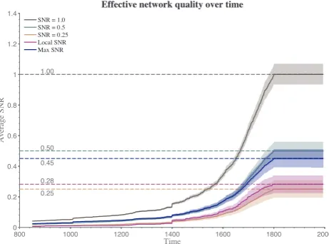
Fig. 3, even in the best-case scenario (max SNR), SNR is on average lower than 0.5, with fewer than 30 proxies exhibit-ing an SNR above 1.0. In the local SNR case, the mean SNR is even lower (0.27), close to the low end of SNRs usually considered in pseudoproxy studies (0.25).
Fig. 3. Estimated signal-to-noise ratio (SNR) for proxies in the M08 network. Top panel: Local SNR scenario, in which SNR is calculated
between each proxy and its closest temperature grid. Bottom panel: max SNR scenario, in which the highest SNR for each proxy is chosen from its correlations with all temperature grids available. Colors reflect the value of SNR assigned to each pseudoproxy, as per Eq. (2).
We emphasize that neither choice of SNR design is phys-ically realistic – instead, each may only be viewed as an end-member experiment of real-world conditions. A middle-ground scenario, balancing locality with the ability to capture the largest correlations, is explored in the SI (Sect. 3). Results based on this intermediate SNR design are found to be very similar to the max SNR case, and thus are not shown in the manuscript.
Similar characteristics were also considered in PPEs by Christiansen et al. (2009), in which empirical SNRs and noise values were used to reflect the heterogeneous proxy quality in the Mann et al. (1998) proxy network. Their work, however, did not model the temporal heterogeneity in proxy availability, and the spatial skill evaluation was not their main focus. Our study here seeks to evaluate the impact of spatial heterogeneity in multiproxy networks and its im-pact on derived CFRs. Six networks are designed to address this problem, of which two model the spatial variation of SNRs in real-world proxies (local SNR and max SNR) and four have uniform SNRs. Following previous studies (Mann and Rutherford, 2002; von Storch et al., 2004; Mann et al., 2005, 2007; Rutherford et al., 2005; Küttel et al., 2007; Smerdon et al., 2008; Smerdon et al., 2011; Werner et al., 2013), the four networks of homogenous quality are designed by assigning constant SNRs (SNR =∞, 1.0, 0.5, 0.25) in Eq. (1). These six networks together provide the basis for our experiments.
2.2 Temporal characteristics
Another realistic characteristic we incorporate into the PPE design is the temporal heterogeneity of proxy availability. As shown in Fig. 1b, data availability decreases steeply back in time, and a staircase pattern is evident for all proxy classes. In a similar manner, the effective SNR, which is the average SNR of all proxies available at a given time point, also de-clines back in time (Fig. 4). The pattern is consistent with properties of the M08 network: most of the high SNR prox-ies (such as tree rings and corals) are only available for sev-eral decades or centuries prior to widespread observational data. For instance, most tree-ring chronologies drop out of the network prior to the 16th century, with fewer than 100 (out of an original 1031) still available before the 14th ctury. Overall, only 47 proxies are available throughout the en-tire reconstruction period, of which 19 have decadal or lower resolution.
To isolate the impact of temporal availability, we specify two types of pseudoproxy networks:
1. M08 “flat” network: pseudoproxy availability is uni-form through time.
800 1000 1200 1400 1600 1800 2000 0
0.2 0.4 0.6 0.8 1 1.2 1.4
Time
Average SNR
Effective network quality over time
SNR = 1.0 SNR = 0.5 SNR = 0.25 Local SNR Max SNR
1.00
0.50 0.45
0.28 0.25
Fig. 4. Effective network quality expressed as SNR (Eq. 2) for
ide-alized pseudoproxy networks and observed networks. For the ob-served SNRs, we consider two possible scenarios as described in Sect. 2.1. Shaded areas correspond to the 2.5–97.5 percentile inter-val, providing a complete picture of effective SNR across the 100-member noise ensemble. Dashed lines correspond to the values of
SNR for temporally invariant networks. SNR =∞is not plotted.
2.3 Limitations
Despite the spatiotemporal characteristics that are modeled in the pseudoproxies, the networks are still idealized in var-ious respects. The pseudoproxy networks do not model the temporal auto-correlation (persistence) present in real-world temperature and proxy data, nor do they consider the effect of using low-resolution data for reconstructions of annual tem-perature. All pseudoproxies are generated on an annual basis without regard for the proxies’ actual resolution (as done in most other pseudoproxy studies). To more realistically model real-world proxies, future PPE designs should represent the actual resolution of each proxy (Christiansen, 2011).
Using Gaussian white noise forεin Eq. (1) is a natural first step, but a more complex noise model could be used to bet-ter reflect real-world noisy proxies (Smerdon, 2012, and ref-erences therein), as done in Tingley and Huybers (2010a, b) and Christiansen and Ljungqvist (2012). Furthermore, mech-anistic proxy models could be used to simulate synthetic proxy records with more realistic properties (Anchukaitis et al., 2006; Evans, 2007; Cobb et al., 2008; Thompson et al., 2011; Evans et al., 2013). Finally, the target field is assumed to be noise-free, yet in reality, gridded instrumental observa-tions may contain substantial noise or interpolation errors, yielding a large influence on the derived calibrations and thus the reconstruction in the preinstrumental era (Emile-Geay et al., 2013a, b). While we explore herein the impacts of significant advancements in PPE design, incorporation of the above considerations will further improve the degree to which PPEs can be interpreted as representative of real-world CFR performance.
3 Methodology
3.1 CFR techniques
Two classes of statistical methods are commonly used to perform CFRs. One is based on multivariate linear regres-sion models, where inference is performed in a frequen-tist framework (e.g., Mann et al., 1998; Mann et al., 2008, 2009; Schneider, 2001; Luterbacher et al., 2004; Smerdon et al., 2010; Guillot et al., 2013) and the other uses Bayesian hierarchical models (BHMs, e.g., Li et al., 2010; Tingley and Huybers, 2010a). We restrict our attention to frequentist regression-based methods since only those have heretofore been used to derive global/hemispheric CFRs.
LetP be annp×ppmatrix of proxy values andT be an
nt×ptmatrix of instrumental temperature records, wherenp
andnt are the number of years of available data (i.e.,
num-ber of observations),ppandpt are the number of spatial
lo-cations (i.e., number of variables), and the subscriptspand
t denote proxies and instrumental data, respectively. Tradi-tional regression-based CFR methods assume a multivariate linear relationship between proxies and the climate variable of interest: e.g., temperature (Jones and Mann, 2004; Na-tional Research Council, 2006; Jones et al., 2009; Tingley et al., 2012). Additionally, each year is often treated as an in-dependent observation. In this context, temperature may be estimated from the proxies via the regression equation:
T =B P +ε, (3)
whereεis an error term following a multivariate normal dis-tribution with zero mean. In the sample-rich setting famil-iar to classic regression problems (e.g., Anderson, 2003), the optimal estimate ofB would be given by the ordinary least squares (OLS) estimate:
b
B =
P>cPc
−1
P>cT , (4)
where Pc is the submatrix of P spanning the calibration
interval. This formulation is such that in order to estimate
b
B, P>cPc must be invertible (non-singular). In paleoclimate
applications, however, it is often the case that P>cPc is
rank-deficient, (i.e., not invertible): instrumental temperature records are only available for the past 150 yr or so (nt≈150),
and the number of proxiesppis on the order of 103(high
3.1.1 RegEM
RegEM (Schneider, 2001) is a variant of the EM algorithm (Dempster et al., 1977; Little and Rubin, 2002) designed for the imputation of missing values in spatiotemporal data sets typically encountered in climatology. Under the multivariate normal assumption, given an initial estimate of the meanµˆ and the covariance matrixb6, the RegEM algorithm reduces
to regressing the missing values onto the available ones (in-strumental temperature data and overlapping proxies)3. The estimates ofµˆ andb6are updated at each iteration until
con-vergence is achieved. Two regularization methods have been considered in RegEM: one is ridge regression (Tikhonov and Arsenin, 1977; Hoerl and Kennard, 1970a, b), used in the paleoclimate context by Mann and Jones (2003), Rutherford et al. (2003), Mann et al. (2005) and Rutherford et al. (2005); the other is truncated total least squares (Van Huffel and Vandewalle, 1991; Fierro et al., 1997, hereinafter TTLS), used in the paleoclimate context by Mann et al. (2007, 2008, 2009), Wilson et al. (2010) and Emile-Geay et al. (2013a, b). Rutherford et al. (2010), Christiansen et al. (2010) and Tingley et al. (2012) have also discussed the relative mer-its of these methods. As explained in Smerdon and Kaplan (2007), Mann et al. (2007) and Smerdon et al. (2008), ridge regression can lead to overly damped reconstructions in very data-sparse scenarios such as paleoclimate reconstructions. TTLS mitigates such variance losses, and therefore is chosen as our regularization method for this study. We employ two different styles of RegEM-TTLS: one following the standard formulation described in Schneider (2001), and the other fol-lowing its paleoclimate-specific implementation described in Mann et al. (2009).
3.1.2 M09 implementation of RegEM-TTLS
The M09 implementation of TTLS uses a hybrid version of RegEM-TTLS (Mann et al., 2007) that treats low-frequency and high-frequency signals separately (the domains are split at a 20 yr period). The reconstruction is then performed in a forward stepwise approach century by century. For each step, the target data are compressed in that only the firstMleading modes of surface temperature are retained, whereMis an es-timate of the number of degrees of freedom in the proxy net-work, determined by a fit to its log-eigenvalue spectrum. Ad-ditionally, semi-adaptive choices are adopted for both low-frequencykl and high-frequency truncation parameters kh.
The method selects (1)klto retain 33 % of the low-frequency
multivariate data variance (Mann et al., 2009; Rutherford et al., 2010); and (2) khby detecting the first break in the
log-eigenvalue spectrum of high-frequency multivariate data variance.
3µ∈ <1×pis the temporal mean of thep=p
p+pt variables
to be estimated, while6 ∈ <p×pis the corresponding covariance
matrix.
Although these ad hoc modifications are not grounded in statistical theory, the M09 implementation of TTLS has proven effective in practice (Mann et al., 2009; Emile-Geay et al., 2013a, b). Indeed, the M09 implementation is the only technique that has ever been used for global-scale, real-world CFRs, so it is taken as the benchmark of our study. By com-paring M09 to TTLS with fixed regularization (i.e., RegEM-TTLS), we investigate the merits of the M09 approach to pa-rameter selection in an ensemble framework, which is a novel assessment of this heuristic approach.
3.1.3 CCA
CCA (Christiansen et al., 2009; Smerdon et al., 2010) is based on ideas presented in Barnett and Preisendorfer (1987). As discussed in Smerdon et al. (2010), CCA employs singu-lar value decomposition (SVD) to perform dimensional re-ductions separately onT,P, andB. The basic assumption, as in most paleoclimate applications, is that the first few lead-ing modes of EOF-PC pairs contain most of the variance in the target climate field and the multiproxy network. The al-gorithm seeks an optimal set of truncation parameters (dt,dp,
dcca) that yields good approximations ofT,P, andB,
respec-tively. These truncation parameters are chosen by minimiz-ing the area-weighted root mean square error (RMSE) of the reconstruction relative to the target field using a leave-half-out cross-validation procedure (e.g., Chap. 7, Hastie et al., 2008).
Smerdon et al. (2010); Smerdon et al. (2011) have only ap-plied CCA on pseudoproxy networks with constant temporal availability. For this study, we modify the original CCA code to make it applicable to real networks with variable temporal availability, and also made it more computationally efficient. Readers are referred to the SI for more details.
3.1.4 GraphEM
GraphEM (Guillot et al., 2013) is based on the theory of Gaussian graphical models (GGMs, a.k.a. Markov random fields, Whittaker, 1990; Lauritzen, 1996). A GGM makes use of the conditional independence4 structure of the cli-mate field, in order to reduce the dimensionality and obtain a parsimonious estimate of≡6−1. The conditional inde-pendence relations are estimated by solving an`1-penalized
maximum likelihood problem (Friedman et al., 2008).6 is then estimated in accordance with these conditional inde-pendence relations. The resulting 6b is sparse and
better-conditioned, and therefore is applicable within the OLS framework. This procedure is implemented within the stan-dard EM algorithm without further need for regularization. GraphEM was extensively tested against RegEM-TTLS in
4Conditional independence: two random variablesXandY are
“conditionally independent” given a random variableZif, onceZ
is known, the value ofY does not add additional information about
Guillot et al. (2013), albeit with the more idealized proxy design of Smerdon et al. (2011). One goal of this study is to document GraphEM’s performance in a more realistic context.
3.2 Numerical experiments
As in Smerdon et al. (2011), all of our pseudoproxy ex-periments target the annual surface temperature field com-puted from the NCAR CSM1.4 integration of Ammann et al. (2007), using the correctly oriented version of the CSM1.4 field (Smerdon et al., 2010). Although multiple last millennium simulations are becoming publicly available as part of the Paleoclimate Modelling Intercomparison Project Phase 3 (PMIP3) and through other projects (Fernández-Donado et al., 2013), we selected the CSM1.4 model to en-able comparisons with previous work (Mann et al., 2005, 2007; Lee et al., 2008; Mann et al., 2009; Li et al., 2010; Ammann et al., 2010; Smerdon et al., 2010; Smerdon et al., 2011). The target field was spatially masked to approximate the availability of the HadCRUT3v data set used in the Mann et al. (2009) study. We generated 100 realizations of pseudo-proxy series for each SNR case (SNR =∞, 1.0, 0.5, 0.25, lo-cal SNR and max SNR) by varyingεin Eq. (1), and then per-formed reconstructions with the four CFR techniques. The first four cases have fixed SNR, corresponding to networks of homogeneous quality.
The ensemble approach allows us to identify spurious re-construction skill arising from random noise, and to test the robustness of each method. We also conducted experiments using both the flat and staircase networks. Experiments using the flat network, in which the spatial distribution of pseudo-proxies is temporally invariant, serve as the control group in this study. Experiments with the staircase network, corre-spondingly serve as the test group. By comparing results be-tween these two experiments, we test the null hypothesis that temporal heterogeneity does not affect reconstruction skill.
Reconstruction and calibration intervals are 850–1849 AD and 1850–1995 AD, respectively. Annual means of temper-ature and pseudoproxies are used for the reconstructions. The same input data are assigned to each CFR method, and standardization (if necessary) is performed internally in each method. Reconstructions are referenced to zero over the cal-ibration interval. Possible trends during the calcal-ibration inter-val are not removed. We also consider computational cost, and investigate numerical methods to speed up each CFR technique. Further details are provided in the SI.
4 Results
4.1 Skill metrics
As is common practice in paleoclimatology, we evaluate construction skill using the coefficient of efficiency (CE), re-duction of error (RE) and the coefficient of determination
Table 1. Comparison betweenR2, RE, and CE.yi denotes theith
temperature grid point, andyˆidenotes the estimation ofyi.ycand
yv refer to the mean of (y1, y2, . . . ,yn) over the calibration
pe-riod and verification pepe-riod, respectively. Adapted from National Research Council (2006), Chap. 6.
Metric Expression Range Tracks
R2
" n P
i=1
(yi−yv)
ˆ
yi− ˆyv
#2
n P
i=1
(yi−yv)2
n P
i=1
ˆ
yi− ˆyv
2 [0,1] Phase
RE 1−
n P
i=1
(yi− ˆyi)2
n P
i=1
(yi−yc)2
[−∞, 1] Phase and amplitude
CE 1−
n P
i=1
(yi− ˆyi)2
n P
i=1(
yi−yv)2
[−∞, 1] Phase, amplitude and mean
(R2) (Cook et al., 1994; Bürger, 2007). These validation statistics (Table 1) are related to the mean squared error (MSE) that is commonly used for statistical analysis. They are calculated for both the global mean temperature index and the spatial field; the former provides an aggregate sum-mary of a method’s ability to track global climate fluctua-tions, and the latter evaluates a method’s spatial performance. The global mean enables comparisons with index tions, which comprise the majority of published reconstruc-tions of hemispheric and global temperatures (Fig. 6.10 in Jansen et al., 2007).
As indicated in Fig. 3, the quality of pseudoproxies in the local SNR case, on average, is comparable with the SNR = 0.25 network, and the average SNR of pseudoprox-ies in the max SNR case is similar to the SNR = 0.5 net-work. Based on these considerations, we only show results from the spatially heterogenous pseudoproxy networks. The reader is referred to the SI for results on spatially homoge-nous networks.
4.2 Reconstructing the global mean
Temp. Anom. (K)
Global mean temperature (20-year lowpass), staircase network
-0.4 -0.2 0 0.2 0.4
900 1000 1100 1200 1300 1400 1500 1600 1700 1800 1900 2000
Time (year A.D.)
-0.4 -0.2 0 0.2 0.4
Temp. Anom. (K)
b) max SNR
a) Local SNR RegEM-TTLSM09
CCA GraphEM Target
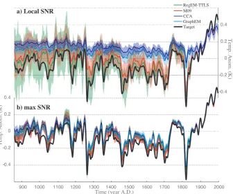
Fig. 5. Area-weighted global mean time series comparison of the four CFR methods, with the staircase network. (a) local SNR, (b) max
SNR. Only the low-frequency (20 yr lowpass) signal is plotted. Black line: target temperature from the CSM1.4 model output; colored lines: reconstructed temperature from median of the reconstruction ensembles; shaded areas: 2.5–97.5 percentiles derived from the reconstruction ensembles.
and thus a correspondingly smaller MSE. Overall, M09 pro-duces the most skillful global mean temperature series in both cases, closely followed by RegEM-TTLS. It would be erroneous, however, to conclude that these two methods pro-duce the closest match to the target, as there is a large spread between different noise realizations.
In assessing the risk properties of each method (Fig. 5a), we find that GraphEM and CCA are more consistent estima-tors than RegEM-TTLS and M09: their ensemble spreads are much narrower, especially for early reconstruction intervals (prior to 1600 AD). This indicates that any given RegEM-TTLS or M09 reconstruction may yield an inaccurate depic-tion of the true temperature, and this risk should be kept in mind especially when using M09 and RegEM-TTLS for real-world reconstructions.
4.3 Spatial performance
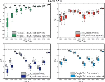
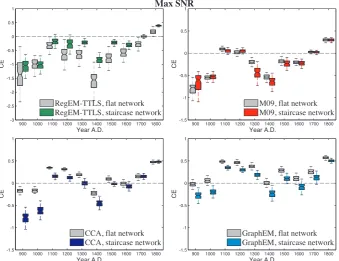
We now examine the spatial performance of the four CFRs. In Figs. 7 and 8, we summarize the century-by-century skill variation and each CFR’s ensemble spread using box plots of the globally averaged CE statistic. CE is shown because it is the most stringent metric among the three in Table 1 (Cook et al., 1994; Ammann and Wahl, 2007), and thus exposes
significant contrast between methods (Table S1, Supple-ment). Box plots characterize the full distribution of the 100-member ensemble: the median of each distribution assesses the tendency for temporal proxy availability to affect recon-struction skill, while the spread yields information about the consistency of each method. The impact of spatial hetero-geneities is isolated by plotting spatial maps of CE using the flat network in Figs. 9 and 10, which help us trace spatial errors and inter-method similarities and differences.
4.3.1 Effect of temporal heterogeneities
Verification statistics for the global mean time series (20-year lowpass)
Local Max
-4 -3 -2 -1 0 1
CE RegEM-TTLS
M09 CCA GraphEM
Local 0.4
0.6 0.8 1
RE RegEM-TTLS
M09 CCA GraphEM
Local 0.4
0.6 0.8 1
R
2
RegEM-TTLS M09 CCA GraphEM
Local 0
0.02 0.04 0.06
Bias
2
RegEM-TTLS M09 CCA GraphEM
Local 0
0.005 0.01 0.015 0.02
Variance
RegEM-TTLS M09 CCA GraphEM
Local 0
0.02 0.04 0.06 0.08
MSE
RegEM-TTLS M09 CCA GraphEM
Max Max
Max
Max Max
Fig. 6. Summary of verification statistics of the global mean temperature reconstruction ensemble. Note the range of ordinates for each metric
is different. MSE = variance+bias2.
900 1000 1100 1200 1300 1400 1500 1600 1700 1800 -18
-16 -14 -12 -10 -8 -6 -4 -2 0
CE
Year A.D.
RegEM-TTLS, flat network RegEM-TTLS, staircase network
900 1000 1100 1200 1300 1400 1500 1600 1700 1800 -5
-4 -3 -2 -1 0 1
CE
Year A.D.
M09, flat network M09, staircase network
900 1000 1100 1200 1300 1400 1500 1600 1700 1800 -5
-4 -3 -2 -1 0 1
CE
Year A.D.
CCA, flat network CCA, staircase network
900 1000 1100 1200 1300 1400 1500 1600 1700 1800 -5
-4 -3 -2 -1 0 1
CE
Year A.D.
GraphEM, flat network GraphEM, staircase network Local SNR
Fig. 7. Temporal variation of globally averaged CE, within CFRs derived from the local SNR network. Spatial CE is first calculated for each
grid box, and then global averages are calculated using area-weighted means. Each box plot represents CE scores from the 100-member ensemble for each 100 yr slice between 850 and 1850 AD. For example, the box plot with time slice 900 corresponds to the global mean CE
900 1000 1100 1200 1300 1400 1500 1600 1700 1800 -3
-2.5 -2 -1.5 -1 -0.5 0 0.5 1
CE
Year A.D.
RegEM-TTLS, flat network RegEM-TTLS, staircase network
900 1000 1100 1200 1300 1400 1500 1600 1700 1800 -1.5
-1 -0.5 0 0.5 1
CE
Year A.D.
M09, flat network M09, staircase network
900 1000 1100 1200 1300 1400 1500 1600 1700 1800 -1.5
-1 -0.5 0 0.5 1
CE
Year A.D.
CCA, flat network CCA, staircase network
900 1000 1100 1200 1300 1400 1500 1600 1700 1800 -1.5
-1 -0.5 0 0.5 1
CE
Year A.D.
GraphEM, flat network GraphEM, staircase network Max SNR
Fig. 8. Same as Fig. 7, but for the max SNR network.
forcing events, which may have more coherent spatial ex-pressions than other fluctuations, appear to be more easily captured by the proxy network. This suggests that recon-struction skill is not only affected by proxy availability and quality, but is also a function of the type and amplitude of climate variations (i.e., internally generated vs. externally forced variations). See Sect. 4 in the SI for more discussions. An additional important observation to note is that RegEM-TTLS in the local SNR case is distinct from the other three methods (Fig. 7) in that the temporal availabil-ity of input data dominates the reconstruction skill, which is a monotonically increasing function of time. The ensem-ble spread becomes wider back in time as well (consistent with Fig. 5a). The decreasing trend back in time for RegEM-TTLS is partially due to the fact that the method uses a fixed truncation parameter for the estimation ofb6, despite
the declining availability (Fig. 3) and quality (Fig. 4) of pseudoproxies back in time. Consequently, the TTLS solu-tion tends to be less regularized, and hence is dominated by noise (Sima and Van Huffel, 2007). For GraphEM, a fixed graph is used for the entire reconstruction interval. The graph identifies most of the significant proxy-temperature relation-ships and thus GraphEM is able to efficiently use the re-lationships for reconstruction. M09 and CCA, on the other hand, have semi-adaptive and adaptive criteria respectively when performing reconstructions, and are less sensitive to temporal heterogeneities in the pseudoproxies. In the max SNR case (Fig. 8), RegEM-TTLS shows a similar pattern to the other CFRs. This implies that for RegEM-TTLS, the
reconstruction skill vs. data availability relationship is con-ditionally dependent on data quality: when proxy quality is relatively high (max SNR), reconstruction skill is relatively insensitive to the choice of truncation parameters in RegEM-TTLS, but – like other CFRs – the skill is still sensitive to high-amplitude climate events.
Despite similarities across reconstructions of global mean temperature (Figs. 5b, 6; max SNR columns), the spatial metrics reveal large discrepancies among methods. Although M09 and RegEM-TTLS perform well reconstructing the global mean temperature, their globally averaged spatial skill only breaches zero in the last two centuries of the reconstruc-tion, even in the max SNR case (Fig. 8). GraphEM and CCA, on the other hand, display high spatial skill for most of the reconstruction period (in the max SNR case, Fig. 8).
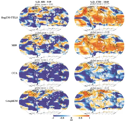
4.3.2 Effect of spatial heterogeneities
To isolate the effect of spatial heterogeneities, and to bet-ter visualize spatial patbet-terns, Figs. 9 and 10 display the spa-tial pattern of CE using the flat network over the first (850– 949 AD) and last centuries (1750–1849 AD) of the recon-struction5. In Fig. 9, a band of high CE scores connecting the eastern equatorial Pacific to North America is evident in all cases, and appears to be a feature of CSM1.4’s climate (Smerdon et al., 2011). Similarly, there is some reconstruc-tion skill over other oceans where no proxies are available.
5Spatiotemporal maps for each century of the entire
Fig. 9. Spatial pattern of CE, based on ensemble median using the local SNR flat network. 850–949 and 1750–1849 AD represent periods
with the minimum and maximum global mean CE over the entire reconstruction interval, respectively.
Collectively, this indicates that modeled teleconnections are effectively exploited by all methods to reconstruct surface temperature in regions with little to no proxy coverage. How-ever, the pattern of enhanced skill associated with ENSO (El Niño–Southern Oscillation) teleconnections vanishes in the 850–949 AD interval when employing RegEM-TTLS or M09 on the max SNR network (Fig. 10), but is still visible in CFRs using CCA and GraphEM. This suggests that the latter two methods are more skillful in resolving such spatial patterns.
Using the local SNR network, we find that RegEM-TTLS and M09 both produce more skillful reconstructions than GraphEM and CCA. In the case of max SNR, how-ever, the results are opposite: reconstructions with CCA and GraphEM are more skillful. In particular, GraphEM is the most skillful method almost everywhere (Fig. 10) and across all time intervals (Figs. 8, S10, Supplement). The goal of
dimension reduction in CCA is to increase the solution stabil-ity, and is achieved by pre-filtering noise and retaining only a few leading modes. Similarly, GraphEM filters out spuri-ous proxy-temperature relationships and noise by assigning zeros in the precision matrix (Friedman et al., 2008; Hastie et al., 2008; Guillot et al., 2013). In the case of the local SNR network, most proxies have SNRs lower than 0.3 (or equiva-lently, more than 92 % noise6), and hence are dominated by random noise. As a consequence, both CCA and GraphEM tend to treat those proxies as noise and filter them out, shrink-ing the reconstruction closer to the calibration mean. Fig-ures 9 and 10 suggest that RegEM-TTLS and M09 are likely to be more powerful when data are very noisy (the local SNR network). Nevertheless, the poor risk properties of these two
6%noise: the fraction of the variance in the proxy accounted for
by the noise component alone, formulated as 1
1+SNR2 (Mann et al.,
Fig. 10. Same as Fig. 9, but for the max SNR flat network.
methods, as discussed above, indicate that single inferences drawn with these methods should be treated with caution.
Despite the differences among methods described above, some common features emerge when comparing reconstruc-tions with the realistic SNRs to uniform SNR networks (Figs. S9–S12, Supplement)7. Compared with CFRs using the SNR = 0.25 network (Fig. S11, Supplement), CFRs using the local SNR network (Fig. S9, Supplement) produce simi-lar results but are less skillful. This is primarily due to the fact that the local SNR network contains only 312 records, while the SNR = 0.25 network includes all 1138 proxies in the M08 database. The comparison between CFRs with SNR = 0.5 (Fig. S12, Supplement) and max SNR networks (Fig. S10, Supplement), however, shows that reconstructions using the max SNR network are much more skillful, especially during early reconstruction periods. We discuss this point below.
7Reconstructed patterns are relatively consistent between
meth-ods, thus we only present results from GraphEM in this paper.
5 Discussion
Sampling the same grid cells multiple times effectively in-creases the SNR for those grid cells, and thus may contribute to the reconstruction skill. This feature is expected to oper-ate in nature as well, however, and provides additional mo-tivation for replicating proxy records. Additionally, we note again that such conclusions might be model-dependent. The skill observed here may result from the low internal variabil-ity in the NCAR CSM1.4 model (partially a consequence of its low resolution). To confirm these findings, similar experi-ments will be conducted with PMIP3-generation last millen-nium simulations (http://pmip3.lsce.ipsl.fr/).
We also find that differences across CFRs are much smaller in the case of the max SNR network (Fig. 10), in-dicating that, not surprisingly, reconstructions are much less sensitive to methodology when data quality is high. The spa-tial reconstruction skill, as expected, is highest in regions of dense proxy availability (e.g., North America), which is consistent with previous findings by Smerdon et al. (2011). The contrast between Figs. 9 and 10, both assuming constant time availability, suggests that our CFR methods, in partic-ular GraphEM and CCA, are more sensitive to data quality than to temporal availability.
As mentioned in Sect. 4.3.1, the ensemble spread for each method is quite different. RegEM-TTLS consistently yields the largest spread, followed by M09, CCA and GraphEM. As an error-in-variable model (EVM), TTLS is designed to minimize the variance of residuals from both the predictands (Tˆ −T) and the predictors (Pˆ −P). The minimization is subject to the estimates of regression coefficients, which in turn depend crucially on the choice of the truncation param-eter. Since the noise εin Eq. (3) is randomly generated, it is sometimes spuriously high in the calibration interval and makes the true signal too noisy for CFR methods to iden-tify, especially in the local SNR network. Under such cir-cumstances, reconstructions using TTLS with fixed trunca-tion may therefore be over-fitting to noise. This confirms an important point made by Christiansen et al. (2009): there is a substantial element of stochasticity in the reconstructions. Hence, one might obtain very different results with the same method applied to different pseudoproxy noise realizations or to different jackknifed proxy networks in real-world re-constructions. In order to improve reconstruction skill when employing RegEM-TTLS, we suggest the development of an algorithm that adaptively selects the regularization parame-ters using standard statistical theory.
Compared with RegEM-TTLS, M09 produces more skill-ful reconstructions. In particular, M09 appears advantageous at very high noise levels (local SNR; Figs. 7, S6, Supple-ment). This is not surprising in part due to the heuristic truncation choices. M09 strongly benefits from the hybrid-frequency approach to perform reconstructions, namely white noise contained in the low-frequency pseudoproxies is effectively filtered out and hence the low-frequency compo-nents are better reconstructed in the PPEs. The noise-filtering advantage is likely not present in real-world reconstructions,
and the absence of a theoretical justification for the selection criterion makes it vulnerable. Given a different data set or given a different noise model (by varyingε in Eq. (1), for instance, using red noise instead), the 20 yr frequency split might no longer be optimal, and the “33 %-truncation” crite-rion might also need to change. For the global mean tempera-ture, M09 produces the closest fit to the target overall (Fig. 5), which is due to the fact that truncation parameters are opti-mized to fit the global mean. However, our results suggest that the optimization comes at the expense of spatial skill, es-pecially during the early reconstruction period (Figs. 10, S5, Supplement).
Reconstructions derived from CCA and GraphEM in gen-eral show very similar results, with GraphEM slightly out-performing CCA. In particular, as shown in Figs. 8 and 10, in the max SNR case, GraphEM outperforms other meth-ods at all locations across all time intervals. This indicates that given enough high-quality data, GraphEM can produce the most skillful reconstructions. The strength of GraphEM is especially noticeable in regions of dense proxy sampling. For instance, over North America (Fig. S10, Supplement), the other three methods display negative CE scores prior to 1650 AD, yet GraphEM displays positive CE scores over the entire reconstruction interval. Nevertheless, as noted in Fig. 9, GraphEM does not perform as well in the local SNR setting as it does using the max SNR network. GraphEM’s superior performances in the former case and unsatisfying performances in the latter are both largely due to the graphi-cal structure selected by the GraphEM algorithm. In the max SNR case, pseudoproxies have, by design, much higher SNR than they do in the local SNR case. Thus most of the sig-nificant proxy-temperature relationships are effectively de-tected and exploited by the method. In the local SNR case, on the other hand, very few significant relationships are de-tected and thus GraphEM fails to produce meaningful CFRs. Despite sensitivity to data quality, another potential cause of GraphEM’s poor performance in the local SNR cases is the choice of the graph. Currently, as described in Guillot et al. (2013), the graph is a fixed choice for the entire reconstruc-tion period, which is based solely on instrumental proxy-temperature relationships. To improve the performance of GraphEM-based CFRs, adaptive choices of the graph should be made for each century of the reconstruction. Through this approach, available proxies from each century will be more effectively used. Alternative methods should also be explored to estimate the graph.
Table 2. Verification statistics summary for the global mean
tem-perature time series, using the staircase network. CE, RE,R2and
bias are computed for the frequency component (20 yr low-pass) of the reconstructed global mean. All numbers given outside of parentheses are the mean of the 100-member ensemble; numbers in parentheses are the corresponding standard deviation.
Method SNR CE RE R2 bias
RegEM-TTLS
∞ +0.920.00 +0.990.00 +0.920.00 +0.020.00 1.0 +0.840.02 +0.980.00 +0.910.01 +0.030.01 0.5 +0.780.07 +0.970.01 +0.870.03 +0.030.02 0.25 +0.530.13 +0.940.02 +0.700.06 +0.040.02 local −0.120.39 +0.850.05 +0.520.09 +0.060.03 max +0.550.13 +0.940.02 +0.870.04 +0.070.01
M09
∞ +0.930.00 +0.960.00 +0.880.00 +0.020.00 1.0 +0.740.02 +0.970.00 +0.880.01 +0.050.02 0.5 +0.690.07 +0.960.01 +0.850.02 +0.050.01 0.25 +0.300.21 +0.910.03 +0.670.08 +0.070.02 local −0.240.26 +0.830.04 +0.570.06 +0.110.02 max +0.740.06 +0.970.01 +0.900.03 +0.050.01
CCA
∞ +0.960.00 +1.000.00 +0.970.00 +0.010.00 1.0 +0.780.04 +0.970.01 +0.940.01 +0.050.01 0.5 −0.180.12 +0.840.02 +0.880.02 +0.130.01 0.25 −2.920.28 +0.470.04 +0.610.06 +0.240.01 local −3.280.25 +0.420.03 +0.540.06 +0.250.01 max +0.370.07 +0.920.01 +0.910.01 +0.090.01
GraphEM
∞ +0.950.00 +0.990.00 +0.970.00 +0.010.00 1.0 +0.680.07 +0.960.01 +0.950.01 +0.060.01 0.5 +0.530.10 +0.940.01 +0.900.01 +0.080.01 0.25 −0.430.38 +0.810.05 +0.750.04 +0.140.02 local −2.000.30 +0.600.04 +0.640.05 +0.210.01 max +0.530.09 +0.940.01 +0.940.01 +0.080.01
expected: the method regularizes by maximizing the cross-correlation between the proxy and target matrices, but with-out further constraining the variance. One possible modifica-tion would be matching the variance of CCA reconstrucmodifica-tions to the variance of the target data in each grid cell during the calibration interval. In doing this, more variance would be preserved for networks affected by declining data availabil-ity. However, this modification would inflate errors and the solution could no longer be interpreted as minimizing the calibration misfit.
By contrasting the CFRs derived from four methods in both the spatial and temporal context, we find that, despite some general agreements (Fig. 5b) and reasonable skill (Ta-ble 1) in the global mean temperature reconstruction, the four methods yield large spatial differences, and their validation scores in terms of CE can still be large locally. This confirms previous findings in Smerdon et al. (2011), that the global mean temperature series is a poor indicator of spatial skill, and that spatial performance metrics are crucial for the as-sessment of different CFR techniques (e.g., Li and Smerdon, 2012). The results also highlight the difficulty in jointly op-timizing the spatial skill and the global mean temperature. Fundamentally, reconstruction skill can be assessed using MSE. As discussed in the previous paragraph, in order to find the lowest MSE (thus the best reconstruction), a tradeoff
must be found between bias and variance. It therefore is most likely that the lowest MSE for the spatial field and the global mean time series are not given by the same set of regulariza-tion parameters.
We also calculated a suite of diagnostics for reconstruc-tion skill and its dependence on (1) the number of proxies, (2) the average SNR, and (3) the sum of SNR in each grid box. No apparent relationships between these variables and spatial skill were found (Figs. S15–S20, Supplement). Our experiments also highlight the need for methodological re-finements, since no method can consistently perform well in all cases for both index and field reconstructions. We find that both RegEM-TTLS and M09 produce meaningful global mean reconstructions, but do not perform as well in the spa-tial field. The disagreement between the field and index re-construction was explored in Guillot et al. (2013), in which it is found that the skillful performance of TTLS-based global mean temperature reconstructions involves considerable can-cellation between positive and negative deviations from the true field at any given grid point (see Supplement). Hence, the fidelity of the reconstructed global mean is a poor indica-tion of spatial skill (Figs. S21, S22, Supplement).
6 Conclusions
An updated pseudoproxy network design has been con-structed with more realistic characteristics: for the first time, pseudoproxies were sampled with spatiotemporal characteristics that reflect heterogeneities in proxy quality and proxy attrition back in time. The updated network has allowed an assessment of the spatial performance of four different CFR techniques using a comprehensive suite of experiments.
Results based on the max SNR network show rela-tively small CFR sensitivity to the choice of methodology when SNR is high. However, results are strongly method-dependent in sample-starved settings. Overall, reconstruc-tions are generally better in regions with dense proxy sam-pling, although teleconnections are also exploited by these CFR methods, in particular CCA and GraphEM, to derive spatial skill outside of directly sampled regions.
The effect of temporal heterogeneities of proxy availabil-ity is counterintuitive. We find that despite the declining data availability back in time, reconstruction skill does not necessarily follow suit. Rather, our experiments show that forced, high-amplitude climatic events have a larger impact on reconstruction skill and are more easily resolved by these methods, even when data availability is low. This conclusion is nevertheless model-dependent, and needs to be verified with PPEs using output from other GCMs.
Our experiments also show that no method universally out-performs another, and that each method has its own strengths and weaknesses. Overall, RegEM-TTLS and M09 produce more skillful index reconstructions (global mean tempera-ture, Fig. 6), and retain a higher skill than other methods when proxies are very noisy (local SNR network, Fig. 9). However, RegEM-TTLS displays large ensemble spreads, partially due to its fixed choice of truncation parameter and high sensitivity to noise in the data. This emphasizes the high risk associated with conclusions from a single noise realiza-tion (such as a real-world reconstrucrealiza-tion). The stochasticity of a reconstruction method should therefore always be se-riously considered when evaluating a real-world reconstruc-tion (Christiansen et al., 2009).
The heuristic parameter choices proposed by M09 show the potential for RegEM-TTLS to produce meaningful global mean temperature reconstructions. The setup never-theless deviates greatly from the standard implementation of RegEM-TTLS. Additionally, for global mean reconstruc-tions, both RegEM-TTLS and M09 involve error cancella-tions that are not readily noticeable (Sect. 2.4 in the Sup-plement, Figs. S21, S22). This might explain some of the observed divergence between the quality of index and field reconstructions using these methods.
CCA and GraphEM generally produce very similar re-sults, but the former suffers from larger variance losses and associated mean biases. This can be attributed to the man-ner in which the method selects for the optimal estimates of
regression coefficientsBb. Given enough high-quality data,
reconstructions using GraphEM display a higher spatial skill than the other three methods everywhere in the field, and in particular over the oceans and regions with denser proxy sampling. This suggests that the reconstruction strongly ben-efits from the improved covariance estimation induced by the use of Gaussian graphical models.
Given the large performance differences among various CFR methods in the pseudoproxy context, we emphasize that unless reconstructions with various methods provide very similar spatiotemporal information, real-world reconstruc-tions derived from a single method should be viewed with caution. In agreement with Smerdon et al. (2011), we rec-ommend applying as many methods as possible to make ro-bust conclusions. Additionally, the exact pattern of spatial skill varies according to the GCM simulation used as the ba-sis of the PPEs. Multiple PMIP3 last millennium simulations should ideally be used to validate the present results. Future studies should also rigorously model real-world conditions, including persistence, noise characteristics, and a mechanis-tic representation of climate proxies. Finally, we emphasize the fundamental difficulty in finding a bias-variance trade-off that optimizes the reconstruction of both the temperature field and its global mean. Future studies should explore solu-tions that jointly minimize spatial and temporal errors.
Supplementary material related to this article is available online at http://www.clim-past.net/10/1/2014/ cp-10-1-2014-supplement.pdf.
Acknowledgements. The authors thank Sylvia Dee and
Adam Vaccaro for comments that improved the presentation of this manuscript, and also thank Sandrah Eckel and Gareth James for their statistical insight. The authors acknowledge NSF awards AGS1003818 and AGS0902436, NOAA grant NA10OAR4320137, and computational resources from the USC High Performance Computing Center.
Edited by: S. Bronnimann
References
Ammann, C. M. and Wahl, E.: The importance of the geophysical context in statistical evaluations of climate reconstruction pro-cedures, Climatic Change, 85, 71–88, doi:10.1007/s10584-007-9276-x, 2007.
Ammann, C. M., Joos, F., Schimel, D. S., Otto-Bliesner, B. L., and Tomas, R. A.: Solar influence on climate during the past millennium: Results from transient simulations with the NCAR Climate System Model, Proc. Nat. Acad. Sc., 104, 3713–3718, doi:10.1073/pnas.0605064103, 2007.
Anchukaitis, K. J., Evans, M. N., Kaplan, A., Vaganov, E. A., Hughes, M. K., Grissino-Mayer, H. D., and Cane, M. A.: Forward modeling of regional scale tree-ring pat-terns in the southeastern United States and the recent influ-ence of summer drought, Geophys. Res. Lett., 33, L04705, doi:10.1029/2005GL025050, 2006.
Anderson, T.: An Introduction to Multivariate Statistical Analysis, 3rd Edn., John Wiley & Sons, Inc., New York, 2003.
Annan, J. D. and Hargreaves, J. C.: Identification of climatic state with limited proxy data, Clim. Past, 8, 1141–1151, doi:10.5194/cp-8-1141-2012, 2012.
Barnett, T. P. and Preisendorfer, R.: Origins and Levels of Monthly and Seasonal Forecast Skill for United States Surface Air Tem-peratures Determined by Canonical Correlation Analysis, Mon. Weather Rev., 115, 1825–1850, 1987.
Bradley, R. S.: Are there optimum sites for global paleotemperature reconstruction?, vol. 41 of NATO ASI, chap. Climate variations and forcing mechanisms of the last 2000 years, Springer, Berlin, Heidelberg, New York, 603–624, 1996.
Briffa, K. R., Osborn, T. J., Schweingruber, F. H., Harris, I. C., Jones, P. D., Shiyatov, S. G., and Vaganov, E. A.: Low-frequency temperature variations from a northern tree ring density network, J. Geophys. Res., 106, 2929–2942, doi:10.1029/2000JD900617, 2001.
Brohan, P., Kennedy, J. J., Harris, I., Tett, S. F. B., and Jones, P. D.: Uncertainty estimates in regional and global observed tempera-ture changes: A new data set from 1850, J. Geophys. Res., 111, D12106, doi:10.1029/2005JD006548, 2006.
Bürger, G.: On the verification of climate reconstructions, Clim. Past, 3, 397–409, doi:10.5194/cp-3-397-2007, 2007.
Christiansen, B.: Reconstructing the NH Mean Temperature: Can Underestimation of Trends and Variability Be Avoided?, J. Cli-mate, 24, 674–692, doi:10.1175/2010JCLI3646.1, 2011. Christiansen, B.: Reply to “Comments on ‘Reconstructing the
NH Mean Temperature: Can Underestimation of Trends and Variability be Avoided?”’, J. Climate, 25, 3447–3452, doi:10.1175/JCLI-D-11-00162.1, 2012.
Christiansen, B. and Ljungqvist, F. C.: Reply to “Comments on ‘Re-construction of the Extratropical NH Mean Temperature over the Last Millennium with a Method That Preserves Low-Frequency Variability”’, J. Climate, 25, 7998–8003, doi:10.1175/JCLI-D-11-00642.1, 2012.
Christiansen, B., Schmith, T., and Thejll, P.: A Surrogate Ensemble Study of Climate Reconstruction Methods: Stochasticity and Ro-bustness, J. Climate, 22, 951–976, doi:10.1175/2008JCLI2301.1, 2009.
Christiansen, B., Schmith, T., and Thejll, P.: Reply, J. Climate, 23, 2839–2844, doi:10.1175/2010JCLI3281.1, 2010.
Cobb, K. M., Kiefer, T., Lough, J. M., Overpeck, J. T., and Tudhope, A. W.: Final Report, Tech. rep., CLIVAR-PAGES Workshop on representing and reducing uncertainties in high-resolution cli-mate proxy data, Trieste, Italy, 2008.
Cook, E. R., Briffa, K. R., and Jones, P. D.: Spatial regression meth-ods in dendroclimatology: A review and comparison of two tech-niques, Int. J. Climatol., 14, 379–402, 1994.
Cook, E. R., Woodhouse, C. A., Eakin, C. M., Meko, D. M., and Stahle, D. W.: Long-Term Aridity Changes in the Western United States, Science, 306, 1015–1018, doi:10.1126/science.1102586, 2004.
Cook, E. R., Seager, R., Cane, M. A., and Stahle,
D. W.: North American drought: Reconstructions,
causes, and consequences, Earth Sci. Rev., 81, 93–134, doi:10.1016/j.earscirev.2006.12.002, 2007.
Crowley, T. J. and Lowery, T. S.: How Warm Was the Medieval Warm Period?, AMBIO, 29, 51–54, doi:10.1579/0044-7447-29.1.51, 2000.
D’Arrigo, R., Wilson, R., and Jacoby, G.: On the long-term con-text for late twentieth century warming, J. Geophys. Res., 111, D03103, doi:10.1029/2005JD006352, 2006.
Dempster, A. P., Laird, N. M., and Rubin, D. B.: Maximum Likeli-hood from Incomplete Data via the EM Algorithm, J. Roy. Stat. Soc. B , 39, 1–38, 1977.
Ebisuzaki, W.: A Method to Estimate the Statistical Sig-nificance of a Correlation When the Data Are Serially Correlated, J. Climate, 10, 2147–2153, doi:10.1175/1520-0442(1997)010<2147%3AAMTETS>2.0.CO%3B2, 1997. Emile-Geay, J., Cobb, K. M., Mann, M. E., and Wittenberg, A. T.:
Estimating Central Equatorial Pacific SST variability over the Past Millennium, Part 1: Methodology and Validation, J. Cli-mate, 26, 2302–2328, doi:10.1175/JCLI-D-11-00511.1, 2013a. Emile-Geay, J., Cobb, K. M., Mann, M. E., and Wittenberg,
A. T.: Estimating Central Equatorial Pacific SST variability over the Past Millennium, Part 2: Reconstructions and Un-certainties, J. Climate, 26, 2329–2352, doi:10.1175/JCLI-D-11-00511.1, 2013b.
Evans, M. N.: Toward forward modeling for paleoclimatic proxy signal calibration: A case study with oxygen isotopic composi-tion of tropical woods, Geochem. Geophy. Geosy., 8, Q07008, doi:10.1029/2006GC001406, 2007.
Evans, M. N., Kaplan, A., and Cane, M. A.: Pacific sea surface
temperature field reconstruction from coralδ18O data using
re-duced space objective analysis, Paleoceanography, 17, 7-1–7-13, doi:10.1029/2000PA000590, 2002.
Evans, M. N., Tolwinski-Ward, S., Thompson, D., and Anchukaitis, K. J.: Applications of proxy system modeling in high res-olution paleoclimatology, Quaternary Sci. Rev., 76, 16–28, doi:10.1016/j.quascirev.2013.05.024, 2013.
Fernández-Donado, L., González-Rouco, J. F., Raible, C. C., Am-mann, C. M., Barriopedro, D., García-Bustamante, E., Jungclaus, J. H., Lorenz, S. J., Luterbacher, J., Phipps, S. J., Servonnat, J., Swingedouw, D., Tett, S. F. B., Wagner, S., Yiou, P., and Zorita, E.: Large-scale temperature response to external forcing in simu-lations and reconstructions of the last millennium, Clim. Past, 9, 393–421, doi:10.5194/cp-9-393-2013, 2013.
Fierro, R. D., Golub, G. H., Hansen, P. C., and O’Leary, D. P.: Regu-larization by truncated total least squares, SIAM J. Sci. Comput., 18, 1223–1241, 1997.
Friedman, J., Hastie, T., and Tibshirani, R.: Sparse inverse covari-ance estimation with the graphical lasso, Biostat, 9, 432–441, doi:10.1093/biostatistics/kxm045, 2008.
Frost, C. and Thompson, S. G.: Correcting for regression dilution bias: comparison of methods for a single predictor variable, J. Roy. Stat. Soc. A, 163, 173–189, doi:10.1111/1467-985X.00164, 2000.
Hansen, J. and Lebedeff, S.: Global trends of measured sur-face air temperature, J. Geophys. Res., 92, 13345–13372, doi:10.1029/JD092iD11p13345, 1987.
Hansen, P. C.: Rank-Deficient and Discrete III – Posed Problems: Numerical Aspects of Linear Inversion, SIAM Monogr. on Math-ematical Modeling and Computation, Society for Industrial and Applied Mathematics, Philadelphia, PA, 1998.
Hastie, T., Tibshirani, R., and Friedman, J.: The elements of statis-tical learning: data mining, inference and prediction, 2nd Edn., Springer, New York, 2008.
Hegerl, G. C., Crowley, T. J., Hyde, W. T., and Frame, D. J.: Climate sensitivity constrained by temperature reconstruc-tions over the past seven centuries, Nature, 440, 1029–1032, doi:10.1038/nature04679, 2006.
Hoerl, A. E. and Kennard, R. W.: Ridge regression: Biased esti-mation for non-orthogonal problems, Technometrics, 12, 55–67, 1970a.
Hoerl, A. E. and Kennard, R. W.: Ridge regression: Applications to non-orthogonal problems, Technometrics, 12, 69–82, correction, 12, 723, 1970b.
Jansen, E., Overpeck, J., Briffa, K., Duplessy, J.-C., Joos, F., Masson-Delmotte, V., Olago, D., Otto-Bliesner, B., Peltier, W., Rahmstorf, S., Ramesh, R., Raynaud, D., Rind, D., Solomina, O., Villalba, R., and Zhang, D.: Climate Change 2007: The Physical Science Basis, Contribution of Working Group I to the Fourth Assessment Report of the Intergovernmental Panel on Climate Change, in: chap. Palaeoclimate, Cambridge University Press, Cambridge, United Kingdom and New York, NY, USA, 2007. Jones, P. D. and Mann, M.: Climate over past millennia, Rev.
Geo-phys., 42, RG2002, doi:10.1029/2003RG000143, 2004. Jones, P. D., Briffa, K., Osborn, T., Lough, J., van Ommen, T.,
Vinther, B., Luterbacher, J., Wahl, E., Zwiers, F., Mann, M., Schmidt, G., Ammann, C., Buckley, B., Cobb, K., Esper, J., Goosse, H., Graham, N., Jansen, E., Kiefer, T., Kull, C., Kuttel, M., Mosley-Thompson, E., Overpeck, J., Riedwyl, N., Schulz, M., Tudhope, A., Villalba, R., Wanner, H., Wolff, E., and Xo-plaki, E.: High-resolution palaeoclimatology of the last millen-nium: a review of current status and future prospects, Holocene, 19, 3–49, doi:10.1177/0959683608098952, 2009.
Jones, P. D., Briffa, K. R., Barnett, T. P., and Tett, S. F. B.: High-resolution palaeoclimatic records for the last millennium: in-terpretation, integration and comparison with General Circu-lation Model control-run temperatures, Holocene, 8, 455–471, doi:10.1191/095968398667194956, 1998.
Küttel, M., Luterbacher, J., Zorita, E., Xoplaki, E., Riedwyl, N., and Wanner, H.: Testing a European winter surface temperature reconstruction in a surrogate climate, Geophys. Res. Lett., 34, L07710, doi:10.1029/2006GL027907, 2007.
Lauritzen, S. L.: Graphical Models, Clarendon Press, Oxford, 1996. Lee, T. C. K., Zwiers, F. W., and Tsao, M.: Evaluation of proxy-based millennial reconstruction methods, Clim. Dynam., 31, 263–281, doi:10.1007/s00382-007-0351-9, 2008.
Li, B. and Smerdon, J. E.: Defining spatial comparison metrics for evaluation of paleoclimatic field reconstructions of the Common Era, Environmetrics, 23, 394–406, doi:10.1002/env.2142, 2012. Li, B., Nychka, D. W., and Ammann, C. M.: The value of
multi-proxy reconstruction of past climate, J. Am. Stat. Assoc., 105, 883–911, doi:10.1198/jasa.2010.ap09379, 2010.
Little, R. J. A. and Rubin, D. B.: Statistical analysis with missing data, Wiley series in probability and statistics, New York, NY, 2002.
Liu, Z. and Alexander, M. A.: Atmospheric bridge, oceanic tunnel, and global climatic teleconnections, Rev. Geophys., 45, RG2005, doi:10.1029/2005RG000172, 2007.
Luterbacher, J., Dietrich, D., Xoplaki, E., Grosjean, M., and Wan-ner, H.: European Seasonal and Annual Temperature Variabil-ity, Trends, and Extremes Since 1500, Science, 303, 1499–1503, doi:10.1126/science.1093877, 2004.
Mann, M. E. and Jones, P. D.: Global surface temperatures over the past two millennia, Geophys. Res. Lett., 30, 1820, doi:10.1029/2003GL017814, 2003.
Mann, M. E. and Rutherford, S.: Climate reconstruction us-ing “Pseudoproxies”, Geophys. Res. Lett., 29, 139-1–139-4, doi:10.1029/2001GL014554, 2002.
Mann, M. E., Bradley, R. S., and Hughes, M. K.: Global-scale tem-perature patterns and climate forcing over the past six centuries, Nature, 392, 779–787, doi:10.1038/33859, 1998.
Mann, M. E., Bradley, R. S., and Hughes, M. K.: Northern hemi-sphere temperatures during the past millennium: Inferences, un-certainties, and limitations, Geophys. Res. Lett., 26, 759–762, doi:10.1029/1999GL900070, 1999.
Mann, M. E., Rutherford, S., Wahl, E., and Ammann, C.: Testing the fidelity of methods used in proxy-based reconstructions of past climate, J. Climate, 18, 4097–4107, doi:10.1175/JCLI3564.1, 2005.
Mann, M. E., Rutherford, S., Wahl, E., and Ammann, C.: Robust-ness of proxy-based climate field reconstruction methods, J. Geo-phys. Res., 112, doi:10.1029/2006JD008272, 2007.
Mann, M. E., Zhang, Z., Hughes, M. K., Bradley, R. S., Miller, S. K., Rutherford, S., and Ni, F.: Proxy-based reconstructions of hemispheric and global surface temperature variations over the past two millennia, P. Natl. Acad. Sci., 105, 13252–13257, doi:10.1073/pnas.0805721105, 2008.
Mann, M. E., Zhang, Z., Rutherford, S., Bradley, R. S., Hughes, M. K., Shindell, D., Ammann, C., Faluvegi, G., and Ni, F.: Global Signatures and Dynamical Origins of the Little Ice Age and Medieval Climate Anomaly, Science, 326, 1256–1260, doi:10.1126/science.1177303, 2009.
National Research Council: Surface Temperature Reconstructions for the Last 2,000 Years, The National Academies Press, Wash-ington, D.C., 2006.
Rutherford, S., Mann, M. E., Delworth, T. L., and Stouffer, R. J.: Climate Field Reconstruction under Stationary and Nonsta-tionary Forcing, J. Climate, 16, 462–479, doi:10.1175/1520-0442(2003)016<0462:CFRUSA>2.0.CO;2, 2003.
Rutherford, S., Mann, M. E., Osborn, T. J., Bradley, R. S., Briffa, K. R., Hughes, M. K., and Jones, P. D.: Proxy-Based Northern Hemisphere Surface Temperature Reconstructions: Sensitivity to Method, Predictor Network, Target Season, and Target Domain, J. Climate, 18, 2308–2329, doi:10.1175/JCLI3351.1, 2005. Rutherford, S., Mann, M., Ammann, C., and Wahl, E.: Comment