https://doi.org/10.5194/se-9-457-2018
© Author(s) 2018. This work is distributed under the Creative Commons Attribution 4.0 License.
Crustal thickness of Antarctica estimated using data
from gravimetric satellites
Muriel Llubes1, Lucia Seoane1, Sean Bruinsma2, and Frédérique Rémy3
1Université Paul Sabatier, OMP-GET, UM5563, CNRS/IRD/UPS, 14 Avenue Edouard Belin, 31400 Toulouse, France 2CNES, Department of Terrestrial and Planetary Geodesy, 18 Avenue Edouard Belin, 31401 Toulouse CEDEX 4, France 3OMP-LEGOS, UM5566, CNRS/IRD/UPS, 14 Avenue Edouard Belin, 31400 Toulouse, France
Correspondence:Muriel Llubes ([email protected])
Received: 13 September 2017 – Discussion started: 29 September 2017
Revised: 30 December 2017 – Accepted: 20 February 2018 – Published: 17 April 2018
Abstract.Computing a better crustal thickness model is still a necessary improvement in Antarctica. In this remote conti-nent where almost all the bedrock is covered by the ice sheet, seismic investigations do not reach a sufficient spatial res-olution for geological and geophysical purposes. Here, we present a global map of Antarctic crustal thickness computed from space gravity observations. The DIR5 gravity field model, built from GOCE and GRACE gravimetric data, is inverted with the Parker–Oldenburg iterative algorithm. The BEDMAP products are used to estimate the gravity effect of the ice and the rocky surface. Our result is compared to crustal thickness calculated from seismological studies and the CRUST1.0 and AN1 models. Although the CRUST1.0 model shows a very good agreement with ours, its spatial resolution is larger than the one we obtain with gravimetric data. Finally, we compute a model in which the crust–mantle density contrast is adjusted to fit the Moho depth from the CRUST1.0 model. In East Antarctica, the resulting density contrast clearly shows higher values than in West Antarctica.
1 Introduction
The surface topography of Antarctica has already been de-termined precisely by various altimetric missions: ERS1/2, EnviSat, ICESat, Cryosat-2 (Zwally et al., 2002; Rémy and Parouty, 2009; Helm et al., 2014) and more recently by the SARAL or Sentinel-3 satellites (Verron et al., 2015). Glaciol-ogists can track temporal variations in the surface and esti-mate the volume changes of the whole ice sheet (Zwally et al., 2011; Flament and Rémy, 2012; McMillan et al., 2014).
For the last 15 years, space gravimetry has been providing to the scientific community a complementary tool to observe and follow the distribution of masses inside the Earth. The main advantage is that the gravity observations have a homo-geneous accuracy whatever the region of interest, i.e., over mountains, oceans or whole continents alike. Satellites are the only way to obtain information when gravimetric ground data are lacking. Such observations have provided to glaciol-ogists the thickness of the ice cover and the temporal track-ing of the ice sheet. Launched in 2002, the GRACE mission provides monthly or 10-day temporal grids (Lemoine et al., 2007; Foerste et al., 2008; Landerer and Swenson, 2012). It allows for the computation of mass balance, annual or sea-sonal cycles (Ramillien et al., 2006; Llubes et al., 2007; Peng et al., 2016; Ramillien et al., 2006; Williams et al., 2014). In addition, temporal variations in the gravity field can be used for climate or global change purposes as a contribution to the sea level rise equation (Jacob et al., 2012). Jointly with alti-metric data, space gravimetry is used to separate snow and ice contributions (Memin et al., 2014).
to-pography. However, under the ice surface that covers nearly 99 % of Antarctica, ice thickness is still unknown in areas without any ground data. In fact, the unobserved areas repre-sent more than 360 000 km2, and the map displays very large regions without any information. These areas without obser-vations are too large to be interpolated. Satellite gravimetry could fill in the missing ground data and can be used to esti-mate the ice thickness (Fretwell et al., 2013).
Furthermore, as gravimetric observations are influenced by all mass distributions, they can also reveal deeper infor-mation, such as the Moho depth. An estimate of Antarctica’s crustal thickness would be useful to geological studies and help us to understand the formation of the continent. Ac-tually, Antarctica is still the least known continental area. The scientific community needs improvements of the avail-able crust models at a continental scale, but also at a more detailed scale. Geological studies, especially observations at the bedrock surface, would gain from knowing more about the crustal structure. In the past, some studies computed the crustal thickness patterns from previous space gravimetric missions: CHAMP, launched in 2000 (Llubes et al., 2003), and GRACE (Block et al., 2009; Llubes et al., 2003). GOCE, a third satellite mission dedicated to observing the gravity field with a higher spatial resolution and a high accuracy, could provide more detailed maps of the Moho depth. The other way to obtain information about the Moho boundary is to look at seismology data. Some studies already used seis-mological data to constrain the computation of crustal thick-ness from gravimetric data (O’Donnell and Nyblade, 2014). But the comparison is limited to a few locations and it is diffi-cult to get a good correlation coefficient between the crustal thicknesses obtained from the two types of data. Actually, only space gravimetry can cover the Antarctica continent with a complete and dense dataset.
The aim of this paper is to provide a map of crustal thick-ness variations on the Antarctica continent based on the most recent combined space gravity field, named DIR5 (Bruinsma et al., 2014). We postulate that subsurface contributions can be properly removed using the pre-GOCE BEDMAP grids to compute the Moho topography. Then we discuss our choices to replace the gravity field with the only GRACE and LAGEOS model, EIGEN-GRGS.RL02bis (Bruinsma et al., 2010), or to prefer BEDMAP 2 products. Finally, we com-pare our crustal thickness map to global models issued from seismological data: CRUST1.0 (Laske et al., 2013) and AN1 (An et al., 2015). The CRUST1.0 model allowed us to adjust the density of the crust in Antarctica and to map its varia-tions.
2 Datasets
2.1 Gravity field solutions
The European Space Agency (ESA) first Earth Explorer mis-sion, GOCE (Gravity field and steady state Ocean Circu-lation Explorer; Drinkwater et al., 2003), was launched on 17 March 2009 and reentered the atmosphere on 11 Novem-ber 2013. The science mission lasted from 1 NovemNovem-ber 2009 to 22 October 2013. GOCE was dedicated to mapping the static gravity field with a high spatial resolution of 100 km, which required measuring from a low altitude of about 250 km.
Data from GOCE (gravity gradients), LAGEOS 1/2 and GRACE were combined in the latest release DIR5 (Bruinsma et al., 2014) in order to obtain a high-accuracy gravity field model over the entire spectral range. This model is provided in terms of spherical harmonics up to degree 300, but was used in this study to degree 260, i.e., 77 km of spatial resolu-tion.
It is important to note that, due to the inclination of the GOCE satellite, the polar regions cannot be observed. In the case of Antarctica, GOCE can only cover the continent up to 83.3◦S in latitude, and the combined model DIR5 includes GRACE satellite data at higher latitudes.
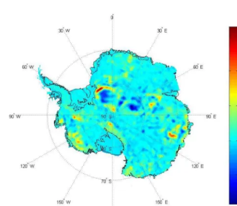
For our study, we computed a regular 0.25◦×0.25◦spatial grid of free air gravity anomalies over the Antarctica con-tinent with the DIR5 model, which is displayed in Fig. 1. The gravity anomalies have amplitudes between−120 and 111 mGal (more statistical data are provided in Table 1).
In this paper we have also used the only GRACE and LAGEOS mean gravity field model, EIGEN-GRGS.RL02bis (Bruinsma et al., 2010). This gravity field model is also pro-vided in terms of spherical harmonics up to degree 160, i.e., 125 km of spatial resolution.
2.2 BEDMAP models
BEDMAP 2 products (Fretwell et al., 2013) consist of grids describing surface elevation, ice thickness, the seafloor and subglacial bed elevation of the Antarctic south of 60◦S. These products were made by incorporating all available geophysical data. More details on the Antarctica subglacial landscape are visible in these products than in the previous BEDMAP model (Lythe et al., 2001) and the improved data coverage reveals the full details of mountain ranges, valleys, basins and troughs. Each dataset is provided in Antarctic Po-lar Stereographic projection, with latitude of true scale 71◦S
(datum WGS84). All heights are in meters relative to mean sea level as defined by the EIGEN-GL04C geoid (Foerste et al., 2008). The ice thickness, bedrock and surface elevation grids are provided at uniform 1 km spacing.
Table 1.Statistical data for maps used in this study. The first three rows are in milligals (mGal), and the others are in kilometers (km). The∗ indicates the application of a 77 km low-pass filter.
Minimum Maximum Mean SD
GOCE Free Air Anomaly −120.0 111.7 −4.2 22.5 Gravity terrain effect* −371.3 291.5 −64.6 154.2 Bouguer anomaly* −242.8 373.4 60.4 149.2
Crust model
Our crust model 29.7 51.0 40.9 3.4 CRUST1.0 (Laske et al., 2013) 7.5 45.9 35.7 3.4 AN1 (An et al., 2015) 7.9 65.0 35.9 7.6
Difference between crust models
CRUST1.0–AN1 −26.0 19.0 −0.3 4.2 GOCE BEDMAP–BEDMAP 2 −3.7 12.2 1.3 1.2 GOCE–GRACE −7.6 7.3 0.0 0.9 GOCE–CRUST1.0 −4.5 29.0 1.2 1.9
Figure 1. Free air anomalies in milligals (mGal) from the GOCE DIR5 solution.
did not include GOCE data. With the aim of representing the same range of wavelengths as the gravimetric anoma-lies, we analyze the difference between the two ice thick-ness estimates after filtering to the maximum spatial resolu-tion of GOCE, in this study 77 km. We notice that this differ-ence is largest at short and medium wavelengths (see Fig. 2). The maximum is 1628 m, the minimum is −896 m and the mean difference is 19 m. The new BEDMAP 2 seems to im-prove the estimate of the ice thickness all over the continent. A more complete comparison between the two products is given by (Hirt, 2014).
We select the datasets between BEDMAP and BEDMAP 2 so that Antarctica models and gravity observations remain
Figure 2.Difference between ice thickness from BEDMAP 2 and BEDMAP (max: 1628 m, min:−896 m, mean: 19 m). This differ-ence is filtered to the maximum spatial resolution of GOCE (77 km) to represent the range of wavelengths that are significant in our study.
independent. Finally, in order to have a consistent bedrock to-pography, it is calculated as the difference between the most precise topography from BEDMAP 2 and the ice thickness from BEDMAP.
2.3 Crustal thickness models from seismology
seis-Figure 3.Difference between crustal models AN1 and CRUST 1.0 based on seismological data. Units are kilometers (km).
mic observations, crustal thickness is constrained by gravity observations using maps from the British Antarctic Survey (Gaby Laske, personal communication, 2017). Baranov and Morelli (2013), in a Moho depth map compiling geophysical data, pointed out disagreements with CRUST1.0. The new version of this crust model may solve the problem.
Recently, another crustal model has been proposed by a Chinese team (An et al., 2015). This model is based exclu-sively on seismic observations. This will provide us with an independent model for comparison with our result from grav-ity data. In Antarctica, there are very few seismological ob-servations compared to gravity data, for example in areas of East Antarctica such as QML (Queen Maud Land) and AGV (George V Land; see the station distribution in Kanao et al., 2013, Fig. 1 or in An et al., 2015, Fig. 4). The comparison between the AN1 and CRUST1.0 models reveals large dif-ferences. As seen in Fig. 3, from−26 to+19 km, AN1 has higher values, mainly localized in the East Antarctic craton. West Antarctica is much thinner in CRUST1.0 than in the AN1 model. The roughness in the AN1 model around the coastline is related to its resolution. Including gravimetric observations (land and/or satellite) as constraints of the seis-mological model allows us to improve the spatial resolution.
3 Direct problem: terrain gravity effects
In order to estimate the gravity anomalies mainly due to crustal thickness variations, we compute, with Parker’s method (Parker, 1973), the gravitational terrain effects us-ing BEDMAP ice thickness, and BEDMAP 2 sea depth and surface topography. In our case, Parker’s approach is the most adequate because of the improved spatial resolution
ob-tained using GOCE observations. When the spatial resolu-tion is larger than 300 km, we cannot use a simple Bouguer approach to estimate gravity effects. Parker proposed using Fourier transforms to calculate the gravitational effect of an uneven, nonuniform layer of material.
To simplify the computations, the rock equivalent topog-raphy is calculated as (Balmino et al., 2012; Hirt, 2014) Hr=Hb+
ρo ρr
Ho+ ρi ρr
Hi, (1)
whereHris the rock equivalent topography,Hbthe bedrock topography,Hothe ocean depth,Hithe ice thickness,ρrthe rock density (2.670),ρothe sea water density (1.03) andρi the ice density (0.917).
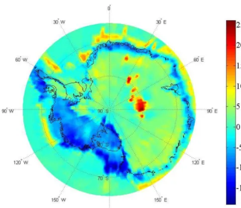
Using Parker’s method in a MATLAB function de-veloped by Simons (http://geoweb.princeton.edu/people/ simons/software.html, last access: 25 August 2015), we esti-mate the terrain gravitational effects by considering only one interface of constant densityρrwith a topography given by Eq. (1). The resulting gravitational effect filtered to GOCE spatial resolution on the pole (i.e., around 77 km) is shown in Fig. 4a.
The difference between the free air anomalies derived from GOCE and the terrain effects gives the Bouguer anomaly (Fig. 4b), which is essentially due to crustal thick-ness variations. However, the anomaly also includes the ef-fect of the errors in layer thickness given by the BEDMAP and BEDMAP 2 models, especially at long spatial wave-lengths, so that geophysical signal from the upper mantle may not be revealed by this study.
The statistical information on GOCE free air anomalies, gravitational terrain effects and Bouguer anomalies is given in Table 1. The free air gravity anomalies obtained by GOCE show variations between−120 and 110 mGal. The Bouguer anomalies vary between−250 and 360 mGal, with a very dif-ferent pattern. In Fig. 4b, there is a large discrepancy between the eastern part and the western part of the continent, which reflects the geological structure and history of Antarctica. There are also a lot of details at higher resolution revealed by the low degrees of spherical harmonics in the GOCE gravity field. The inversion of these Bouguer anomalies will help us better understand the crustal structure.
4 Inverse problem: crustal thickness estimation To obtain crustal thickness variations from our estimated Bouguer anomalies, we resolve the inverse problem using the Parker–Oldenburg iterative algorithm. For this purpose we use the 3dinver MATLAB function proposed by Gómez-Ortiz and Agarwal (2005), which allows for the computa-tion of a 3-D topography of a constant density layer to fit the Bouguer anomaly.
Figure 4. (a)Gravitational terrain effect derived from BEDMAP ice thickness, sea and bedrock topography. A low-pass filter of 77 km cutoff is applied.(b)Bouguer anomalies estimated as the difference between GOCE observed free air anomalies and terrain effects (in mGal).
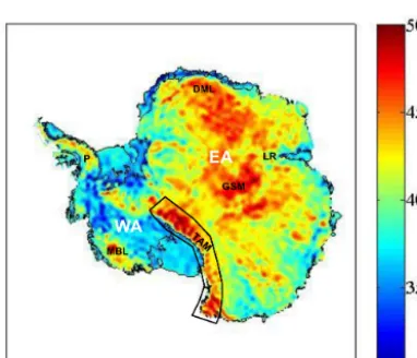
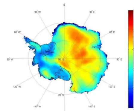
Figure 5. Estimation of crustal thickness (in km) from GOCE gravity observations. Geographical locations mentioned in the text are Dronning Maud Land (DML), Lambert Rift (LR), Gamburtsev Subglacial Mountains (GSMs), Transantarctic Mountains (TAMs), Marie Byrd Land (MBL) and the peninsula (P). The large TAMs separate East Antarctica (EA) from West Antarctica (WA).
as input the density contrast and the mean depth of the layer. Considering that the mantle density is 3.3, we choose a den-sity contrast of 0.63 to be consistent with our gravity terrain effects computation (rock density 2.670). According to pre-vious studies (Block et al., 2009; Ritzwoller et al., 2001), the mean Moho depth is about 40 km in West Antarctica and about 30 km in East Antarctica. We choose the average value, 35 km, as the mean depth for the whole continent for the starting computation.
A higher-cut filter is required to ensure convergence of the inverse problem (see Sect. 2; Gómez-Ortiz and Agarwal, 2005). In our case this filter restricts frequency contents be-tween wavelengths of 77 and 100 km.
Additionally, in order to provide information about the ac-curacy of the inversion, the 3dinver program computes the residual between the gravity effect of the output layer
topog-raphy and the observed Bouguer anomalies used as input. The RMS is only about 5 mGal, indicating a satisfactory fit.
The computed crustal thickness is shown in Fig. 5. Spatial variations from 29.7 to 51 km can be observed, with a mean thickness value of 41 km (see Table 1). The latter is slightly larger than the mean value of both seismological models be-cause for these models we included some thin oceanic crust in the estimation of the mean thickness. The AN1 model has a higher standard deviation compared to the others. This may come from the high noise level observed in a few geographi-cal areas.
(GSMs) seems to be independent from the surrounding ge-ological pattern. As the origin of these subglacial mountains was poorly known, a specific seismic survey was performed (Wolovick et al., 2009). With our regional map derived from GOCE data, it is now possible to follow specific geological structures over the whole continent. Our results can also be useful to develop and analyze an isostatic model to further interpret the topographic structures (O’Donnell and Nyblade, 2014).
5 Discussion
5.1 About our choices in the computation of the crustal model
5.1.1 BEDMAP or BEDMAP 2
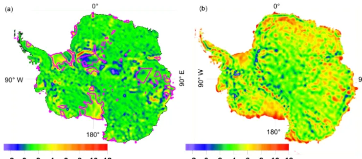
When computing the direct gravitational effect, we had to choose a model for all contributing layers. The best grids for the ice thickness and for the bedrock elevation are provided by BEDMAP in the most complete data compilation avail-able. The new version of these products, BEDMAP 2, also includes (satellite gravity) data from GRACE and GOCE. So we preferred to use the prior version BEDMAP for the ice thickness variations to have strictly independent grids, which allows us to estimate the gravitational effect of the ice. But BEDMAP 2 incorporates 2 orders of magnitude more data than BEDMAP, and it has a better spatial resolution, cover-age and precision at any wavelength. It is interesting to es-timate the impact of BEDMAP 2 in our crustal inversion. We did the same process as the previous calculation up to the computation of the crustal thickness, but using ice thick-ness from BEDMAP 2. The differences between the two so-lutions span from−3.7 to+12.2 km, but the standard devia-tion is only 1.2 km (see Table 1 for these statistical data). The higher values are not always located in the areas completed by satellite gravity in BEDMAP 2 because the large set of new data included during the computation really improved the model. In Fig. 6a, the pink line shows the areas for which no ground data were available within at least 50 km. We can trust that the new version of BEDMAP is closer to reality outside the pink line limit, and our direct estimation is more accurate within this limit. Some geological details appear in the crust variation estimate when computed with BEDMAP 2 ice thickness. The improvement of this version is important, even when dealing with the base of the continental crust. It would be interesting to have a version of this product that does not depend on satellite gravity data.
5.1.2 Improvement from GOCE compared to GRACE observations
GOCE is the latest of three space missions dedicated to grav-ity field modeling. In a lower-altitude orbit and equipped with a gradiometer, it measured smaller details of the gravity
field. The GRACE mission was launched at a higher altitude, mainly to observe temporal variations. But thanks to its long and still ongoing mission, it is also possible to compute an accurate geoid. The spatial resolution in the GRACE-derived geoid is less than that in the geoid obtained with GOCE, but we could evaluate the differences in our crust estimate using one or the other. Additionally, we hoped to see crustal details in the 77–120 km wavelength band. It should be noted that the GOCE geoid grid is a combined solution incorporating GRACE data.
The difference between the two crustal thicknesses, from only the GRACE model EIGEN-GRGS.RL02bis and from the GOCE DIR5 gravity anomalies, clearly shows a high-frequency signal corresponding to the contribution of GOCE at small spatial scales. The discrepancies are approximately ±7 km, emerging from the ambient noise level. They are mainly located over the Transantarctic Mountains (TAMs), the peninsula (P) and in the western part of the continent. In East Antarctica (EA), both models are really close. The differences do not exceed 2 km, except in the Lambert Rift (LR); see Fig. 5 for the location of the TAMs, P, EA and LR. The new GOCE DIR5 version thus provides interest-ing details for geological interpretation and knowledge of the Antarctic structure.
5.2 Comparison with models using seismology observations
5.2.1 The entire maps
We already compared both models issued from the seismol-ogy community (see Sect. 2.3). Clearly, CRUST1.0 appears to be closer to our result. We computed the difference be-tween them and plotted the corresponding map (Fig. 6b). Doing the same with the AN1 model will give differences identical to those between CRUST1.0 and AN1 because they dominate: the latter model is far from the two others.
The crustal thickness computed in this paper is on aver-age 1.2 km higher than for the CRUST1.0 model. The larger discrepancies are located all around the Antarctica continent because the two coast limits can differ. We also note that our crust estimate is thinner in the Transantarctic Mountains, in some regions of West Antarctica and in the center of East Antarctica. CRUST1.0 has smaller amplitude variations, and the lowest and highest values are reached by our model (see Table 1 for statistical results).
5.2.2 Spatial analysis of crustal models Spectral study
thick-Figure 6. (a)Differences between estimations of crustal thickness: results using BEDMAP minus results using BEDMAP 2. The pink line delimitates the zones where GOCE observations are used in BEDMAP 2. Units are kilometers (km).(b) Differences between the crust thicknesses computed from GOCE and the CRUST1.0 model. Units are kilometers (km).
ness from the GOCE DIR5 model and the one from only the GRACE EIGEN-GRGS.RL02bis model. This confirms the remark made in Sect. 5.1.2 about their very small spatial differences. Because the GOCE DIR5 grids also incorporate GRACE data, they are naturally close to one another, except when looking at wavelengths smaller than 120 km for which the differences are larger. The additional improvement by us-ing GOCE data at small wavelengths is not really clear.
The comparison of gravity-derived and seismological models shows a clear discrepancy between them even if the large-scale tendency is the same. The spectral densities show more energy for crustal thickness derived from gravity obser-vations (Fig. 7a).
In fact, we worked with the complete gravitational signal to invert the crustal thickness. This signal includes effects from the underlying mantle, which are not taken into ac-count in our interpretation. These effects likely have a long-wavelength pattern, but there is no specific signal in the spec-tral curve. Seismological models are not affected by these ef-fects and they share the same behavior at short wavelengths. Therefore, there is probably no significant mantellic distur-bance in our crustal thickness estimate. It is not possible to isolate and correct it during the computation process. Profile tracking
To compare the crustal models more easily, four profiles have been extracted along geographical paths (Fig. 7b) oriented S–N (c), W–E (d), NW–SE (e) and SW–NE (f). Firstly, the main differences appear over the oceans and over the two ice shelves because our inversion method is not adapted to these regions (we cut a part of the plots in Fig. 7). Secondly, there are large discrepancies near the coast limit, which are not the same for all models.
On the continent, CRUST1.0 is very close to our results, but it always has smaller thickness values. But as we had to
choose a mean depth to compute the Moho spatial variations, this difference is not relevant. Looking at the four plots, we see a higher discrepancy in the north and west parts of the continent. For example, in Dronning Maud Land, CRUST1.0 gives a thinner crust than our models. Smaller-scale varia-tions are visible in the GOCE DIR5 and GRACE EIGEN-GRGS.RL02bis profiles, while CRUST1.0 is smoother.
Clearly, AN1 is very different from the three others. It shows less spatial details, with a more constant profile along West Antarctica. In the Gamburtsev Subglacial Mountains region, the model reaches its maximum with a sudden thick-ening up to 65 km over a very restrictive area (Fig. 7d). No other model shows such a local crustal thickening.
Comparison with seismic receiver functions
To complete our work with seismic crustal thicknesses, we compare our results to those from receiver functions. We use the Antarctic Moho compilation given by An (Fig. 4 and Ta-ble S1 from An et al., 2015), who selected a list of stations to evaluate the quality of Moho depth (more details and sources can be found in An et al., 2015). In Fig. 8, we plot the dif-ferences between the crustal thickness from GOCE and the value derived from receiver functions. Roughly, we obtain the same discrepancies as those observed with the profiles in Fig. 7. There is a disagreement near the Gamburtsev Sub-glacial Mountains (GSMs) region. Seismic data show a thick-ening up to 60–65 km in this region, while gravity suggests a more regular crust with thicknesses under 50 km.
Figure 7.Spectral analysis crust thickness models(a)and their thickness variations over four profiles (shown with yellow lines in panelb). The Antarctica map is converted in a cartesianx−ycoordinate system. The profiles are(c)parallel toy,(d)parallel tox,(e)x=yand
Figure 8.Differences between crustal thicknesses obtained in this study and those from the compilation of receiver functions selected by An et al. (2015). Units are kilometers (km).
full crustal isostatic compensation of topography. In regions with mantle compensation or with density variations, our re-sults will differ from the real crustal thickness. Specific stud-ies have to be performed in regions where these effects are suspected based on seismic data but also on airborne (Schein-ert et al., 2016) or ground gravity data, the latter having a better resolution appropriate for local studies.
5.2.3 Density estimation
In our computation, we chose a 0.63 density contrast because it was consistent with previous studies and is a very classi-cal choice in such a geologiclassi-cal context. Recently, O’Donnell and Nyblade (2014) proposed a smaller contrast of 0.3 when they adjusted the crustal thickness based on gravimetric data to seismological results. Therefore, it was important to recon-sider the density of the crust and the upper mantle in Antarc-tica. We decided to use a simple Bouguer formula to estimate the density contrast variations, assuming that the observed Bouguer anomalies are mainly due to density variations. The Bouguer anomaly map is filtered to 333 km, and we chose the CRUST1.0 model for the crustal thickness. The result is shown in Fig. 9 and represents the variations around the crust’s mean density value of 2.67 when mantle density is fixed at 3.3. We notice that the density is slightly smaller in the western part of the continent. Few spatial variations are visible in Fig. 9. Density seems to be constant enough, from 2.72 to 2.8 in East Antarctica and from 2.62 to 2.75 in West Antarctica. Geological studies in this latter region indicate a complex assembly made up of several tectonic plates that are thinner and younger than the old eastern craton, explaining the density discrepancy. This is consistent with the results of Tenzer and Bagherbandi (2013), except in Marie Byrd Land where we found an increase in density not visible in their
Figure 9.Density variations estimated from CRUST 1.0 crustal thickness variations.
study. However, gravimetric observations do not need spa-tially varying density to be interpreted. A constant density contrast is a good first hypothesis to compute the inversion of the Bouguer anomalies and obtain the crustal thickness.
6 Conclusions
We provide a regional map of crustal thickness covering the entire Antarctic continent. Thanks to the new GOCE grav-ity field model, a spatial resolution of 77 km is reached with almost the same accuracy anywhere. Compared to previous studies, smaller details appear on the map, and the noise level is lower because we used the latest available gravity grids that compile all GRACE and GOCE data. However, the ice thickness estimation remains a key parameter during the pro-cess. An improved ice thickness map, made from radar satel-lite observations and fully independent from gravity data, would benefit not only glaciological but also our crustal stud-ies.
Currently, comparing our result to seismological models shows a fairly good agreement. Some studies already tried to use seismic observations to constrain the thickness derived from gravimetry, and seismological models are beginning to include gravimetric observations. A joint inversion of seis-mological and gravimetric data, including data from satellite missions, will provide the next crustal model of Antarctica.
Data availability. Our computed crustal thickness models of Antarctica will be available on the International Gravimetric Bu-reau website from 1 May 2018. (http://bgi.omp.obs-mip.fr/).
Competing interests. The authors declare that they have no conflict of interest.
Acknowledgements. We thank Gaby Laske for the information she provided to us about the CRUST1.0 model. We thank Anne Briais, who made very useful suggestions, and the reviewers for their con-structive comments. This work has been supported by University Paul Sabatier (Observatoire Midi-Pyrénées) and the French space agency CNES.
Edited by: Simon McClusky
Reviewed by: Meijan An and Duncan Young
References
An, M., Wiens, D. A., Zhao, Y., Feng, M., Nyblade, A. A., Kanao, M., Li, Y., Maggi, A., and Leveque, J.-J.: S-velocity model and inferred Moho topography beneath the Antarctic Plate from Rayleigh waves, J. Geophys. Res.-Sol. Ea., 120, 359–383, https://doi.org/10.1002/2014JB011332, 2015.
Balmino, G., Vales, N., Bonvalot, S., and Briais, A.: Spherical harmonic modelling to ultra-high degree of Bouguer and isostatic anomalies, J. Geod., 86, 499–520, https://doi.org/10.1007/s00190-011-0533-4, 2012.
Baranov, A. and Morelli, A.: The Moho depth map of the Antarctica region, Tectonophysics, 609, 299–313, 2013.
Bayer, B., Geissler, W. H., Eckstaller, A., and Jokat, W.: Seismic imaging of the crust beneath Dronning Maud Land, East Antarc-tica., Geophys. J. Int., 178, 860, https://doi.org/10.1111/j.1365-246X.2009.04196.x, 2009.
Block, A. E., Bell, R. E., and Studinger, M.: Antarctic crustal thick-ness from satellite gravity: Implications for the Transantarctic and Gamburtsev Subglacial Mountains, Earth Planet. Sc. Lett., 288, 194–203, https://doi.org/10.1016/j.epsl.2009.09.022, 2009. Bruinsma, S., Lemoine, J.-M., Biancale, R., and Valès, N.: CNES/GRGS 10-day gravity field models (Release 2) and their evaluation, Adv. Space Res., 45, 587–601, https://doi.org/10.1016/j.asr.2009.10.012, 2010.
Bruinsma, S. L., Förste, C., Abrikosov, O., Lemoine, J.-M., Marty, J.-C., Mulet, S., Rio, M.-H., and Bonvalot, S.: ESA’s satellite-only gravity field model via the direct approach based on all GOCE data, Geophys. Res. Lett., 41, 7508–7514, https://doi.org/10.1002/2014GL062045, 2014.
Chaput, J., Aster, R. C., Huerta, A., Sun, X., Lloyd, A., Wiens, D., Nyblade, A., Anandakrishnan, S., Winberry, J. P., and Wilson, T.: The crustal thickness of West Antarctica, J. Geophys. Res., 119, 378–395, https://doi.org/10.1002/2013JB010642, 2013. Dasgupta, S., Sengupta, S., Bose, S., Fukuoka, M., and Dasgupta,
S.: Polymetamorphism in the Schirmacher Hills Granulites, East Antarctica: Implications for Tectonothermal Reworking of an Isobarically Cooled Deep Continental Crust, Gondwana Res., 4, 337, https://doi.org/10.1016/S1342-937X(05)70334-8, 2001.
Drinkwater, M., Floberghagen, R., Haagmans, R., Muzi, D., and Popescu, A.: GOCE: ESA’s first Earth Ex-plorer Core mission, Space Sci. Rev., 108, 419–432, https://doi.org/10.1023/A:1026104216284, 2003.
Flament, T. and Rémy, F.: Dynamic thinning of Antarctic glaciers from along-track repeat radar altimetry, J. Glaciol., 58, 830–840, https://doi.org/10.3189/2012JoG11J118, 2012.
Foerste, C., Schmidt, R., Stubenvoll, R., Flechtner, F., Meyer, U., Koenig, R., Neumayer, H., Biancale, R., Lemoine, J.-M., Bru-insma, S., Loyer, S., Barthelmes, F., and Esselborn, S.: The Geo-ForschungsZentrum Potsdam/Groupe de Recherche de Geode-sie Spatiale satellite-only and combined gravity field models: EIGEN-GL04S1 and EIGEN-GL04C, J. Geod., 82, 331–346, https://doi.org/10.1007/s00190-007-0183-8, 2008.
Fretwell, P., Pritchard, H. D., Vaughan, D. G., Bamber, J. L., Bar-rand, N. E., Bell, R., Bianchi, C., Bingham, R. G., Blanken-ship, D. D., Casassa, G., Catania, G., Callens, D., Conway, H., Cook, A. J., Corr, H. F. J., Damaske, D., Damm, V., Ferracci-oli, F., Forsberg, R., Fujita, S., Gim, Y., Gogineni, P., Griggs, J. A., Hindmarsh, R. C. A., Holmlund, P., Holt, J. W., Jacobel, R. W., Jenkins, A., Jokat, W., Jordan, T., King, E. C., Kohler, J., Krabill, W., Riger-Kusk, M., Langley, K. A., Leitchenkov, G., Leuschen, C., Luyendyk, B. P., Matsuoka, K., Mouginot, J., Nitsche, F. O., Nogi, Y., Nost, O. A., Popov, S. V., Rignot, E., Rippin, D. M., Rivera, A., Roberts, J., Ross, N., Siegert, M. J., Smith, A. M., Steinhage, D., Studinger, M., Sun, B., Tinto, B. K., Welch, B. C., Wilson, D., Young, D. A., Xiangbin, C., and Zirizzotti, A.: Bedmap2: improved ice bed, surface and thickness datasets for Antarctica, The Cryosphere, 7, 375–393, https://doi.org/10.5194/tc-7-375-2013, 2013.
Gómez-Ortiz, D. and Agarwal, B. N. P.: 3DINVER.M: a MATLAB program to invert the gravity anomaly over a 3D horizontal density interface by Parker– Oldenburg’s algorithm, Comput. Geosci., 31, 513–520, https://doi.org/10.1016/j.cageo.2004.11.004, 2005.
Heeszel, D. S., Wiens, D. A., Anandakrishnan, S., Aster, R. C., Dalziel, I. W. D., Huerta, A. D., Nyblade, A. A., Wilson, T. J., and Winberry, J. P.: Upper mantle structure of central and West Antarctica from array analysis of Rayleigh wave phase velocities, J. Geophys. Res.-Sol. Ea., 121, 1758–1775, https://doi.org/10.1002/2015JB012616, 2016.
Helm, V., Humbert, A., and Miller, H.: Elevation and elevation change of Greenland and Antarctica derived from CryoSat-2, The Cryosphere, 8, 1539–1559, https://doi.org/10.5194/tc-8-1539-2014, 2014.
Hirt, C.: GOCE’s view below the ice of Antarctica: Satel-lite gravimetry confirms improvements in Bedmap2 bedrock knowledge, Geophys. Res. Lett., 41, 5021–5028, https://doi.org/10.1002/2014GL060636, 2014.
Jacob, T., Wahr, J., Pfeffer, W. T., and Swenson, S.: Recent con-tributions of glaciers and ice caps to sea level rise, Nature, 482, 514–518, https://doi.org/10.1038/nature10847, 2012.
Kanao, M., Yamada, A., and Toyokuni, G.: Passive Seismic De-ployments from the Lützow-Holm Bay to Inland Plateau of East Antarctica: The Japanese IPY Contribution to Structure and Seismicity, International Journal of Geosciences, 4, 837–843, https://doi.org/10.4236/ijg.2013.45077, 2013.
Landerer, F. W. and Swenson, S. C.: Accuracy of scaled GRACE terrestrial water storage estimates, Water Resour. Res., 48, W04531, https://doi.org/10.1029/2011WR011453, 2012. Laske, G., Masters, G., Ma, Z., and Pasyanos, M.: Update on
CRUST1.0 – A 1-degree Global Model of Earth’s Crust, Geo-phys. Res. Abstr., EGU2013-2658, EGU General Assembly 2013, Vienna, Austria, 2013.
Lemoine, M., Bruinsma, S., Loyer, S., Biancale, R., Marty, J.-C., Perosanz, F., and Balmino, G.: Temporal gravity field models inferred from GRACE data, J. Adv. Space Res., 39, 1620–1629, https://doi.org/10.1016/j.asr.2007.03.062, 2007.
Lindow, J., Kamp, P. J. J., Mukasa, S. B., Kleber, M., and Lisker, F.: Exhumation history along the eastern Amundsen Sea coast, West Antarctica, revealed by low temperature thermochronology, Tec-tonics, 35, 2239–2257, https://doi.org/10.1002/2016TC004236, 2016.
Llubes, M., Florsch, N., Legresy, B., Lemoine, J.-M., Loyer, S., Crossley, D., and Rémy, F.: Crustal thickness in Antarctica from CHAMP gravimetry, Earth Planet. Sc. Lett., 212, 103–117, https://doi.org/10.1016/S0012-821X(03)00245-0, 2003. Llubes, M., Lemoine, J.-M., and Rémy, F.: Antarctica seasonal mass
variations detected by GRACE, Earth Planet. Sc. Lett., 260, 127– 136, https://doi.org/10.1016/j.epsl.2007.05.022, 2007.
Lythe, M., Vaughan, D., and Consortium, B.: BEDMAP: A new ice thickness and subglacial topographic model of Antarctica, J. Geophys. Res.-Sol. Ea., 106, 11335–11351, https://doi.org/10.1029/2000JB900449, 2001.
McMillan, M., Shepherd, A., Sundal, A., Briggs, K., Muir, A., Ridout, A., Hogg, A., and Wingham, D.: Increased ice losses from Antarctica detected by CryoSat-2, Geophys. Res. Lett., 41, 3899–3905, https://doi.org/10.1002/2014GL060111, 2014. Memin, A., Flament, T., Remy, F., and Llubes, M.:
Snow-and ice-height change in Antarctica from satellite gravime-try and altimegravime-try data, Earth Planet. Sc. Lett., 404, 344–353, https://doi.org/10.1016/j.epsl.2014.08.008, 2014.
Mikhal’sky, E. V.: Main stages and geodynamic regimes of the Earth’s crust formation in East Antarcica in the Proterozoic and early Paleozoic, Geotectonics+, 42, 413–429, 2008.
O’Donnell, J. P. and Nyblade, A. A.: Antarctica’s hypsometry and crustal thickness: Implications for the origin of anomalous topog-raphy in East Antarctica, Earth Planet. Sc. Lett., 388, 143–155, https://doi.org/10.1016/j.epsl.2013.11.051, 2014.
Paech, H.-J. : Pervasive Pan-African reactivation of the Grenvil-lian crust and large igneous intrusions in central Dronning Maud Land, East Antarctica, Geol. Soc., 184, 343–355, 2001. Parker, R. L.: The Rapid Calculation of Potential
Anoma-lies, Geophys. J. R. Astron. Soc., 31, 447–455, https://doi.org/10.1111/j.1365-246X.1973.tb06513.x, 1973. Peng, P., Zhu, Y., Zhong, M., Kang, K., Du, Z., and
Yan, H.: Ice Mass Variation in Antarctica from GRACE Over 2002–2011, Mar. Geod., 39, 178–194, https://doi.org/10.1080/01490419.2016.1145609, 2016. Ramillien, G., Lombard, A., Cazenave, A., Ivins, E. R., Llubes,
M., Remy, F., and Biancale, R.: Interannual variations of
the mass balance of the Antarctica and Greenland ice sheets from GRACE, Global Planet. Change, 53, 198–208, https://doi.org/10.1016/j.gloplacha.2006.06.003, 2006.
Rémy, F. and Parouty, S.: Antarctic ice sheet and radar altimetry?: a review, Remote Sens., 1, 1212–1229, https://doi.org/10.3390/rs1041212, 2009.
Ritz, C., Rommelaere, V., and Dumas, C.: Modeling the evolution of Antarctic ice sheet over the last 420,000 years: Implications for altitude changes in the Vostok region, J. Geophys. Res., 106, 31 943–31 964, 2001.
Ritzwoller, M. H., Shapiro, N. M., Levshin, A. L., and Leahy, G. M.: Crustal and upper mantle structure beneath Antarctica and sur-rounding oceans, J. Geophys. Res.-Sol Ea., 106, 30 645–30 670, https://doi.org/10.1029/2001JB000179, 2001.
Scheinert, M., Ferraccioli, F., Schwabe, J., Bell, R., Studinger, M., Damaske, D., Jokat, W., Aleshkova, N., Jordan, T., Leitchenkov, G., Blankenship, D. D., Damiani, T. M., Young, D., Cochran, J. R., and Richter, T. D.: New Antarctic Grav-ity Anomaly Grid for Enhanced Geodetic and Geophysi-cal Studies in Antarctica, Geophys. Res. Lett., 43, 600–610, https://doi.org/10.1002/2015GL067439, 2016.
Simons, F. J.: Free software from the Simons Laborato-ries, available at: http://geoweb.princeton.edu/people/simons/ software.html (last access: 25 August 2015), 2018.
Tenzer, R. and Bagherbandi, M.: Reference crust-mantle density contrast beneath Antarctica based on the Vening Meinesz-Moritz isostatic inverse problem and CRUST2.0 seismic model, Earth Sci. Res. J., 17, 7–12, 2013.
Verron, J., Sengenes, P., Lambin, J., Noubel, J., Steunou, N., Guillot, A., Picot, N., Coutin-Faye, S., Sharma, R., Gairola, R. M., Murthy, D. V. A. R., Richman, J. G., Griffin, D., Pascual, A., Rémy, F., and Gupta, P. K.: The SARAL/AltiKa Altimetry Satellite Mission., Mar. Geod., 38, 2– 21, https://doi.org/10.1080/01490419.2014.1000471, 2015. Williams, S. D. P., Moore, P., King, M. A., and Whitehouse, P. L.:
Revisiting GRACE Antarctic ice mass trends and accelerations considering autocorrelation, Earth Planet. Sc. Lett., 385, 12–21, https://doi.org/10.1016/j.epsl.2013.10.016, 2014.
Wolovick, M., Block, A. E., Bell, R. E., Studinger, M., Ferrac-cioli, F., Braaten, D. A., and Damaske, D.: Preliminary analy-sis of the Gamburtsev subglacial mountains morphology from AGAP airborne radar data, EOS Trans AGU Fall Meet. Suppl., 90, available at: http://search.ebscohost.com/login.aspx?direct= true&site=eds-live&db=geh&AN=2016-019425 (last access: 31 July 2017), 2009.
Zwally, H. J., Schutz, B., Abdalati, W., Abshire, J., Bentley, C., Brenner, A., Bufton, J., Dezio, J., Hancock, D., Hard-ing, D., HerrHard-ing, T., Minster, B., Quinn, K., Palm, S., Spin-hirne, J., and Thomas, R.: ICESat’s laser measurements of polar ice, atmosphere, ocean, and land, J. Geodyn., 34, 405, https://doi.org/10.1016/S0264-3707(02)00042-X, 2002. Zwally, H. J., Li, J., Brenner, A. C., Beckley, M., Cornejo, H. G.,