Large eddy simulation model for wind-driven sea circulation in coastal areas

(1)

Nonlin. Processes Geophys., 20, 1095–1112, 2013 www.nonlin-processes-geophys.net/20/1095/2013/ doi:10.5194/npg-20-1095-2013

Nonlinear Processes

in Geophysics

Open Access

Large eddy simulation model for wind-driven sea circulation in

coastal areas

A. Petronio1, F. Roman1, C. Nasello2, and V. Armenio1

1_{Dipartimento di Ingegneria e Architettura, Università di Trieste, Piazzale Europa 1, 34127 Trieste, Italy} 2_{Dipartimento di Ingegneria Civile, Ambientale e Aerospaziale, Università di Palermo, Viale delle Scienze,} 90128 Palermo, Italy

Correspondence to: V. Armenio ([email protected])

Received: 10 June 2013 – Revised: 5 November 2013 – Accepted: 6 November 2013 – Published: 10 December 2013

Abstract. In the present paper a state-of-the-art large eddy simulation model (LES-COAST), suited for the analysis of water circulation and mixing in closed or semi-closed areas, is presented and applied to the study of the hydrodynamic characteristics of the Muggia bay, the industrial harbor of the city of Trieste, Italy. The model solves the non-hydrostatic, unsteady Navier–Stokes equations, under the Boussinesq ap-proximation for temperature and salinity buoyancy effects, using a novel, two-eddy viscosity Smagorinsky model for the closure of the subgrid-scale momentum fluxes. The model employs: a simple and effective technique to take into ac-count wind-stress inhomogeneity related to the blocking ef-fect of emerged structures, which, in turn, can drive local-scale, short-term pollutant dispersion; a new nesting proce-dure to reconstruct instantaneous, turbulent velocity compo-nents, temperature and salinity at the open boundaries of the domain using data coming from large-scale circulation mod-els (LCM). Validation tests have shown that the model repro-duces field measurement satisfactorily. The analysis of wa-ter circulation and mixing in the Muggia bay has been car-ried out under three typical breeze conditions. Water circu-lation has been shown to behave as in typical semi-closed basins, with an upper layer moving along the wind direc-tion (apart from the anti-cyclonic veering associated with the Coriolis force) and a bottom layer, thicker and slower than the upper one, moving along the opposite direction. The study has shown that water vertical mixing in the bay is in-hibited by a large level of stable stratification, mainly associ-ated with vertical variation in salinity and, to a minor extent, with temperature variation along the water column. More in-tense mixing, quantified by sub-critical values of the gradient Richardson number, is present in near-coastal regions where

upwelling/downwelling phenomena occur. The analysis of instantaneous fields has detected the presence of large cross-sectional eddies spanning the whole water column and con-tributing to vertical mixing, associated with the presence of sub-surface horizontal turbulent structures. Analysis of water renewal within the bay shows that, under the typical breeze regimes considered in the study, the residence time of water in the bay is of the order of a few days. Finally, vertical eddy viscosity has been calculated and shown to vary by a couple of orders of magnitude along the water column, with larger values near the bottom surface where density stratification is smaller.

1 Introduction

Coastal basins are in general shallow and characterized by complex geometry arising from rapid varying bathymetry, coastline and anthropic structures. Such features may pro-duce three-dimensionality, breaking waves and along-shore currents. In semi-closed basins, wind shear stress is the main forcing term directly driving water surface layers and trigger-ing mechanical turbulence production. In such conditions, in-teraction with the coastline develops downwelling/upwelling along vertical planes and the inversion of the mean velocity field in the bottom layer of the water column with respect to the superficial one. The resulting additional shear enhances further mechanical turbulence production. Further, in coastal regions, variations in temperature and salinity along the wa-ter column give rise to buoyancy-driven mixing.

(2)

1096 A. Petronio et al.: LES model for wind-driven sea circulation in coastal areas

The aforementioned features make modeling of coastal hydrodynamics quite challenging for general circulation ocean models, which, on the other hand, have been conceived and calibrated for analysis of meso, or even larger, scales. Further, coastal hydrostatic or three-dimensional models de-veloped in the hydraulic engineering community, which make use of basic turbulence parametrization, are often not suited for detailed and accurate analysis of internal mixing in coastal areas. For example, it has been recognized that the hydrostatic approximation, adopted by most models, cannot be applied successfully for the coastal environment where upwelling/downwelling phenomena play an important role; moreover, most coastal models adopt the Reynolds-averaged (RANS) approach, which is not designed to reproduce the interplay between physical mechanisms occurring in coastal regions (see Burchard et al., 2008).

On the other hand, the increased computational capabil-ity available over the years has made possible new mod-eling approaches to the problem. In particular, large eddy simulation (LES) has recently emerged as a powerful and promising methodology to afford real-scale coastal prob-lems characterized by the occurrence of complex phys-ical processes in complex geometries (Burchard et al., 2008). In LES the large scales of motion, typically three-dimensional and anisotropic, are directly solved through a 3-D unsteady simulation, whereas the spatial scales of mo-tion whose dimensions are smaller than the grid spacing (sub-grid scales, SGS), more dissipative and isotropic, are parametrized through the use of a proper model.

Large eddy simulations for ocean applications were first carried out by Skyllingstad and Denbo (1995). The authors considered simple geometry (a Cartesian box) to study the dynamics of plumes under convective conditions. Other stud-ies have made use of LES for the analysis of mixing in the open ocean (see, among others, Wang et al., 1996). A review of the use of LES for marine application is in Scotti (2010).

As briefly described above, in coastal regions complica-tions arise, and properly designed numerical models must be used. A three-dimensional coastal basin exhibits horizontal and vertical length scales very different from each other. The horizontal one is of the order of a few kilometers, whereas the vertical one usually lies within the range of 10 to 100 m. Turbulence itself displays large horizontal structures that are ruled mostly by the Earth’s rotation and by the free surface and solid boundaries, giving rise to strongly anisotropic flow features. Unfortunately, in LES, eddy-viscosity SGS models are mostly designed for isotropic or nearly isotropic grids, making prohibitive mesh requirements for real-scale coastal studies (for a discussion see Scotti et al., 1993). In high-resolution LES of real-scale coastal hydrodynamics, grid res-olution in the horizontal direction can be pushed up to 10-to-1 m, whereas the vertical resolution may be of the order 0.5 m, introducing large anisotropy to the grid topology itself and, hence, to the implicit filter widths. When isotropic SGS models are used in the presence of large cell anisotropy, they

overestimate the contribution of the unresolved scales of mo-tion, producing over-dissipamo-tion, which strongly affects the accuracy of the simulation. Recently, Roman et al. (2009c) proposed an SGS model properly suited for coastal applica-tions, thus able to take into account the physics and the ge-ometric complexities usually encountered in real-case appli-cations. It implements a modified anisotropic Smagorinsky model (ASM) that takes advantage of the two-eddy-viscosity idea borrowed from geophysical fluid dynamics concepts. The model, applied to the analysis of water mixing and re-newal in Barcelona harbor (see Galea et al., 2012), has been shown to be able to reproduce correctly the velocity of the wind-induced current as well as the complex flow patterns developing within the harbor. The results corroborate the findings of Ramachandran et al. (2013) about the ability of LES used in conjunction with the ASM model to reproduce accurately flow features in coastal hydrodynamics.

However, additional issues are still to be addressed for the application of LES methodology to real-scale coastal stud-ies. The assessment of proper conditions at the boundaries of the computational domain has a relevant impact. From one side, the suitable assignment of momentum and heat fluxes at the free surface is of crucial importance for the accurate re-production of the wind-driven circulation at a coastal scale. Further, since the near-shore circulation is always affected by mesoscale circulations, proper procedures are required to nest the high-resolution LES simulation within large-scale circulation models.

To summarize, analysis of water dynamics in areas char-acterized by interplay of different physical processes and ge-ometrical complexities, like harbors and lakes, may take ad-vantage of novel state-of-the-art, properly designed, numeri-cal tools able to reproduce such features.

The scope of the present paper is to show a novel, state-of-the-art, numerical model suited for analysis of mixing and water renewal in coastal semi-closed regions (i.e., harbors) and lakes. The model solves the Boussinesq form of 3-D non-hydrostatic, primitive-variable, filtered Navier–Stokes equa-tions, considering temperature and salinity effects on buoy-ancy in the water column as well as dispersion of passive scalars (i.e., pollutants). The unresolved subgrid scales de-riving from the filtering operations are parametrized through a novel two-eddy viscosity Smagorinsky model. The model employs: (a) a simple and effective procedure to take into ac-count wind-stress inhomogeneity at a local scale, related to topographic effects in the low atmosphere or, among other things, to the presence of ships or jetties; (b) a novel nesting methodology combining interpolation procedure of the flow variable from the LCM domain to the LES one, together with a synthetic generation of turbulence within the LES domain, to reproduce realistic dynamics within the area of interest. Finally, the model is applied to the analysis of water circula-tion and mixing in the Muggia bay, a site of great interest in Italy from the water quality point of view, due to the presence of potentially dangerous industrial plants.

(3)

A. Petronio et al.: LES model for wind-driven sea circulation in coastal areas 1097

The paper is organized as follows: in Sect. 2 the numerical model (LES-COAST) is presented along with a detailed dis-cussion of the boundary conditions at the free-surface and at the open sections. In Sect. 3 the model is firstly vali-dated against field data, and successively water circulation and mixing in the Muggia bay are discussed. Finally, con-cluding remarks are given in Sect. 4.

2 Governing equations

LES-COAST solves the Boussinesq form of the filtered, 3-D, non-hydrostatic Navier–Stokes equations together with the transport equations for temperature and salinity. Transport of pollutants treated through an advection–diffusion equation for their concentrations (or as dispersed Lagrangian parti-cles) is also implemented in the model. The governing equa-tions read as:

∂uj

∂xj

=0 (1)

∂ui

∂t +

∂uiuj

∂xj

= −1

ρ0

∂p ∂xi

+ν ∂

2_u i

∂xj∂xj

−2ij kjuk+

−ρ

ρ0

giδi,2−

∂τij

∂xj (2)

∂T

∂t +

∂ujT

∂xj

=kT ∂

2_T

∂xj∂xj −∂λ

T j

∂xj

(3)

∂S

∂t +

∂ujS

∂xj

=kS ∂

2_S

∂xj∂xj −

∂λS_j

∂xj

(4)

∂Cn

∂t +

∂ujCn

∂xj

=kCn ∂

2_C n

∂xj∂xj −∂λ

Cn

j

∂xj

n=1,2,· · ·, (5) whereui,p,T, andSare, respectively, the velocity compo-nent in the xi direction, the hydrodynamic kinematic pres-sure, temperature (in Kelvin) and salinity (in PSU);gis the gravitational acceleration,itheith component of the Earth rotation vector, andρandρ0are density anomaly and its ref-erence value, respectively.ν,kT andkSare kinematic viscos-ity, and thermal and salinity diffusivviscos-ity, respectively. Since the density anomaly due to salinity and temperature vari-ations is much smaller than the bulk density of the water, in coastal applications the buoyancy force can be accounted for by the Boussinesq approximation through the equation of state:

ρ=ρtot−ρ0

ρ0

= −βT(T−T0)+βS(S−S0), (6) whereρtotis the total density,T0andS0are reference values giving the densityρ0, andβT andβS are expansion coeffi-cients for temperature and salinity, respectively.Cnin Eq. (5) refers to the concentration of thenth pollutant andkCnis its

kinematic diffusivity. Over-bar refers to the filtering opera-tion. LES-COAST uses an implicit filter, meaning that filter-ing is implicitly performed in the physical space through a top-hat filter function represented by the cell size. The latter term on the right-hand side of Eqs. (2)–(5) represents the sub-grid contributions to momentum and scalar fluxes, respec-tively. The sub-grid scale momentum fluxes are parametrized by the two-eddy-viscosity anisotropic Smagorinsky model (ASM) described in Roman et al. (2010) and briefly sum-marized hereafter.

In the standard Smagorinsky model, SGS stresses are ex-pressed as:

τSGS,ij= −2νtSij, (7)

whereSij is the resolved strain rate tensor

Sij= 1 2

_∂u i

∂xj +∂uj

∂xi

(8) andνt is SGS eddy viscosity.

The Smagorinsky model is isotropic and eddy viscosity is evaluated as the product of a length scale C1, propor-tional to the grid size, and a velocity scaleC1|S|, where

C is a constant and |S| is the contraction of the resolved strain rate tensor. In moderate-to-strong anisotropic grids it is difficult to define a single length scale. In particular, set-ting1=(1x1y1z)1/3leads to an excessive overestimation of the eddy viscosity in all directions. Thus, in Roman et al. (2010) a two eddy-viscosity model was developed, one for the horizontal direction and another for the vertical one, re-spectively. The two eddy viscosities are defined as:

νt,h=(ChLh)2|Sh|, (9)

νt,v=(CvLv)2|Sv|, (10)

where Lh=(12x+1z2)1/2 and Lv=1y are proper length scales for horizontal and vertical directions, respectively. The velocity scales in the horizontal and vertical directions are obtained through the following contractions of the strain rate tensor:

|Sh| = q

2S2₁₁+2S2₃₃+4S2₁₃ (11) |Sv| =

q

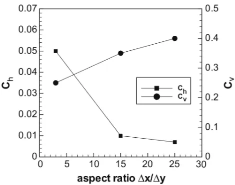
4S2₁₂+2S2₂₂+4S2₂₃. (12) The model contains two empirical constants,ChandCv, respectively, that need calibration. This has been carried out simulating the well-recognized, turbulent-plane Poiseuille flow (also referred to as plane channel flow) with increasing grid anisotropy, comparing first- and second-order statistics with reference experimental and numerical data (details are in Roman et al., 2010). In Fig. 1 we show the optimal coeffi-cients obtained in the calibration process.

Reynolds analogy is assumed to hold for scalars, setting

P rsgs=Scsgs=0.8.

(4)

1098 A. Petronio et al.: LES model for wind-driven sea circulation in coastal areas A. Petronio et al.: LES model for wind driven sea circulation in coastal areas 3

Fig. 1.Variation of optimal values constantsCh andCvwith the

grid anisotropy.

against field data and water circulation and mixing in the 175

Muggia bay is discussed. Finally, concluding remarks are given in Section 4.

2 Governing equations

LES-COAST solves the Boussinesq form of the filtered, 3D non-hydrostatic, Navier-Stokes equations together with 180

the transport equations for temperature and salinity,T and

S respectively. Transport of pollutants treated through an advection-diffusion equation for their concentrations (or as dispersed Lagrangian particles) is also implemented in the model. The governing equations read as:

185

∂uj ∂xj

= 0 (1)

∂ui ∂t +

∂uiuj ∂xj

=−1 ρ0

∂p ∂xi

+ν ∂

2_u

i ∂xj∂xj

−2Ωi×ui+

−ρ ρ0

giδi,2−∂τij

∂xj

(2)

190

∂T ∂t +

∂ujT ∂xj

=kT ∂

2_T

∂xj∂xj −∂λ

T j ∂xj

(3)

∂S ∂t +

∂ujS ∂xj

=kS ∂

2_S

∂xj∂xj −∂λ

S j ∂xj

(4)

∂Cn ∂t +

∂ujCn ∂xj

=kCn ∂ 2_C

n ∂xj∂xj

−∂λ Cn

j ∂xj

n= 1,2,· · · (5)

whereui,p,T, andS are respectively the velocity

compo-nent in thexi direction, the hydrodynamic kinematic

pres-195

sure, temperature (in Kelvin) and salinity (in PSU);gis the

gravitational acceleration,Ωithe i-th component of the Earth

rotation vector, ρ andρ0 are density anomaly and its

ref-erence value respectively.ν,kT _and_kS _{are kinematic}

vis-cosity, thermal and salinity diffusivity respectively. Since the 200

density anomaly due to salinity and temperature variations is much smaller than the bulk density of the water, in coastal applications the buoyancy force can be accounted for by the Boussinesq approximation through the equation of state:

ρ=ρT−ρ0 ρ0

=−βT(T−T0) +βS(S−S0) (6)

205

whereρT is the total density,T0andS0are reference values

giving the densityρ0,βT andβSare expansion coefficients

for temperature and salinity respectively.Cn in Equation 5

refers to the concentration of the n-th pollutant andkCn_{is its}

kinematic diffusivity. Over-bar refers to the filtering opera-210

tion. LES-COAST uses implicit filter, meaning that filtering is implicitly performed in the physical space through a top-hat filter function represented by the cell size. The latter term on the right hand side of Equations 2-5 represents the sub-grid contributions to momentum and scalar fluxes respec-215

tively. The sub-grid scale momentum fluxes are parametrized by the two-eddy-viscosity Anisotropic Smagorinsky Model (ASM) described in Roman et al. (2010) and briefly summa-rized hereafter.

In the standard Smagorinsky model, SGS stresses are ex-220

pressed as:

τSGS,ij=−2νtSij (7)

whereSij is the resolved strain rate tensor

Sij=

1 2

_∂u i ∂xj

+∂uj ∂xi

(8)

andνtis SGS eddy viscosity.

225

The Smagorinsky model is isotropic and eddy viscosity is evaluated as product of a length-scale C∆, proportional to the grid size, and a velocity scale C∆|S|, where C is a constant and |S|is the contraction of the resolved strain rate tensor. In moderate-to-strong anisotropic grids it is dif-230

ficult to define a single lengths-cale. In particular, setting

∆ = (∆x∆y∆z)1/3 leads to an excessive overestimation of

the eddy viscosity in all directions. Thus, in Roman et al. (2010) a two eddy-viscosity model was developed, one for the horizontal directions and another for the vertical one re-235

spectively. The two eddy viscosity are defined as:

νt,h= (ChLh)2|Sh| (9)

νt,v= (CvLv)2|Sv| (10)

whereLh= (∆2x+ ∆2z)1/2andLv= ∆y are proper

length-240

scales for horizontal and vertical direction respectively. The velocity scales in the horizontal and vertical directions are

Fig. 1. Variation in optimal value constants,ChandCv, with the grid anisotropy.

The complex geometry of the coastal hydrodynamic prob-lem is treated by a combination of a body-fitted curvilinear grid (Zang et al., 1994) and the immersed boundary method (IBM) recently developed by Roman et al. (2009b).

In IBM, the governing equations are solved over a reg-ular Cartesian or curvilinear, structured computational do-main; internal obstacles are reproduced through proper mod-ification of the governing equations at these special loca-tions. Among others, we use the direct forcing approach, meaning that a body force is added to the momentum equa-tions to mimic the presence of solid boundaries (see Fadlun et al., 2000 and the successive paper by Balaras (2004) for a description of the methodology in Cartesian coordinates). In Roman et al. (2009b) the method was improved and ex-tended to curvilinear-coordinate formulation of the Navier– Stokes equations. The advantage of IBM over unstructured mesh solvers is that particular care is not required to adapt the computational mesh to the domain shape, and complex ge-ometry can be treated in an easy and efficient way. Our strat-egy is to adopt curvilinear coordinates to shape the compu-tational domain over the physical one to minimize the num-ber of inactive computational cells. Immersed boundaries are used to reproduce geometric complexities such as coastlines and anthropic structures such as docks, jetties and breakwa-ters.

2.1 Boundary conditions over solid boundaries

In wall-bounded turbulence, LES can be performed ei-ther by solving the near-wall viscous sublayer or through parametrization of the near-wall effects on the inertial region of turbulence. The computational cost of LES resolving the near-wall viscous layer (wall-resolving LES) is proportional toRe2.5 (see Piomelli, 2008), limiting such a class of sim-ulations to low values of Re. Moreover, in wall-resolving

LES, it is not clear how to consider wall roughness explic-itly. The alternative strategy, consisting of skipping the so-lution of the near-wall layer through parametrization of the wall shear stress, allows the application of the methodology to full-scale values ofRe, also including the effect of wall roughness on the dynamics of the boundary layer. This is the strategy adopted in LES-COAST. Specifically, we use two different approaches, depending on whether the solid ary is body-fitted or reproduced by using immersed bound-aries.

For body-fitted solid boundaries the logarithmic law of the wall is used at the first node off the wall:

u+(1)=1

klog y

+

(1)+B, (13)

whereu+(1)denotes the tangential velocity at the first grid point off the wall, made non-dimensional with the friction velocityuτ,k=0.41 is the von Karman constant,y+(1)is the distance from the wall of the first computational mesh point, scaled with the viscous length scaleν/uτ, andB is a coefficient that also includes roughness effects. This equation is solved iteratively to determine the friction velocity used to compute the wall shear stress, which is employed as a bound-ary condition.

This technique can hardly be applied to solid walls re-produced using immersed boundaries, because in the gen-eral cases, cell faces do not coincide with immersed bound-aries. In order to overcome this issue, a novel approach has been proposed by Roman et al. (2009a). It consists of a two-step procedure: first the velocity at the first off-the-wall node (with respect to the immersed boundary) is calculated through Eq. (13) using the velocity field from the interior; second, a RANS-like eddy viscosity is set at the interface be-tween the fluid region and the solid one asνt=kuτy, where

yis the distance from the surface of the immersed boundary and the first fluid node. Details of the method are in Roman et al. (2009a).

2.2 Boundary conditions at the free surface

In LES-COAST, wind forcing over the free surface is taken into account by means of the formula proposed in Wu (1982), in which the induced stress at the sea surface,τ, is computed from the wind velocity 10 m above the mean sea levelU10 as:

C10 =(0.8+0.065U10)10−3 (14)

τ =ρC10U102, (15)

whereC10represents the drag coefficient. In the literature it is established that the kind of forcing at the free surface may play a role in the dynamics of the upper layer. Although in the literature better methods can be found, we use a zero-mean random fluctuation with 20 % variance, added to the referenceτ, to give a more realistic forcing action and, at the same time, to facilitate the generation of turbulence in the

(5)

A. Petronio et al.: LES model for wind-driven sea circulation in coastal areas 1099

Fig. 2. Schematic view of the recirculation zones of the wind flow around obstacles. Figure reproduced with modifications from Kuehn and

Coleman (2005).

upper layers. Since randomization acts over the shear-stress components, it implicitly acts on the stress angle as well. This method has proven to be reliable and able to trigger turbu-lence in a very efficient way. In particular, by analysis of the instantaneous velocity field, we found sub-surface coherent structures typically developing in wall-bounded (or interfa-cial) turbulence.

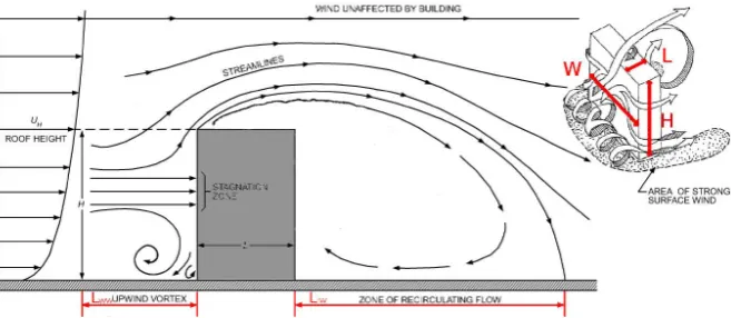
Close to obstacles such as docks, ships and breakwaters, the wind strays locally from the mean path and gives rise to complex recirculating patterns. Such local phenomena can play an important role in the surface layer dynamics at harbor scale. A detailed reproduction of such effects would come from a fully-coupled simulation of the low-atmosphere dy-namics together with water basin dydy-namics, with integrated boundary conditions able to conserve momentum and heat fluxes at the interface. Such an integrated model is not avail-able at the moment and, on the other hand, it would require a computational cost at least as large as twice that required for the marine basin simulation. Rather, we employ a simplified, computationally inexpensive, engineering approach that is currently in use in numerical simulations of short-range pol-lutant dispersion in the low atmosphere (Scire et al., 2000). Specifically, LES-COAST incorporates local effects into spa-tial distribution of the wind shear stress, taking advantage of some relevant literature formulations concerning studies on turbulent flow patterns around three-dimensional obstacles on a plane surface. Following Hosker (1984) and Hanna et al. (1982), we denote withHandW, respectively, the character-istic height of the obstacle and its own length perpendicular to the wind direction, and withLits characteristic width in the cross-wind direction (see the upper right panel of Fig. 2). The relationships between the aspect ratios of the obstacle and the extension of the recirculation region are discussed in detail in Hosker (1984). The authors suggest:

Llw= H

A (W/H )

1+B (W/H ) if

L

H ≤2, (16)

Llw=1.75H

(W/H )

1+0.25(W/H ) if L

H >2 (17)

for the leeward recirculation lengthLlw, where

A= −2+3.7

L H

−1/3

and

B= −0.15+0.305 _L

H

−1/3

.

The proposed formulas classify the obstacles into two cate-gories based on the ratio L

H. If L

H >2, the recirculation does

not depend on the width of the obstacle. The windward cav-ity length,Lww, is given in Hanna et al. (1982) and reads:

Lww=2H, (18)

regardless of other parameters. In the model the influence of the obstacles is considered through a linear damping of the wind stress along the recirculation pattern, from the reference value at distanceLlworLwwfrom the obstacle to zero at the solid boundary. In case of time-varying wind conditions, the model calculates successive damping-factor maps. A linear interpolation procedure computes the updated values in the intermediate steps between two consecutive maps.

2.3 Boundary conditions at open boundaries

Boundary conditions at the open sections of the domain are supplied by nesting LES-COAST within an LCM. The nest-ing methodology consists of two main steps: first we inter-polate LCM data (velocity components, turbulent kinetic en-ergy TKE, temperature, salinity and pollutant concentration,

(6)

11006 A. Petronio et al.: LES model for wind-driven sea circulation in coastal areasA. Petronio et al.: LES model for wind driven sea circulation in coastal areas

Fig. 3.Sketch of the channel flow case with the buffer sub-domain.

With indexes are denoted the sections used in the comparison.

if any) at the inflow/outflow (i/o) boundaries of the LES do-main. Since LCM simulations usually have larger time steps 400

than LES, linear interpolation between two successive LCM time steps data is performed for the intermediate LES time steps; second, we place a buffer sub-domain between the i/o boundaries and the interior LES domain, in which tur-bulence is triggered by means of a divergence-freesynthetic, 405

zero-mean, fluctuating body forceb′

i, added to the right-hand

side of momentum Equation 2. This allows to generate a divergence-free fluctuating field which can be superimposed to the incoming mean velocity field. In order to generate fluctuating velocity components representative of the turbu-410

lence level in the flow field, the intensity of the body force is automatically adjusted based on the mean velocity profiles,

URAN Si

1_{, and the}_{T KE}

RAN Scontent coming from the

in-terpolation procedure. The transport equation ofT KE equa-tion reads:

415

∂T KE

∂t =T R− hu

′

iu′ji ∂Ui ∂xj+hb

′

iu′ii −Φ (19)

where, withh.i, we denote an averaging operation. In Equa-tion 19 T Rrepresent transport terms, Φ is the dissipation rate ofT KE, the second term on the right hand side is me-chanical production ofT KEand the third one issynthetic

420

production of turbulence.

The production terms extract energy from the mean flow to feed the fluctuating counterpart. At the inlet, the mean veloc-ity component is provided from the LCM and the production term is zero. Therefore its role is taken by thesynthetic pro-425

duction termhb′

iu′ii.

At the first time step, in the buffer sub-domain, velocity fluctuations are absent, therefore the left hand side of Equa-tion 19 reduces to the target value for the turbulent kinetic energy (T KERAN S) divided by the time step. All terms of

430

the rhs are zero buthb′

iu′ii. The body-force can be constructed

1

Here with the indexRAN S_{we denote data coming from LCM} simulations based on the solution of the Reynolds Averaged Navier-Stokes equations A A A A A A A AA

AA A A AAA C C C C C C C CC

CC CC CCC

E E E E E E E EE

EE E E E EE

G G G G G G G GG

GG G GGGG I I I I I I I I I

II I I I II

K K K K K K K KK

K KK K KKK M M M M M M M MM

M MM M MMM O O O O O O O OO

O OO O OOO Q Q Q Q Q Q QQ

Q QQ Q QQQ S S S S S S SS

S SS S S SS U U U U U U UU

U UU U UUU W W W W WW WW

W WWW WWW y+ u / uτ 10000 20000 18 19 20 21 22 23 24 25 26 27 28 29 RANS/LES RANS/LES RANS/LES RANS/LES RANS/LES RANS/LES RANS/LES RANS/LES RANS/LES RANS/LES RANS/LES RANS/LES LES periodic channel A C E G I K M O Q S U W

Fig. 4.Comparison of the mean velocity profile for nested channel

flow simulation without body-force. Red dashed line: reference re-sults from the periodic channel simulation; black lines: mean veloc-ity profile at different sections of the channel with the buffer region.

in a discrete form as:

b′

i=

∆T KE u′

i∆t

= T KERAN S u′

i∆t

(20)

where, at the first time step, the velocity fluctuations are com-puted from the mean velocity profile as

435

u′i=ciURAN SiR (21)

being ci a coefficient and R a suitable zero meancolored noisefunction. After the first time step, the body-force gives rise to velocity fluctuations in the buffer sub-domain, the shear production term starts to extract energy from the mean 440

flow and the forcing term must adapt itself to the flow condi-tions. This is accomplished by the proper definition in Equa-tion 20 of the velocity scale, which is based on the actual fluctuation level in the flow: an increased value ofu′

i

corre-sponds to a decreased value ofb′

iand vice-versa. The velocity

445

fluctuations can be easily computed because the mean flow is known at the boundary.

In order to provide a smooth transition from the buffer sub-domain to the reference one, the forcing term is exponentially damped to a target value bT, which is zero, at the end of

450

the buffer region, subtracting to the functionbi(x)the term ef(x)₍_b

i(x)−bT(x)).

Validation tests have been performed for the turbulent

plane-channel flow case, at Reτ=uτδ/ν= 20000 (with

uτ= p

τw/ρthe friction velocity,τw the wall shear stress,

455

andδthe half height of the channel). It corresponds to a bulk Reynolds number of the order of106_{, (Pope, 2000, pp.279) ,}

Fig. 3. Sketch of the channel flow case with the buffer sub-domain.

The sections used in the comparison are denoted with indexes.

if any) at the inflow/outflow (i/o) boundaries of the LES do-main. Since LCM simulations usually have larger time steps than LES, linear interpolation between two successive LCM time steps data is performed for the intermediate LES time steps; second, we place a buffer sub-domain between the i/o boundaries and the interior LES domain, in which tur-bulence is triggered by means of a divergence-free synthetic, zero-mean, fluctuating body forceb0_i, added to the right-hand side of momentum Eq. (2). This allows one to generate a divergence-free fluctuating field that can be superimposed on the incoming mean velocity field. In order to generate fluctuating velocity components representative of the turbu-lence level in the flow field, the intensity of the body force is automatically adjusted based on the mean velocity profiles,

URANSi

1_{, and the TKE}

RANScontent coming from the inter-polation procedure. The transport equation of TKE reads:

∂TKE

∂t =TR− hu

0 iu 0 ji ∂Ui ∂xj

+ hb0_iu0_ii −8, (19) where, with h.i, we denote an averaging operation. In Eq. (19) TR represents transport terms,8is the dissipation rate of TKE, the second term on the right-hand side is me-chanical production of TKE and the third one is synthetic production of turbulence.

The production terms extract energy from the mean flow to feed the fluctuating counterpart. At the inlet, the mean ve-locity component is provided by the LCM and the production term is zero. Therefore its role is taken by the synthetic pro-duction termhb_i0u0_ii.

At the first time step, in the buffer sub-domain, veloc-ity fluctuations are absent, therefore the left-hand side of Eq. (19) reduces to the target value for the turbulent kinetic energy (TKERANS) divided by the time step. All terms of the rhs are zero buthb0_iu0_ii. The body force can be constructed in a discrete form as:

b_i0=1TKE

u0_i1t =

TKERANS

u0_i1t , (20)

1_{Here with the index RANS we denote data coming from LCM} simulations based on the solution of the Reynolds-averaged Navier– Stokes equations.

6

A. Petronio et al.: LES model for wind driven sea circulation in coastal areas

Fig. 3.Sketch of the channel flow case with the buffer sub-domain. With indexes are denoted the sections used in the comparison.

if any) at the inflow/outflow (i/o) boundaries of the LES

do-main. Since LCM simulations usually have larger time steps

400

than LES, linear interpolation between two successive LCM

time steps data is performed for the intermediate LES time

steps; second, we place a buffer sub-domain between the

i/o boundaries and the interior LES domain, in which

tur-bulence is triggered by means of a divergence-free

synthetic

,

405

zero-mean, fluctuating body force

b

′

i

, added to the right-hand

side of momentum Equation 2. This allows to generate a

divergence-free fluctuating field which can be superimposed

to the incoming mean velocity field. In order to generate

fluctuating velocity components representative of the

turbu-410

lence level in the flow field, the intensity of the body force is

automatically adjusted based on the mean velocity profiles,

U

RAN Si

1

, and the

T KE

RAN S

content coming from the

in-terpolation procedure. The transport equation of

T KE

equa-tion reads:

415

∂T KE

∂t

=

T R

− h

u

′ i

u

′j

i

∂U

i

∂x

j

+

h

b

′_i

u

′_i

i −

Φ

(19)

where, with

h

.

i

, we denote an averaging operation. In

Equa-tion 19

T R

represent transport terms,

Φ

is the dissipation

rate of

T KE

, the second term on the right hand side is

me-chanical production of

T KE

and the third one is

synthetic

420

production of turbulence.

The production terms extract energy from the mean flow to

feed the fluctuating counterpart. At the inlet, the mean

veloc-ity component is provided from the LCM and the production

term is zero. Therefore its role is taken by the

synthetic

pro-425

duction term

h

b

′

i

u

′i

i

.

At the first time step, in the buffer sub-domain, velocity

fluctuations are absent, therefore the left hand side of

Equa-tion 19 reduces to the target value for the turbulent kinetic

energy (

T KE

RAN S

) divided by the time step. All terms of

430

the rhs are zero but

h

b

′_i

u

′_i

i

. The body-force can be constructed

1

Here with the indexRAN S_{we denote data coming from LCM}

simulations based on the solution of the Reynolds Averaged Navier-Stokes equations A A A A A A A AA

AA A

A AAA C C C C C C C CC

CC C

C CCC E E E E E E E EE

EE E

E E EE

G G G G G G G GG

GG G

GGGG I I I I I I I I I

I I I

I I II

K K K K K K K KK

K KK K

KKK M M M M M M M MM

M MM M

MMM O O O O O O O OO

O OO O

OOO Q Q Q Q Q Q QQ

Q QQ Q

QQQ S S S S S S SS

S SS S

S SS U U U U U U UU

U UU U

UUU W W W W W W WW

W WWW

WWW y+ u / uτ 10000 20000 18 19 20 21 22 23 24 25 26 27 28 29 RANS/LES RANS/LES RANS/LES RANS/LES RANS/LES RANS/LES RANS/LES RANS/LES RANS/LES RANS/LES RANS/LES RANS/LES LES periodic channel A C E G I K M O Q S U W

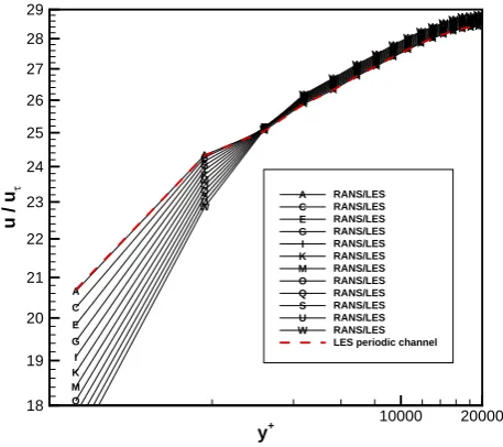
Fig. 4.Comparison of the mean velocity profile for nested channel flow simulation without body-force. Red dashed line: reference re-sults from the periodic channel simulation; black lines: mean veloc-ity profile at different sections of the channel with the buffer region.

in a discrete form as:

b

′_i

=

∆

T KE

u

′ i

∆

t

=

T KE

RAN S

u

′ i

∆

t

(20)

where, at the first time step, the velocity fluctuations are

com-puted from the mean velocity profile as

435

u

′i

=

c

i

U

RAN Si

R

(21)

being

c

i

a coefficient and

R

a suitable zero mean

colored

noise

function. After the first time step, the body-force gives

rise to velocity fluctuations in the buffer sub-domain, the

shear production term starts to extract energy from the mean

440

flow and the forcing term must adapt itself to the flow

condi-tions. This is accomplished by the proper definition in

Equa-tion 20 of the velocity scale, which is based on the actual

fluctuation level in the flow: an increased value of

u

′

i

corre-sponds to a decreased value of

b

′_i

and vice-versa. The velocity

445

fluctuations can be easily computed because the mean flow is

known at the boundary.

In order to provide a smooth transition from the buffer

sub-domain to the reference one, the forcing term is exponentially

damped to a target value

b

T

, which is zero, at the end of

450

the buffer region, subtracting to the function

b

i

(

x

)

the term

e

f(x)

(

b

i

(

x

)

−

b

T

(

x

))

.

Validation tests have been performed for the turbulent

plane-channel flow case, at

Re

τ

=

u

τ

δ/ν

= 20000

(with

u

τ

=

p

τ

w

/ρ

the friction velocity,

τ

w

the wall shear stress,

455

and

δ

the half height of the channel). It corresponds to a bulk

Reynolds number of the order of

10

6

, (Pope, 2000, pp.279) ,

Fig. 4. Comparison of the mean velocity profile for nested

chan-nel flow simulation without body force. Red dashed line: reference result from the periodic channel simulation; black lines: mean ve-locity profiles at different sections of the channel with the buffer region.

where, at the first time step, the velocity fluctuations are com-puted from the mean velocity profile as

u0_i=ciURANSiR, (21)

ci being a coefficient and R a suitable zero mean colored noise function. After the first time step, the body force gives rise to velocity fluctuations in the buffer sub-domain, the shear production term starts to extract energy from the mean flow and the forcing term must adapt itself to the flow con-ditions. This is accomplished by the proper definition in Eq. (20) of the velocity scale, which is based on the actual fluctuation level in the flow: an increased value of u0_i cor-responds to a decreased value ofb0_i and vice-versa. The ve-locity fluctuations can be easily computed because the mean flow is known at the boundary.

In order to provide a smooth transition from the buffer sub-domain to the reference one, the forcing term is expo-nentially damped to a target valuebT, which is zero, at the end of the buffer region, subtracting to the functionbi(x)the termef (x)(bi(x)−bT(x)).

Validation tests have been performed for the turbulent plane-channel flow case, at Reτ=uτδ/ν=20000 (with

uτ = √

τw/ρ the friction velocity,τw the wall shear stress, and δ the half height of the channel). It corresponds to a bulk Reynolds number of the order of 106 (Pope, 2000, p. 279), typical of environmental flows. Such a configura-tion is well suited for testing the nesting methodology, since there is no external instability source present in the channel except for the turbulence generated in the buffer sub-domain (see Keating et al., 2004 for a discussion).

(7)

A. Petronio et al.: LES model for wind-driven sea circulation in coastal areas 1101

A. Petronio et al.: LES model for wind driven sea circulation in coastal areas

7

I I I I I I I I I I I I

I I II

K K K K K K K KK KK K

K KKK

M M M M M M M MM MM M

MMMM O O O O O O O OO OO O

OOOO Q Q Q Q Q Q Q QQ QQ Q

QQQQ S S S S S S S SS SS S

S S SS

U U U U U U U UU UU U

U UUU

W W W W W W W WW WWW WWWW y+ u / uτ 10000 20000 18 19 20 21 22 23 24 25 26 27 28 29 RANS/LES RANS/LES RANS/LES RANS/LES RANS/LES RANS/LES RANS/LES RANS/LES LES periodic channel I K M O Q S U W

Fig. 5.Comparison of the mean velocity profile for nested channel flow simulation with body-force. Red dashed line: reference results from the periodic channel simulation; black lines: mean velocity profile at different sections of the channel with the buffer region.

I I I I I I I I I I I _I I I I I K K K K K K K K K K K K K K K _K M M M M M M M M M M M M M M M M O O O O O O O O O O O O O O O O Q Q Q Q Q Q Q Q Q Q Q _Q Q Q Q Q S S S S S S S S S S S S S S S _S U U U U U U U U U U U U U U U U W W W W W W W W W W W _W W W W W y/δ urm s

0 0.2 0.4 0.6 0.8 1

0 1 2 3 4 RANS/LES RANS/LES RANS/LES RANS/LES RANS/LES RANS/LES RANS/LES RANS/LES LES periodic channel I K M O Q S U W

Fig. 6.Comparison of the streamwise rms profile. Red dashed line: reference results from the periodic channel simulation; black lines: stream-wise rms profile at different sections of the channel with the buffer region.

typical of environmental flows. Such a configuration is well

suited to test the nesting methodology, since there is no

ex-ternal instability source present in the channel except for the

460

turbulence generated in the buffer sub-domain (see Keating

et al. (2004) for a discussion).

I I I I I I I I I I I I I

I I I K

K

K K _K K

K _K K _K

K K K

K K K M

M

M M M M M

M M _M M M M M _M M O O

O O _O O _O

O

O O O O O O _O

O Q

Q

Q Q Q Q _Q Q Q _Q Q _Q Q _Q Q Q S S

S S S S _S S _S

S S

S S _S S S U

U

U U U U U U _U U _U

U U _U U U W

W

W W W W W _W W

W W _W

W W _W W

y/δ vrm

s

0 0.2 0.4 0.6 0.8 1

0 1 2

3 RANS/LESRANS/LES

RANS/LES RANS/LES RANS/LES RANS/LES RANS/LES RANS/LES LES periodic channel I K M O Q S U W

Fig. 7.Comparison of the wall normal rms profile. Red dashed line: reference results from the periodic channel simulation; black lines: wall-normal rms profile at different sections of the channel with the buffer region.

I

I I _I I _I I I _I I I _I I I I I K _K K K K _K K K K K K K K _K K _K M M M M

M M _M M M M M _M M M M M O O _O O _O O O O O _O O _O O O O _O Q Q _Q

Q _Q Q

Q Q

Q

Q Q _Q Q _Q Q Q S S S S S S S _S S S S S _S S S S U U

U U U U _U U U U U U U U U _U W W W

W W W W W W W W W _W W _W W y/δ wrm s

0 0.2 0.4 0.6 0.8 1

0 1 2 3 RANS/LES RANS/LES RANS/LES RANS/LES RANS/LES RANS/LES RANS/LES RANS/LES LES periodic channel I K M O Q S U W

Fig. 8.Comparison of the spanwise rms profile. Red dashed line: reference results from the periodic channel simulation; black lines: span-wise rms profile at different sections of the channel with the buffer region.

A schematic representation of the case study is given in

fig. 3. The RANS inflow is applied at the left side of the

buffer sub-domain, colored in gray, in which turbulent

fluc-465

tuations are triggered. The indexes refer to different

cross-sections in which time averaged velocity profiles are

mon-Fig. 5. Comparison of the mean velocity profile for nested channel

flow simulation with body force. Red dashed line: reference result from the periodic channel simulation; black lines: mean velocity profiles at different sections of the channel with the buffer region.

A. Petronio et al.: LES model for wind driven sea circulation in coastal areas

7

I I I I I I I I I

I I I

I I II

K K K K K K K KK

KK K

K KKK

M M M M M M M MM

MM M

MMMM O O O O O O O OO

OO O

OOOO Q Q Q Q Q Q Q QQ

QQ Q

QQQQ S S S S S S S S S

SS S

S S SS

U U U U U U U UU

UU U

U UUU

I I I I I I I I I I I _I I I I _I K K K K K K K K K K K K K K K _K M M M M M M M M M M M M M M M M O O O O O O O O O O O _O O O O O Q Q Q Q Q Q Q Q Q Q Q Q Q Q Q Q S S S S S S S S S S S S S S S _S U U U U U U U U U U U _U U U U _U W W W W W W W W W W W _W W W _W W y/δ urm s

0 0.2 0.4 0.6 0.8 1

typical of environmental flows. Such a configuration is well

460

I I

I I _I

I I _I I _I I _I I _I I I K K

K K K

K

K _K

K

K K _K

K K

M M

M M M

M _M

M M _M _M

M M _M

M M

O O

O O _O

O _O

O O O O _O

O O

Q Q

Q Q Q Q _Q

Q _Q

Q Q _Q

Q _Q

Q Q

S S

S S S S _S

S _S

S S _S

S _S

S S

U U

U U U U U _U

U

U _U

U U _U

U U

W W

W W W _W _W

W _W

W W W

y/δ vrm

s

0 0.2 0.4 0.6 0.8 1

0 1 2

3 RANS/LESRANS/LES

RANS/LES RANS/LES RANS/LES RANS/LES RANS/LES RANS/LES LES periodic channel I K M O Q S U W

I

I I _I

I _I I I _I I I _I I I _I I K _K K _K K _K K K K K K K _K K K _K

M M _M

M

M M _M

M _M M M _M M M M M O _O

O O _O _O

O O O _O O _O O O O _O

Q Q _Q

Q _Q

Q Q

Q Q _Q

Q _Q

S S

S S _S

S _S S S S _S S S _S

U U _U

U U

U _U _U

U U U U _U U U _U

W W W _W _W

W _W W W W W _W W W _W W y/δ wrm s

0 0.2 0.4 0.6 0.8 1

Fig. 8.Comparison of the spanwise rms profile. Red dashed line: reference results from the periodic channel simulation; black lines: span-wise rms profile at different sections of the channel with the buffer region.

A schematic representation of the case study is given in

fluc-465

mon-Fig. 6. Comparison of the streamwise rms profile. Red dashed line:

reference result from the periodic channel simulation; black lines: streamwise rms profiles at different sections of the channel with the buffer region.

A schematic representation of the case study is given in Fig. 3. The RANS inflow is applied at the left side of the buffer sub-domain, colored in gray, in which turbulent fluc-tuations are triggered. The indexes refer to different cross-sections in which time-averaged velocity profiles are moni-tored along with second-order turbulence statistics. In the ex-ample depicted in Fig. 3, the buffer sub-domain spans from section 1 (A) to section 16 (H), whereas the reference sub-domain begins at section 17 (I).

A. Petronio et al.: LES model for wind driven sea circulation in coastal areas

7

I I I I I I I I I

I I I

I I II

K K K K K K K KK

KK K

K KKK

M M M M M M M MM

MM M

OO O

QQ Q

QQQQ S S S S S S S S S

SS S

S S SS

U U U U U U U UU

UU U

U UUU

I I I I I I I I I I I _I I I I _I K K K K K K K K K K K K K K K _K M M M M M M M M M M _M M M M M _M O O O O O O O O O O O O _O O O O Q Q Q Q Q Q Q Q Q Q Q _Q Q Q Q Q S S S S S S S S _S S S S S S S _S U U U U U U U U U U U _U U U U _U W W W W W W W W W W W W W W W W y/δ urm s

0 0.2 0.4 0.6 0.8 1

typical of environmental flows. Such a configuration is well

460

I I

I I _I

I I _I I _I I _I I _I I I K K

K K _K

K K _K K _K K _K K _K K K M M

M M M

M _M

M M _M

M _M

M M

O O

O O _O

O O O O O _O

O O

Q Q

Q Q Q Q _Q

Q _Q

Q Q _Q

Q _Q

Q Q

S S

S S S S S _S

S

S S _S

S _S

S S

U U

U U U U U U _U

U _U

U U _U

U U

W W

W W W W W _W

W _W W _W W _W W W y/δ vrm s

0 0.2 0.4 0.6 0.8 1

I

I I _I

I _I I I _I I I _I I I _I I K _K K _K K _K K K _K K K _K K _K K _K

M M M _M

M M _M

M M M M _M M _M M M O _O

O O _O _O

O O O _O O _O O O O _O Q _Q

Q Q _Q

Q _Q

Q Q _Q

Q _Q

S S

S S _S

S _S S S S _S S S _S

U U _U

U U U U U _U U _U U _U

W W W _W _W

W _W

W

W _W

W

W W _W

y/δ wrm

s

0 0.2 0.4 0.6 0.8 1

Fig. 8. Comparison of the spanwise rms profile. Red dashed line: reference results from the periodic channel simulation; black lines: span-wise rms profile at different sections of the channel with the buffer region.

A schematic representation of the case study is given in

fluc-465

mon-Fig. 7. Comparison of the wall-normal rms profile. Red dashed line:

reference result from the periodic channel simulation; black lines: wall-normal rms profiles at different sections of the channel with the buffer region.

A. Petronio et al.: LES model for wind driven sea circulation in coastal areas

7

I I I I I I I I I I

I I I I II

K K K K K K K KK

KK K

K KKK

M M M M M M M MM

MM M

OO O

QQ Q

QQQQ S S S S S S S SS

SS S

S S SS

U U U U U U U UU

UU U

U UUU

W W W W W W WW WW WWWWWW y+ u / uτ 10000 20000 18 19 20 21 22 23 24 25 26 27 28 29 RANS/LES RANS/LES RANS/LES RANS/LES RANS/LES RANS/LES RANS/LES RANS/LES LES periodic channel I K M O Q S U W

I I I I I I I I I I I _I I I I _I K K K K K K K K K K K K K K K _K M M M M M M M M M M M M M M M M O O O O O O O O O O O _O O O _O O Q Q Q Q Q Q Q Q Q Q Q _Q Q Q Q Q S S S S S S S S _S S S S _S S S S U U U U U U U U U U _U U U U U U W W W W W W W W W W W W W W _W W y/δ urm s

0 0.2 0.4 0.6 0.8 1

typical of environmental flows. Such a configuration is well

460

I I

I I _I

I

I _I

I

I I _I

I I

K K

K K _K

K _K

K _K<