Inﬂuence of dynamic vegetation on climate change and terrestrial carbon storage in the Last Glacial Maximum

(1)

Clim. Past, 9, 1571–1587, 2013 www.clim-past.net/9/1571/2013/ doi:10.5194/cp-9-1571-2013

EGU Journal Logos (RGB)

Advances in

Geosciences

Open Access

Natural Hazards

and Earth System

Sciences

Open Access

Annales

Geophysicae

Open Access

Nonlinear Processes

in Geophysics

Open Access

Atmospheric

Chemistry

and Physics

Open Access

Atmospheric

Chemistry

and Physics

Open Access Discussions

Atmospheric

Measurement

Techniques

Open Access

Atmospheric

Measurement

Techniques

Biogeosciences

Open Access Open Access

Biogeosciences

Discussions

Climate

of the Past

Climate

of the Past

Discussions

Earth System

Dynamics

Earth System

Dynamics

Discussions

Geoscientific

Instrumentation

Methods and

Data Systems

Open Access

Geoscientific

Instrumentation

Methods and

Data Systems

Geoscientific

Model Development

Geoscientific

Model Development

Discussions

Hydrology and

Earth System

Sciences

Open Access

Hydrology and

Earth System

Sciences

Ocean Science

Discussions

Solid Earth

Discussions

The Cryosphere

Discussions

Natural Hazards

and Earth System

Sciences

Open Access

Discussions

Influence of dynamic vegetation on climate change and terrestrial

carbon storage in the Last Glacial Maximum

R. O’ishi1,2and A. Abe-Ouchi1,3

1_{Atmosphere and Ocean Research Institute, University of Tokyo, Kashiwa, Japan} 2_{National Institute of Polar Research, Tokyo, Japan}

3_{Frontier Research Center for Global Change, Yokohama, Japan} Correspondence to: R. O’ishi ([email protected])

Received: 5 November 2012 – Published in Clim. Past Discuss.: 27 November 2012 Revised: 10 May 2013 – Accepted: 3 June 2013 – Published: 22 July 2013

Abstract. When the climate is reconstructed from

paleoev-idence, it shows that the Last Glacial Maximum (LGM, ca. 21 000 yr ago) is cold and dry compared to the present-day. Reconstruction also shows that compared to today, the vege-tation of the LGM is less active and the distribution of veg-etation was drastically different, due to cold temperature, dryness, and a lower level of atmospheric CO2

concentra-tion (185 ppm compared to a preindustrial level of 285 ppm). In the present paper, we investigate the influence of vege-tation change on the climate of the LGM by using a cou-pled atmosphere-ocean-vegetation general circulation model (AOVGCM, the MIROC-LPJ). The MIROC-LPJ is different from earlier studies in the introduction of a bias correction method in individual running GCM experiments. We exam-ined four GCM experiments (LGM and preindustrial, with and without vegetation feedback) and quantified the strength of the vegetation feedback during the LGM. The result shows that global-averaged cooling during the LGM is amplified by +13.5 % due to the introduction of vegetation feedback. This is mainly caused by the increase of land surface albedo due to the expansion of tundra in northern high latitudes and the desertification in northern middle latitudes around 30◦N to 60◦N. We also investigated how this change in cli-mate affected the total terrestrial carbon storage by using of-fline Lund-Potsdam-Jena dynamic global vegetation model (LPJ-DGVM). Our result shows that the total terrestrial car-bon storage was reduced by 597 PgC during the LGM, which corresponds to the emission of 282 ppm atmospheric CO2. In

the LGM experiments, the global carbon distribution is gen-erally the same whether the vegetation feedback to the at-mosphere is included or not. However, the inclusion of

veg-etation feedback causes substantial terrestrial carbon storage change, especially in explaining the lowering of atmospheric CO2during the LGM.

1 Introduction

Paleoenvironmental reconstructions indicate a cold period around 21 000 yr ago, known as the Last Glacial Maximum (LGM), which is characterized by the huge extension of an ice sheet and lower atmospheric CO2concentration.

Recon-struction indicates that two huge ice sheets covered the north-ern part of the North American continent and northnorth-ern Eu-rope (Peltier, 1994, 2004). An equivalent amount of sea wa-ter is removed from the LGM ocean, so that sea level during the LGM is lower by 120 to 150 m than that of the present-day (Yokoyama et al., 2000). Paleo-ocean reconstruction shows about 2 to 3◦C cooling of the sea-surface tempera-ture compared to the present-day in the tropical ocean and more than 10◦C cooling in high latitudes (CLIMAP Project Members, 1976, 1984; Kucera et al., 2005; Waelbroeck et al., 2009). Pollen-based reconstruction also indicates more than 10◦_{C cooling of ice-free land in North America and Europe}

(Bartlein et al., 2011). A cooler climate reduces precipitation, thus the land surface is drier than at present-day (Kohfeld and Harrison, 2000; Yu et al., 2000). Reconstructed infor-mation from ice-core components indicates that the atmo-spheric CO2concentration during the LGM is about 185 ppm

(2)

1572 R. O’ishi and A. Abe-Ouchi: Climate and vegetation/carbon change in the LGM

distribution during the LGM is different from that of today in that it included an expanded arid area, a southward shift of the boreal forest belt, and a southward expansion of tundra (Prentice and Webb, 1998; Prentice and Jolly, 2000; Prentice and Harrison, 2009).

The paleoclimate modeling community tried to reproduce the LGM climate by using atmosphere general circulation models (AGCMs) and coupled atmosphere-ocean general circulation models (AOGCMs) in the Paleoclimate Model-ing Intercomparison Project (PMIP). The results of the PMIP show that general circulation models (GCMs) are generally able to reproduce consistent cooling (Joussaume and Taylor, 2000; Braconnot et al., 2007). The paleovegetation distribu-tion during the LGM is also investigated, using vegetadistribu-tion models with GCM results as input. This predicted qualita-tively consistent vegetation changes with climate change in the LGM (Harrison and Prentice, 2003; Prentice et al., 2011). To introduce vegetation-climate feedback into GCMs, cou-pled atmosphere-ocean-vegetation GCMs (AOVGCMs) are developed. By using the AOVGCMs for the LGM experi-ments, these models well reproduce both climate and veg-etation change in the LGM compared to the present-day (Wyputta and McAvaney, 2001; Ganopolski, 2003; Crucifix et al., 2005a; Crucifix et al., 2005b; Crucifix and Hewitt, 2005; Jahn et al., 2005; Henrot et al., 2009). These results reveal how changes in the land surface during the LGM contributes to the climate through changes of surface heat and water balance. Dust emission change due to vegetation change is also noted as an important factor of the vegetation during the LGM (Mahowald et al., 2006; Takemura et al., 2009).

Another aspect of vegetation change during the LGM is the change in the carbon cycle that affects atmospheric CO2

concentration. Not only the distribution of vegetation but also the strength of photosynthesis and soil carbon decomposi-tion are important factors in terrestrial carbon distribudecomposi-tion (Gerber et al., 2004; Prentice and Harrison, 2009). As far as the terrestrial carbon storage, reconstruction indicates a 300 to 700 PgC reduction during the LGM (Bird et al., 1994), and estimation by LGM simulation with GCMs shows al-most the same range of terrestrial carbon reduction (Prentice et al., 1993; Friedlingstein et al., 1995; François et al., 1998, 1999; Kaplan et al., 2002; Otto et al., 2002; Köhler and Fischer, 2004; Köhler et al., 2005; Ciais et al., 2011). For this kind of prediction of past terrestrial carbon storage in-cluding LGM, it is usual to use a dynamic global vegetation model (Joos et al., 2004).The uncertainty around the amount of terrestrial carbon stored during the LGM is thus larger than 200 PgC, which is equivalent to a reduction in the atmo-sphere of 100 ppm CO2(Jouzel et al., 1993; Monnin et al.,

2001). If we consider the sea level change during the LGM, about 200 PgC could have been stored in the exposed con-tinental shelf (Faure et al., 1996; Zeng, 2003; Montenegro et al., 2006), and the uncertainty in this may be comparable to that of the change in atmospheric CO2.

As shown above, there is uncertainty in the amount of change in terrestrial carbon, but it is important for under-standing the LGM environment, especially the change in atmospheric CO2. In the present study, we newly apply a

bias correction procedure in a running AOVGCM to reduce unrealistic vegetation feedback caused by temperature and precipitation bias. Then we investigate the climate of the LGM, the vegetation feedback onto the climate and the resul-tant equilibrium carbon storage with this newly constructed bias-corrected AOVGCM in order to quantify vegetation-atmosphere feedback in the LGM and also quantify which aspect of the LGM influences the terrestrial carbon storage in the LGM. To save integration time, we actually use a slab-ocean instead of a full slab-ocean general circulation model as a component of our AOVGCM. We also run several offline vegetation model experiments to obtain the equilibrium car-bon storage which corresponds to climate of these AOVGCM experiments as input to an offline experiment. In the present study, we separate difference of terrestrial carbon storage into three kinds: response to the LGM climate, washout by ice-sheet coverage, and the new stock on the exposed continen-tal shelf. We also apply the AOGCM for the LGM in order to evaluate the vegetation-climate feedback during the LGM and to use the equilibrium climate as input to the vegetation module, and also to estimate how vegetation evaluation after the AOGCM differs from the result that was consistent with those of the AOVGCM.

2 Model description

2.1 Model components

In the present study, a coupled vegetation general circu-lation model MIROC-LPJ (O’ishi and Abe-Ouchi, 2011) is used. The atmosphere component of the MIROC-LPJ is CCSR/NIES/FRCGC AGCM (Center for Climate Sys-tem Research/National Institute for Environmental Stud-ies/Frontier Research Center for Global Change atmospheric general circulation model), which is the same as the atmo-spheric part of an atmosphere-ocean coupled GCM known as the Model for Interdisciplinary Research on Climate (MIROC) (Hasumi and Emori, 2004) that contributed to the fourth assessment report of the Intergovernmental Panel on Climate Change (IPCC AR4)(Meehl et al., 2007).

(3)

R. O’ishi and A. Abe-Ouchi: Climate and vegetation/carbon change in the LGM 1573

by the atmosphere component are used as the input to the LPJ-DGVM. The terrestrial heat and energy component of MIROC is Minimal Advanced Treatments of Surface Inter-action and RunOff (MATSIRO; Takata et al., 2003), which does not include a dynamical vegetation component. In this version of MIROC, fractional coverage of different vegeta-tion types is not yet included and just one vegetavegeta-tion type represents one land grid cell. Hence we coupled MIROC and LPJ-DGVM in a very simple way. LPJ-DGVM only predicts representative vegetation type (which is classified in MAT-SIRO) for every grid cell annually. Since LPJ-DGVM is able to predict the distribution of ten PFT types, we translate this combination of PFTs into MATSIRO vegetation classifica-tion with some addiclassifica-tional informaclassifica-tion (leaf area index (LAI), soil moisture, growing degree days (GDD), net primary pro-ductivity (NPP); see O’ishi and Abe-Ouchi, 2009, for detail). This translated vegetation distribution does not include ex-act information from LPJ-DGVM but substantial large-scale characteristics of vegetation distribution. Since LPJ-DGVM does not handle human-induced change (e.g crops), all “veg-etation” in the present study is inevitably potential vegeta-tion. Then MATSIRO solves land surface heat and energy budget and balance equations according to the vegetation type (translated from LPJ-DGVM) and corresponding pa-rameters which are based on MATSIRO vegetation classifi-cation. We simplified LAI seasonality as a simple sine curve which is also based on MATSIRO vegetation classification. Thus in MIROC-LPJ, MATSIRO is able to work if a vegeta-tion type is given in a grid cell whether it is from LPJ-DGVM or not. We can also choose a specific prescribed vegetation distribution instead of coupling LPJ-DGVM (this kind of ex-periment is noted as fixed vegetation in Sect. 3.1).

The original MIROC includes a full ocean dynamical component COCO (Hasumi, 2006), but it will take too long a numerical integration to equilibrate because atmosphere-ocean-vegetation interactive system may have several hun-dred years (perhaps 1000 yr or more) of time scale to achieve the equilibrium. In the present study, we actually choose a slab-ocean model for an ocean component of MIROC-LPJ instead of the COCO to save integration time. We assume seasonality of ocean heat transport to predict distribution of sea surface temperature and sea-ice.

In all experiments, the horizontal and vertical resolu-tions of the atmospheric correspond to T42 (2.8×2.8◦ longitude×latitude) and 20 layers, respectively. Horizontal resolution of slab-ocean component is also T42.

2.2 Bias correction

The MIROC generally reproduces the climate of today and the 20th century, but there is an unavoidable temperature and precipitation bias in the MIROC compared to the observa-tions as a benchmark (The European Centre for Medium-Range Weather Forecasts (ECMWF) ERA40 temperature (Uppala et al., 2005) and the CPC Merged Analysis of

Pre-cipitation (Xie and Arkin, 1997)). This bias can cause an incorrect distribution of vegetation in the preindustrial and present-day, and thus can cause a unrealistic response of the atmosphere to the change of vegetation distribution in the paleo-setting experiments. Hence we introduce a bias cor-rection into the MIROC-LPJ. The monthly temperature and precipitation from the AGCM are modified by using a refer-ence model experiment and observed data, in order to remove the bias before these variables are passed to the LPJ-DGVM as follows:

Tinput=Tmodel−(TPD,model−Tobs) (1)

Pinput=Pmodel·

Pobs

PPD,model

(2)

whereTmodelandPmodelare surface air temperature and

pre-cipitation predicted in an MIROC-LPJ experiment.Tobsand Pobs are present-day observational surface air temperature

and precipitation which correspond to ECMWF ERA40 and CMAP, respectively).TPD,modelandPPD,modelare surface air

temperature and precipitation, respectively, predicted in the present-day MIROC-LPJ experiment which adopts an atmo-spheric CO2concentration of 345 ppm without this bias

(4)

1574 R. O’ishi and A. Abe-Ouchi: Climate and vegetation/carbon change in the LGM

gap (covered with grass) appears between boreal and temper-ate in the control preindustrial experiment if we do not apply bias correction (Fig. A1a). This unrealistic gap will expand northward if we try to carry out various kinds of warming simulations and cause more discrepancy between the control and warming experiments. When we try to run the LGM sim-ulation (Fig. A1b), there is a northward shift of boreal forest in Siberia in spite of the cool climate. This strange result is considered to be induced by the combined effect of a warm bias, decrease of snow cover and a warming due to the sta-tionary wave effect of the Scandinavian ice sheet (Abe-Ouchi et al., 2007).

2.3 Carbon balance

The LPJ-DGVM (Sitch et al., 2003) is able to predict four types of biomass storage (leaf, heartwood, sapwood, and root) for every PFT, carbon pools that correspond to different time scales of decomposition, in the coupled MIROC-LPJ. At first, the net primary productivity (NPP) is calculated by the gross primary productivity, autotrophic respiration and growth cost of production. Then NPP is distributed to four biomass carbon pools shown above. Biomass is moved to soil carbon pool by turnover, fire event, heat stress and change of bioclimatic limits. The soil carbon is separated into three pools with different time scale of decomposition. The decomposition of soil carbon depends on temperature, soil moisture and time scale of decomposition. LPJ-DGVM employs the relation between temperature and soil carbon decomposition from Lloyd and Taylor (1994).

Different from full carbon coupled GCM experiments (e.g. Faloon et al., 2012), feedback through carbon balance is not introduced in the MIROC-LPJ and both the GCM and LPJ-DGVM are forced by a given level of atmospheric CO2. This is because we intend to evaluate the direct

ef-fect of vegetation change as land surface boundary condi-tion through water and heat balance upon the climate. Pre-diction of the equilibrium terrestrial carbon is completed by an offline LPJ-DGVM experiment using as input the result of the MIROC-LPJ equilibrium climate. These offline ex-periments are conducted because it takes many integration years to equilibrate the terrestrial carbon storage in a cou-pled MIROC-LPJ setup (see Experimental settings, below). Another reason is the limitation of MIROC itself because this version of MIROC (and therefore MIROC-LPJ) does not include ocean carbon cycle.

3 Experimental settings

3.1 Coupled GCM experiments

Two experiments are preformed by using the MIROC-LPJ, as shown in Table 1. In the preindustrial control experi-ment, AOV(PI), the preindustrial level of atmospheric CO2

(285 ppm) and present-day orbital parameters are employed.

In the LGM experiment, AOV(LGM), the LGM level of at-mospheric CO2(185 ppm), the LGM orbital parameters, and

ICE-5G ice sheets (Peltier, 2004) are taken from the Paleo-climate Modeling Intercomparison Project 2 (PMIP2) proto-col (Braconnot et al., 2007). The expanded LGM land cover (+23×1012m2) is employed by assuming a 150 m sea level descent which is the largest estimation (Yokoyama et al., 2000) in order to evaluate the upper limit of the effect of difference of coastline, especially for vegetation distribution and carbon storage. Other green house gases (GHGs), CH4,

N2O, CFC and O3are set to the preindustrial values because

we intend to extract response of climate and vegetation to difference of atmospheric CO2. These experiments are

in-tegrated over about 400 yr including spin-up, which is long enough to reach equilibrium for both vegetation distribution and climate.

An additional set of experiments, AO(PI) and AO(LGM), are performed to investigate the effect of vegetation change on climate. In these experiments, the model does not refer the LPJ-DGVM, and the vegetation map is fixed to the equi-librium state of the AOV(PI) experiment. For this, we first extract MATSIRO vegetation type which appeared most fre-quently during the last 50 yr of AOV(PI) in each grid cells. This vegetation map is considered to be a representative veg-etation distribution which is given to MATSIRO as a surface boundary condition during the last 50 yr of AOV(PI). Then we run MIROC-LPJ with this vegetation map instead of LPJ-DGVM’s prediction. As noted in Sect. 2.1, MIROC-LPJ is able to run without vegetation index from LPJ-DGVM since vegetation type is used to choose a set of parameters which is defined for every vegetation type. In AO(LGM), we use the same coastline and ice-sheet distribution as AOV(LGM). Thus, in order to prepare a vegetation map in the AO(LGM), an offline LPJ-DGVM experiment is performed using the LGM coastline with the AOV(PI) result as input. This map is the same as the resultant vegetation map of the AOV(PI) for those land grid cells that are shared by both the preindus-trial and the LGM. Results of the last 50 yr in all experiments are used for the analysis since vegetation distribution and cli-mate are sufficiently equilibrated with 400 yr integration in both AOV(PI) and AOV(LGM).

3.2 Offline LPJ-DGVM experiments

3.2.1 Sensitivity experiments

We perform six sensitivity experiments, as shown in Table 2, using the LPJ-DGVM in an offline mode. In order to compare the impact of CO2concentration, precipitation, and

temper-ature on vegetation distribution during the LGM (which is similar method to Jones et al., 2004; Faloon et al., 2011), one or two factor(s) are set to the LGM value and the rest to the preindustrial for input to the LPJ-DGVM. Atmospheric CO2

(5)

Table 1. Settings of the experiments performed in this study.

Experiment CO2level Orbit Vegetation MIROC-LPJ offline LPJ-DGVM

AOV(PI) 285 ppm 0ka dynamic 390 yr 1000 yr AOV(LGM) 185 ppm LGM dynamic 400 yr 1000 yr AO(PI) 285 ppm 0ka fixed to AOV(PI) 75 yr – AO(LGM) 185 ppm LGM fixed to AOV(PI) 50 yr 1000 yr

Table 2. Settings of the offline sensitivity experiments performed

in this study. Precipitation and temperature are taken from the AOV(LGM) and the AOV(PI), respectively.

Experiment CO2 Precipitation Temperature integration

CP 185 ppm LGM PI 1000 yr

TC 185 ppm PI LGM 1000 yr

TP 285 ppm LGM LGM 1000 yr

T 285 ppm PI LGM 1000 yr

P 285 ppm LGM PI 1000 yr

C 185 ppm PI PI 1000 yr

Temperature and precipitation are taken from the last 50 yr time series of both AOV(LGM) and AOV(PI) to include the interannual variability, and used 20 times repeatedly for 1000 yr of integration; the results of the last 100 yr are used for analysis.

3.2.2 Carbon equilibrium

Since changes in soil carbon have a long time scale, approx-imately four hundred years of AOVGCM integration in Ta-ble 1 is too short to equilibrate the total terrestrial carbon stor-age. In analogy to the experiments described in Sect. 3.2.1 (Table 2), we performed further 1000 yr-long offline experi-ments but now using the full forcings derived from our two AOVGCM experiments. In order to evaluate the equilibrium carbon storage in the LGM and the preindustrial era, offline LPJ-DGVM experiments are performed, using the result of the last 50 yr time series in the two AOVGCM experiments as input and letting them run for the equivalent of 1000 yr by giving climate variables 20 times repeatedly. The vegetation map and the climate are equilibrated far faster than terres-trial carbon storage, so that it is not necessary to integrate a coupled MIROC-LPJ until carbon storage is equilibrated. This is the same procedure as was adopted in a previous study (O’ishi and Abe-Ouchi, 2009). We also examine offline LPJ-DGVM experiments, using the result of the AO(LGM) experiment as input. This experiment corresponds to the of-fline diagnosis of carbon storage using a GCM result without vegetation feedback as well as Harrison and Prentice (2003). The last 100 yr of resultant variables are used for analysis. Carbon storages/fluxes are just averaged over the last 100 yr. Hence vegetation distribution is predicted by vegetation in-dices with interannual variability, we choose and show the

most dominant vegetation index during the last 100 yr as a representative vegetation index.

4 Results

4.1 Vegetation distribution

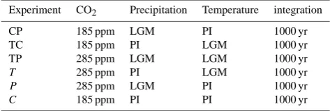
In the AOV(LGM), there are some typical changes in the veg-etation pattern compared to the AOV(PI) (Fig. 1a and b). We first discuss changes in vegetation as determined according to the MATSIRO classification. In the south of the Scandi-navian and Laurentide ice sheets, boreal forests shift south-ward and tundra appears. In eastern Siberia, boreal forests retreat southward and the southern boundary of tundra is re-located to 50 N. The southern boundary of the boreal forests also shifts southward in North America and China. In the downstream region of the Scandinavian ice sheet, a slight northward shift of boreal forest appears. Total reduction of the area of boreal forest is 14.0×1012m2and expansion of tundra is 6.2×1012m2. Expansion of desert is seen in Central Asia, North and South Africa, and North America, totaling 15.1×1012m2of increase. In the tropical region, the tropical forest shrinks, and savanna or grassland appears or increases, especially in Africa. Tropical forest covers the exposed con-tinental shelf over the maritime continent. The concon-tinental shelf of the East China Sea to south of the Japan Sea is cov-ered by temperate forest. The East Siberian Sea and north of the Bering Sea turns into tundra. According to LPJ-DGVM PFT classification, a fraction of grass PFTs in LPJ-DGVM increase in high latitude (Fig. 1c) and decreases in the cen-tral Eurasia. A fraction of forest shows a decrease in both northern high latitudes and tropical regions (Fig. 1d). The NPP also shows a drastic change (Fig. 3a and h). The global total annual NPP during the LGM and the preindustrial are 44.0 PgC yr−1and 59.5 PgC yr−1, respectively (Table 3). Re-duction of 5.4 PgC yr−1 _{occurs due to covering by the}

ex-panded ice sheet, and an increase of 7.5 PgC yr−1_{occurs on}

the exposed continental shelf due to a change in sea level (these values are not shown in the table). In the AOV(LGM), a large part of the total reduction of NPP is seen in the forest region (see Fig. 3h) compared to AOV(PI).

(6)

1576 R. O’ishi and A. Abe-Ouchi: Climate and vegetation/carbon change in the LGM

Discussion

P

ap

er

|

Discussion

P

ap

er

|

Discussion

P

ap

er

|

Di

scuss

ion

P

ap

er

|

(a) Vegetation distribution in AOV(PI)

(b) Vegetation distribution in AOV(LGM)

(c) Difference of grass fraction [AOV(LGM) - AOV(PI)]

(d) Difference of forest fraction [AOV(LGM) - AOV(PI)]

-0.4 -0.2 -0.1 0.1 0.2 0.4

Tropical evergreen Tropical deciduous Boreal conifer

Savanna Grassland Desert

Tundra Ice Temperate mixed

Boreal deciduous

Fig. 1.

Vegetation distribution obtained in (a)

AOV(PI)

and (b)

AOV(LGM)

according to

MAT-SIRO classification.

Difference of fractional coverage in (c) grass and (d) forest between

AOV(LGM)

and

AOV(PI)

which are from PFT-based variables in the LPJ-DGVM.

36

Fig. 1. Vegetation distribution obtained in (a) AOV(PI) and (b) AOV(LGM) according to MATSIRO classification. Difference of fractional

coverage in (c) grass and (d) forest between AOV(LGM) and AOV(PI) which are from PFT-based variables in the LPJ-DGVM.

Table 3. Equilibrium global NPP (PgC yr−1) and global biomass, soil carbon and total carbon storage (PgC). The sum of four biomass carbon pools is shown as “biomass”. The sum of three soil carbon pools is shown as “soil carbon”. Total carbon is sum of biomass and soil carbon. Values in the parentheses do not include the LGM ice-sheet area in the preindustrial nor continental shelf area in the LGM to extract pure response to climate and atmospheric CO2. Result

of AOV(PI) and upper column of other experiments are absolute values. In lower columns, values denote absolute differences with respect to AOV(PI). The last digit can include a rounding error.

Experiment NPP Biomass Soil carbon Total

AOV(PI) 59.5 (54.0) 1082 (973) 1368 (1088) 2450 (1062) AOV(LGM) 44.0 (36.5) 828 (672) 1025 (888) 1853 (1560)

−15.5 (−17.6) −254 (−301) −343 (−200) −597 (−502) AO(LGM) 44.6 (36.7) 823 (660) 1009 (861) 1831 (1522)

−14.9 (−17.3) −259 (−313) −359 (−227) −619 (−540) CP 44.2 (36.7) 808 (653) 853 (765) 1661 (1417)

−15.3 (−17.4) −274 (−321) −515 (−323) −789 (−645) TC 48.5 (40.2) 933 (760) 1207 (1033) 2140 (1793)

−11.0 (−13.8) −149 (−213) −161 (−55) −310 (−269) TP 57.7 (47.9) 1068 (875) 1316 (1141) 2384 (2016)

−1.8 (−6.2) −14 (−98) −52 (+53) −66 (−46)

T 64.1 (53.2) 1218 (1001) 1503 (1298) 2721(2299) +4.6 (−0.8) +136 (+28) +135 (+210) +271 (+237)

P 59.7 (49.5) 1047 (856) 1101 (984) 2148 (1840) +0.2 (−4.5) −35 (−117) −267 (−104) −302 (−222)

C 49.3 (41.0) 929 (761) 961 (859) 1890 (1620)

−10.2 (−13.0) −153 (−212) −407 (−229) −560 (−442)

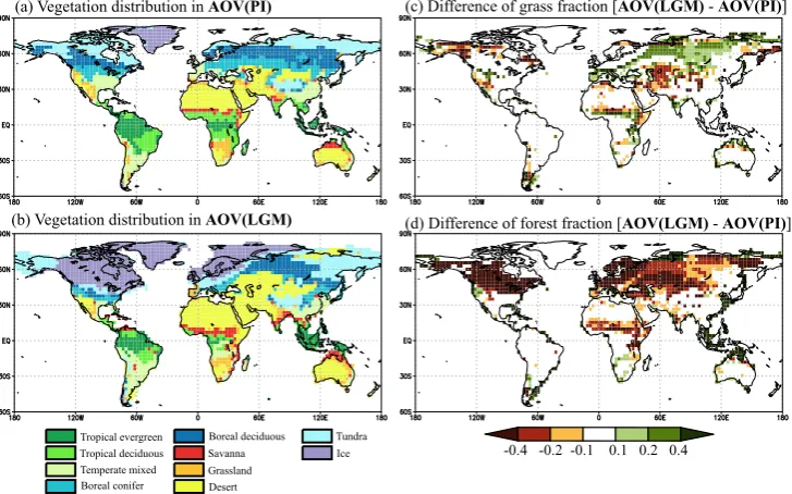
aspects of environmental change during the LGM. These re-sults are compared with AOV(PI) and AOV(LGM) in Fig. 2 according to the MATSIRO classification. Of course an of-fline experiment is conceptually different from an online ex-periment, however, the response signals to different temper-ature, precipitation and CO2concentration are far larger than

the inconsistency between offline and online. By comparing the left side of Fig. 2 (a–d, preindustrial temperature) and the right side of Fig. 2 (e–h, LGM temperature), it is shown that the temperature changes during the LGM mainly dom-inated the distribution of forest/tundra boundary. Cooling in high latitudes shifts the boundary of the forest/tundra to the south. Around the Scandinavian and Laurentide ice sheets, tundra appears between the ice sheet and the boreal forests, due to cooling, in all offline experiments with LGM temper-ature (Fig. 2e–h). In the tropical regions, cooling compen-sated for expansion of savanna, which is due to less pre-cipitation and lower CO2 during the LGM but a relatively

higher preindustrial temperature. For example, with LGM temperature (Fig. 2h), savanna is replaced by forest, com-pared to correspondent experiments with preindustrial tem-perature (Fig. 2d). This tendency is also seen in other com-binations of precipitation and CO2(e.g comparison between

Fig. 2a and e, between Fig. 2b and f and between Fig. 2c and g). This is consistent with NPP changes. In Fig. 3e, reduc-tion of NPP in tropical region is smaller due to decrease of autotrophic respiration if we apply LGM temperature.

(7)

R. O’ishi and A. Abe-Ouchi: Climate and vegetation/carbon change in the LGM 1577

Discussion

P

ap

er

|

Discussion

P

ap

er

|

Discussion

P

ap

er

|

Di

scuss

ion

P

ap

er

|

(a) AOV(PI)

(b) offline exp. P

(c) offline exp. C

(d) offline exp. CP

(e) offline exp. T

(f) offline exp. TP

(g) offline exp. TC

(h) AOV(LGM)

Fig. 2.

Vegetation distribution obtained in (a)

AOV(PI)

and (h)

AOV(LGM)

(they are as same as

Figure 1 and shown again for convenience). Vegetation distribution obtained in offline sensitivity

experiments (b)

P

, (c)

C

, (d)

CP

, (e)

T

, (f)

TP

and (g)

TC

according to MATSIRO classification.

37

Fig. 2. Vegetation distribution obtained in (a) AOV(PI) and (h) AOV(LGM) (they are as same as Fig. 1 and shown again for convenience).

Vegetation distribution obtained in offline sensitivity experiments (b)P, (c)C, (d) CP, (e)T, (f) TP and (g) TC according to MATSIRO classification.

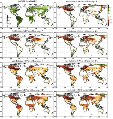
of desert and savanna. Especially the boundary between bo-real forests and desert is formed by LGM precipitation. In the central Eurasia continent, less precipitation during the LGM expands deserts, especially north and west of the Caspian Sea, which had the largest decrease in precipitation on the Eurasian continent. The Gobi and Taklamakan deserts ex-pands slightly northward. The boreal forests of the Pamir plateau and Tian Shan Mountains turns into desert, due to the decrease in precipitation. However, the total shift of this for-est/desert boundary is not achieved solely by LGM precipita-tion (Fig. 2b) but addiprecipita-tional combined effect with LGM CO2

(Fig. 2d) is also important. The expansion of desert and sa-vanna corresponds to change of NPP. Figure 3b indicates ma-jor reduction of NPP in central Eurasia and Sahel in Africa.

Other experiments with LGM precipitation (Fig. 3d, f and h) show the same pattern of NPP change in these regions.

By comparing Fig. 2c, d, g and h (with LGM CO2) and

Fig. 2a, b, e and f (with preindustrial CO2), we see that low

CO2during the LGM mainly dominated the distribution of

savanna in the tropical region e.g. Sahel, South Africa and Australia (Fig. 2c for example). There is a slight expansion of desert due to decrease photosynthesis, but the NPP shows a substantial reduction due to the lower level of CO2not only

in the tropical region but also in temperate and boreal forests (Fig. 3c).

(8)

1578 R. O’ishi and A. Abe-Ouchi: Climate and vegetation/carbon change in the LGM

Discussion

P

ap

er

|

Discussion

P

ap

er

|

Discussion

P

ap

er

|

Di

scuss

ion

P

ap

er

|

(a) NPP in AOV(PI)

(b) Relative NPP in offline exp. P

(c) Relative NPP in offline exp. C

(d) Relative NPP in offline exp. CP

(e) Relative NPP in offline exp. T

(f) Relative NPP in offline exp. TP

(g) Relative NPP in offline exp. TC

(h) Relative NPP in AOV(LGM)

Fig. 3.

Equilibrium Net Primary Productivity (NPP) [kg/m

2

/yr] in (a)

AOV(PI)

and absolute NPP

differences with respect to

AOV(PI)

in offline experiments (b)

P

, (c)

C

, (d)

CP

, (e)

T

, (f)

TP

and

(g)

TC

. Absolute NPP difference in

AOV(LGM)

with respect to

AOV(PI)

is shown in (h).

38

Fig. 3. Equilibrium net primary productivity (NPP) [kg m−2yr−1] in (a) AOV(PI) and absolute NPP differences with respect to AOV(PI) in offline experiments (b)P, (c)C, (d) CP, (e)T, (f) TP and (g) TC. Absolute NPP difference in AOV(LGM) with respect to AOV(PI) is shown in (h).

The other boundary between boreal forest and desert in mid-latitudes is most influenced by precipitation decrease. Low CO2levels also contribute to vegetation shift but the

magni-tude is smaller in mid-latimagni-tudes. In tropical areas, the lower atmospheric CO2 during the LGM only changes the

vege-tation into savanna, and it reduces the NPP, even when the vegetation distribution is unchanged. There are also synergy effects of the three different forcing factors. In Amazonia and Africa, temperate forest replaces tropical forest, so that the tropical regions shrink toward the equator. This is not only due to cooling but also to precipitation and CO2. The

south-ward shift of the tundra/forest boundary in northeast China is not explained by a single variable. A synergy effect of temperature, precipitation, and CO2causes the total response

of vegetation in these regions. However, a total amount of these synergy effects is limited. The response of NPP, which explains vegetation change well, indicates that temperature,

precipitation and CO2effects are almost additive (Table 3).

The sum of individual responses of NPP to temperature (T,

−0.8 PgC yr−1_{), precipitation (}_P_,₋_{4.5 PgC yr}−1_{) and CO} 2

(C,−13.0 PgC yr−1_{) is very close to that of total AOV(LGM)}

responses (−17.6 PgC yr−1). A synergy effect is seen be-tween temperature and precipitation by comparing TP result (−6.2 PgC yr−1) with the sum ofT andP. Synergy of pre-cipitation and CO2(CP,−17.4 PgC yr−1) shows close value

to that of AOV(LGM). The CO2effect on NPP seems to be

additive to temperature and/or precipitation effect.

4.2 LGM climate and impact of vegetation change

(9)

Discussion

P

ap

er

|

Discussion

P

ap

er

|

Discussion

P

ap

er

|

Di

scuss

ion

P

ap

er

|

(a) 2m T change between AOV(LGM) and AOV(PI) (c) precipitation change between AOV(LGM) and AOV(PI)

(b) Vegetation-induced 2m T change (d) Vegetation-induced precipitation change

Fig. 4. Annual averaged 2m temperature change [K] (the contour interval is 2 K) and precip-itation change [mm/yr] (the contour interval is 100 mm/yr) in the experimentAOV(LGM)from AOV(PI)are shown in panels a and c, respectively. Contribution of vegetation change in panels b (2m temperature, the contour interval is 1 K) and d (precipitation, the contour interval is 100 mm/yr) are calculated from (AOV(LGM) − AOV(PI)) − (AO(LGM) − AO(PI)). Dotted areas show 95% significance by student’s t-test.

39

Fig. 4. Annual averaged 2 m temperature change [K] (the contour interval is 2 K) and precipitation change [mm yr−1] (the contour interval is 100 mm yr−1) in the experiment AOV(LGM) from AOV(PI) are shown in panels (a) and (c), respectively. Contribution of vegetation change in panels (b) (2 m temperature, the contour interval is 1 K) and (d) (precipitation, the contour interval is 100 mm yr−1) are calculated from (AOV(LGM)−AOV(PI)) - (AO(LGM)−AO(PI)). Dotted areas show 95 % significance by Student’sttest.

the AO(LGM), globally averaged surface air temperature is decreased by 4.29 K compared to the AO(PI). Thus change of vegetation contributes 0.58 K of global cooling, which corre-sponds to 13.5 % amplification of global cooling compared AO results. The global distribution of temperature change in the AOV(LGM) (Fig. 4a) shows a strong cooling over the ice sheets in North America and northern Europe. In other land areas in the Northern Hemisphere, cooling is around 4 K to 8 K. Precipitation shows general decrease globally between AOV(LGM) and AOV(PI). Decrease of precipitation is es-pecially larger in tropical Africa, tropical Pacific Ocean and northern mid- and high latitude (Fig. 4c).

We extracted glacial temperature change and precipita-tion change due to vegetaprecipita-tion by multiple subtracprecipita-tion as (AOV(LGM)−AOV(PI))−(AO(LGM)−AO(PI)). The re-sult indicates that cooling due to vegetation change is mainly allocated around the middle latitudes of the Northern Hemi-sphere (Fig. 4b). In Eurasia, more than 30 % (at most 80 %) of the total cooling at around 45◦_{N is due to vegetation}

change, which is obtained by dividing the contribution of vegetation change to temperature change by total tempera-ture change. In North America, except for the ice sheet, a contribution of vegetation change to the total cooling around 45◦N exists, however, it is less than 30 %. In this area, a change of vegetation from forest to tundra or desert increase the land surface albedo (Fig. 5a) and surface shortwave ab-sorption is reduced (Fig. 6a). This is due to not only veg-etation change itself but also snow cover change induced by vegetation change in specific region (Fig. 5b). Surface albedo decreases in northern Siberia in spite of less vege-tation change, and is seen to explain albedo change. In this region, precipitation decrease due to vegetation change is

sig-nificant (Fig. 4d), hence snow cover and surface albedo de-crease. Change of vegetation contributes to the cooling not only over land but also on the ocean (Fig. 4a). Around 45◦N, a southern shift of the sea-ice boundary in winter (Fig. 5c) increases the surface albedo (Fig. 5a) south of Nova Scotia. A slight increase in albedo is seen in the northwestern part of the Pacific Ocean which is related to an increase of sea-ice coverage as well.

In the tropical region, a slight (and non-significant) warm-ing occurs due to vegetation change (Fig. 4b). This is directly from the increase of sensible heat (Fig. 6c), which is caused by a reduction in precipitation (Fig. 4d) and thus evaporation (Fig. 6d). This additional reduction of precipitation shows similar patterns to that of total precipitation change in the LGM mainly (Fig. 4c) so that vegetation change amplifies a decrease of precipitation in the LGM. A significant change induced by vegetation change is seen in the tropical rain belt and the mid- to high latitude continental areas in the North-ern Hemisphere (Fig. 4d). The ratio of precipitation change due to vegetation change relative to the precipitation of the AOV(PI) is most significant in the African Sahel (Fig. 4d).

4.3 Terrestrial carbon storage during the LGM

(10)

1580 R. O’ishi and A. Abe-Ouchi: Climate and vegetation/carbon change in the LGM

Discussion

P

ap

er

|

Discussion

P

ap

er

|

Discussion

P

ap

er

|

Di

scuss

ion

P

ap

er

|

(a) Vegetation-induced surface albedo change

(b) Vegetation-induced DJF snow cover change

(c) Vegetation-induced DJF sea-ice cover change

(d) Vegetation-induced JJA sea-ice cover change

Fig. 5. Annually averaged contribution of vegetation change (which was calculated as (AOV(LGM) − AOV(PI)) −(AO(LGM)− AO(PI)) to surface albedo, (b) as same as (a) but January-February averaged snow cover fraction, (c) as same as (a) but December-January-February averaged sea-ice cover fraction and (d) as same as (a) June-July-August averaged sea-ice cover ratio.

40

Fig. 5. (a) Annually averaged contribution of vegetation change (which was calculated as (AOV(LGM)−AOV(PI))−(AO(LGM)−AO(PI)) to surface albedo, (b) same as (a) but February averaged snow cover fraction, (c) same as (a) but December-January-February averaged sea-ice cover fraction and (d) same as (a) June-July-August averaged sea-ice cover ratio.

to be virtually the same as the actual GCM equilibrium. The AO(LGM) case is used to quantify how lack of the vegetation–atmosphere interaction influences on terrestrial carbon storage.

The AOV(PI) experiment shows 1092 Pg global biomass carbon and 1368 Pg global soil carbon, so that the total global carbon storage is 2450 Pg (Table 3). These values are rela-tively larger than previous studies which indicate 500–950 Pg global biomass carbon, 850–1700 Pg global soil carbon in the preindustrial (Cramer et al., 2001; Prentice et al., 2011) and 2300 Pg total global carbon in the present-day (Denman et al., 2007; Ciais et al., 2011). The AOV(LGM) experiment shows 828 Pg biomass carbon and 1025 Pg soil carbon, hence the total global carbon storage is 1853 Pg (Table 3). These values are also relatively larger than previous studies which indicate about 1400 Pg total global carbon (Ciais et al., 2011; Prentice et al., 2011). During the LGM, the total terrestrial carbon storage is reduced by 597 Pg compared to that of the preindustrial era. Reduction of 254 PgC out of 597 PgC is due to the change in biomass, and 343 PgC is due to the change in soil carbon. The total reduction of terrestrial carbon dur-ing the LGM is equivalent to 282 ppm CO2emission to the

atmosphere (by conversion factor 0.47 (Enting, 1992). This is not so much different from latest value e.g. 0.48 (Zick-feld et al., 2011). On the other hand, by using the AO(LGM) result, the reduction of carbon storage during the LGM is slightly larger than that of the AOV(LGM) result (Table 3). Global biomass and global soil carbon are 823 Pg and 1009 Pg, respectively. Hence reduction of total global carbon stor-age is 619 Pg, which is equivalent to 292 ppm CO2emission

to the atmosphere.

During the LGM there is no vegetation in the areas cov-ered by the ice sheets. Assuming the flow of the ice sheet completely washes out the soil carbon, there is no carbon

storage under or over the ice sheet in the two LGM experi-ments. We excluded those regions covered by the LGM ice sheet so as to be consistent with this assumption. In the prein-dustrial experiment our results show that 108 Pg biomass car-bon out of 1082 Pg, and 280 Pg soil carcar-bon out of 1368 Pg, are considered to be “removed” by the LGM ice sheets in North America and Scandinavia. On the other hand, the con-tinental shelf is exposed because of a descent in the sea level, so that terrestrial carbon can be stored there during the LGM. In the AOV(LGM), 157 Pg biomass carbon and 137 Pg soil carbon newly appears on the exposed continental shelf. In the AO(LGM), these values are 162 PgC and 147 PgC, re-spectively. All the values in the two LGM experiments in Table 3 include both a reduction due to the ice sheet and an increase due to the extended continental shelf. In order to extract the response of the terrestrial carbon pools to the LGM climate, we leave out the areas of the ice sheets and continental shelves and listed their values in parentheses in Table 3. In the AOV(LGM), a 301 Pg reduction of biomass carbon and a 200 Pg reduction of soil carbon occur due to the LGM climate and CO2 level. In the AO(LGM),

reduc-tion of biomass and soil carbon pools are 313 Pg and 227 Pg, respectively. Generally, the contribution of the LGM climate and extension of the ice sheet and continental shelf to the total carbon reduction (597 PgC) are reduction of 502 PgC, reduction of 388 PgC, and increase of 293 PgC, respectively, in the AOV(LGM). In the AO(LGM), they are reduction of 540 PgC, reduction of 388 PgC, and increase of 310 PgC, for a total decrease of 619 PgC.

(11)

R. O’ishi and A. Abe-Ouchi: Climate and vegetation/carbon change in the LGM 1581

Discussion

P

ap

er

|

Discussion

P

ap

er

|

Discussion

P

ap

er

|

Di

scuss

ion

P

ap

er

|

(a) Vegetation-induced surface shortwave balance

(b) Vegetation-induced surface longwave balance

(c) Vegetation-induced sensible heat balance

(d) Vegetation-induced latene heat balance

Fig. 6.

Annually averaged contribution of vegetation change (which was calculated as

(

AOV(LGM)

−

AOV(PI)

)

−

(

AO(LGM)

−

AO(PI)

) to surface shortwave balance [W/m

2

]

(down-ward positive), (b) as same as (a) but surface longwave balance [W/m

2

] (upward positive), (c)

as same as (a) but surface sensible heat balance [W/m

2

] (upward positive) and (d) as same as

(a) but surface latent heat balance [W/m

2

] (upward positive).

41

Fig. 6. (a) Annually averaged contribution of vegetation change (which was calculated as (AOV(LGM)−AOV(PI))−(AO(LGM)−AO(PI)) to surface shortwave balance [W m−2] (downward positive), (b) same as (a) but surface longwave balance [W m−2] (upward positive),

(c) same as (a) but surface sensible heat balance [W m−2] (upward positive) and (d) same as (a) but surface latent heat balance [W m−2] (upward positive).

Discussion

P

ap

er

|

Discussion

P

ap

er

|

Discussion

P

ap

er

|

Di

scuss

ion

P

ap

er

|

(a) Relative biomass in AOV(LGM)

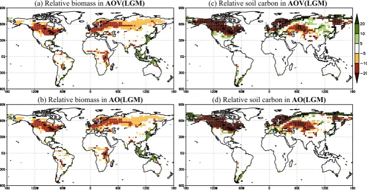
(b) Relative biomass in AO(LGM) (d) Relative soil carbon in AO(LGM) (c) Relative soil carbon in AOV(LGM)

Fig. 7.

Equilibrium absolute differences of biomass [kg/m

2

] in (a)

AOV(LGM)

and (b)

AO(LGM)

with respect to

AOV(PI)

. Equilibrium absolute differences of soil carbon [kg/m

2

]

in (d)

AOV(LGM)

and (d)

AO(LGM)

with respect to

AOV(PI)

. Absolute values are shown in

Appendix Figure A2.

42

Fig. 7. Equilibrium absolute differences of biomass [kg m−2] in (a) AOV(LGM) and (b) AO(LGM) with respect to AOV(PI). Equilibrium absolute differences of soil carbon [kg m−2] in (c) AOV(LGM) and (d) AO(LGM) with respect to AOV(PI). Absolute values are shown in the Appendix Fig. A2.

also a decrease of biomass. Other forest areas also show a decrease in biomass which is consistent with the decrease of NPP (Fig. 3h) , but typically less than 5 kgC m−2. The largest decrease of soil carbon is seen in East Siberia and Central Eurasia (Fig. 7c), which corresponds to the replacement of boreal forest by tundra and desert, respectively. This can be explained by the decrease of NPP (Fig. 3h) which also shows the largest decrease in these areas. In these areas, reduction of NPP causes less input to soil carbon pools so that equi-librium soil carbon decreases. Increase of soil carbon is seen in northeast China, northern Siberia and the southern edge of ice sheets in both Europe and North America. This increase

of soil carbon is due to lowering of decomposition rate of soil carbon, which corresponds to carbon output from terrestrial ecosystem, due to low temperature in the LGM. Other cir-cumstantial evidence is shown in change of NPP (Fig. 3h), which is regarded as carbon input to terrestrial ecosystem. Change of soil carbon does not show increase in all these re-gions. In other regions, the soil carbon shows a slight change, less than±5 kgC m−2.

(12)

1582 R. O’ishi and A. Abe-Ouchi: Climate and vegetation/carbon change in the LGM

in the edge of the tree line (biomass) and in the wide area of the Northern Hemisphere continent (soil carbon). These dif-ferences reflect the changes in habitable zones (biomass) and cooling (soil carbon) due to vegetation-climate feedback.

Offline LPJ-DGVM experiments show biomass response in the LGM (except for new land and preindustrial ice sheet area) to temperature, precipitation and CO2(almost additive)

as well as NPP. On the other hand, soil carbon is not additive (Table 3).

5 Discussion

5.1 Vegetation change and amplification of cooling

In the present study, our results indicate a cooler and drier climate than is shown in previous studies (Braconnot et al., 2007; Crucifix and Hewitt, 2005; Henrot et al., 2009). Com-pared to the latest reconstruction (Bartlein et al., 2011), cool-ing durcool-ing the LGM is overestimated in both North America and Europe. On the other hand, cooling is underestimated in southern Africa. The pattern of precipitation change is generally the same as the reconstruction in North America and Europe, but the intensity of change is underestimated. Since there is relatively less vegetation in these regions and not a major part of terrestrial carbon storage, the influence of climate difference on biomass and soil carbon is limited. We also obtained similar vegetation changes, such as expan-sion of tundra, a southward shift of boreal forests, and ex-pansion of desert/arid regions, compared to previous stud-ies (Prentice and Jolly, 2000; Harrison and Prentice, 2003; Crucifix et al., 2005b; Jahn et al., 2005; Henrot et al., 2009; Prentice et al., 2011). The resultant vegetation-climate feed-back is positive, which has been shown in previous sensitiv-ity studies (Ganopolski, 2003; Crucifix et al., 2005a; Henrot et al., 2009).

In the present study, the most dominant factor in the vegetation-climate model results is the increase in land sur-face albedo (Fig. 5a), which is due not only to the replace-ment of boreal forest by tundra and desert, but also to the in-crease in snow cover (Fig. 5b) in mid-latitudes, in spite of the reduction in precipitation (Fig. 4d). Generally, the cooling in surface temperature is dominated by reduction of sensible heat from land (Fig. 6c). This sensible heat balance shows a very similar pattern to that of surface shortwave balance (Fig. 6a) which is directly related to surface albedo (Fig. 5a). We obtained−1.55 W m−2 _{of clear sky surface shortwave}

forcing which is shown as−1.4 W m−2_{by Crucifix and}

He-witt (2005). Surface longwave balance (Fig. 6b) and surface latent heat balance (Fig. 6d) do not explain the sensible heat balance (Fig. 6c) induced by vegetation change. In high lati-tudes, snow cover shows a slight decrease (Fig. 5b), and thus decreases the albedo (Fig. 5a) due to the reduction of pre-cipitation (Fig. 4) which reflects weakening of global water cycle due to cooling induced by vegetation change.

The MIROC-LPJ predicts a boreal forest band in west-ern Siberia that is not seen in previous model studies using GCMs and vegetation models (Harrison and Prentice, 2003; Crucifix et al., 2005b; Prentice et al., 2011). In those stud-ies, the boreal forest on the Eurasian continent is separated into east and west sections, or vanished completely. There are three possible explanations for this overestimation of bo-real forest. First, the MIROC-LPJ shows a weaker cooling in western Siberia than do the PMIP2 model results (Braconnot et al., 2007). This weak cooling is not due to the positive vegetation-climate feedback in AOV(LGM) because the of-fline LPJ-DGVM run, using the result of the AO(LGM), pre-dicts the same vegetation in this region (not shown). The sec-ond reason is related to the lack of fractional coverage repre-sentation in the land-surface scheme of the MIROC-LPJ. As described in Sect. 2.3 and O’ishi and Abe-Ouchi (2009), the land-surface scheme of the MIROC is able to handle only one vegetation type in a grid cell, and so it does not handle frac-tional coverage. We defined the representations of the vegeta-tion types by using combinavegeta-tion of individual fracvegeta-tional cov-erage of PFTs, NPP, LAI, GDD and soil moisture calculated in the coupled LPJ-DGVM. However, there can be an over-estimation of a specific vegetation type which is typically the most dominant vegetation type. In AOV(LGM) in the present study, forest coverage in western Siberia was about 0.6, which was less than that of AOV(PI). However, this for-est is assumed to occupy a whole grid cell in the land-surface scheme of the MIROC. Thus this treatment underestimates both the decrease in forest and the cooling due to vegetation feedback. If we could introduce the fractional representation into the land-surface scheme of MIROC, reduction of forest and increase of tundra cause additional cooling in western Siberia as well as in northeastern China and central Eura-sia. The third reason is model bias of LPJ-DGVM itself. In AOV(PI), a PFT named “boreal needle-leaved summergreen trees” is overestimated even if we apply a bias correction. This tendency of overestimation may also cause overestima-tion of this PFT, which is the most dominant in the boreal forest band in AOV(LGM). The improvement of the produc-tivity of boreal needle-leaved summergreen trees in preindus-trial or present-day simulations may reduce forest band in the LGM simulation.

5.2 Carbon storage

(13)

climate and CO2, washout by ice-sheet coverage, and new

stock on the exposed continental shelf.

Response of terrestrial biosphere to the cool, dry, and low-CO2LGM environment is seen in the reasonable reduction of

the NPP (Fig. 3h), biomass (Fig. 7a) and vegetation coverage (Fig. 1c and d), as well as in previous studies. The contribu-tion of temperature, precipitacontribu-tion and CO2level in the LGM

to reduction of global total biomass is almost additive (see

T,CandP in Table 3) as same as that of NPP. On the other hand, summing contributions of these factors to global to-tal soil carbon does not explain the global toto-tal soil carbon reduction in AOV(LGM). Since the response of biomass is additive, the response of total dead biomass as input to soil carbon is also considered to be additive. A possible expla-nation is non-linear relation of temperature and decomposi-tion speed and soil carbon (Lloyd and Taylor, 1994) and non-linear dependency of decomposition speed and soil carbon to soil moisture which is related to temperature and precipita-tion (Foley, 1995) in LPJ-DGVM.

During the LGM, the assumption of washout by the ice sheet may overestimate the reduction of terrestrial carbon, because the carbon flux and storage in the present-day that are predicted by the LPJ-DGVM tend to be larger than the typical values (Sitch et al., 2003; Denman et al., 2007) and those among multi-models (Cramer et al., 2001). The sec-ond reason is we do not know how much carbon was stored below an ice sheet during the LGM. We assumed all carbon is removed by the ice sheet, which has also been assumed in previous studies. In this case, carbon washout depends on how much carbon was stored in the preindustrial control experiment. On the contrary, the Glacial Burial Hypothesis (Zeng, 2003, 2007) suggests that 500 PgC was buried under the LGM ice sheets. This value is comparable to a decrease of 383 PgC, which we assumed to have been removed by the ice sheets. However,δ13C reconstruction indicates that CO2

rise during the last deglaciation is not from land but from ocean (Lourantou et al., 2010), which is consistent to our assumption of washout.

Since we use a sea level change of −150 m, which is the largest estimation (Yokoyama et al., 2000), the exposed ice-free continental shelf was maximized. In our model set-ting, the total area of exposed ice-free continental shelf is 23×1012m2, which is two times larger than that of previ-ous studies (Zeng, 2003; Montenegro et al., 2006). If we as-sume a more moderate sea level change, such as that noted in Montenegro et al. (2006), the increase of terrestrial carbon (293 PgC) is reduced by about half (which is roughly esti-mated proportionally to the area of ice-free continental shelf) and falls into the range of previous studies (112–323 PgC).

The impact of using the AOGCM results instead of the AOVGCM results is far smaller than the total amount of veg-etation, soil, and total carbon storage during the LGM (less than±20 PgC out of several 1000 PgC; see Table 3) and does not change the main result in the present study. However, these differences are non-negligible if we try to explain the

100 ppm difference of atmospheric CO2 concentration

be-tween the LGM and the preindustrial era, which corresponds to 200 PgC.

6 Conclusions

In the present study we apply a coupled atmosphere-ocean-vegetation GCM for predicting the LGM climate and vegeta-tion in order to quantify how the vegetavegeta-tion-climate feedback affected the LGM climate. Our sensitivity experiments show tendencies similar to previous paleodata and paleomodeling studies for changes in vegetation and climate. In the present study, vegetation changes during the LGM amplify cooling during the LGM by 13.5%, which is mostly caused by in-creases of the land surface albedo. We separate the LGM en-vironment changes into three factors: temperature, precipi-tation, and CO2. We then investigate the impact of each of

these on the vegetation distribution during the LGM. Offline sensitivity experiments indicate that temperature and precip-itation are dominant in the vegetation distribution during the LGM. Low levels of CO2during the LGM affects only the

tropical regions.

We also investigate terrestrial carbon storage during the LGM by offline dynamical vegetation model experiments. Temperature, precipitation (predicted by GCM experiment) and atmospheric CO2 levels of GCM experiments are used

as forcing. The results show that terrestrial carbon storage is generally the same, both in pattern and quantity, regardless of whether we include vegetation-climate feedback in the in-put variables. However, the difference is comparable to car-bon quantity, which corresponds to the 100 ppm of CO2

dif-ference between the LGM and the preindustrial era. We de-termine that inclusion of vegetation-climate feedback should be taken into account if we wish to explain the lowering of atmospheric CO2during the LGM.

We separate the terrestrial carbon difference between the LGM and preindustrial era into three factors: response to the LGM climate and CO2, washout by ice-sheet coverage, and

(14)

1584 R. O’ishi and A. Abe-Ouchi: Climate and vegetation/carbon change in the LGM

of variability among previous studies if we assumed the same area as did previous studies.

Our result in the present study is done by just one model. Since our model tends to overestimate terrestrial carbon storage compared to previous studies (Cramer et al., 2001; Denman et al., 2007; Ciais et al., 2011; Prentice et al., 2011), reduction of terrestrial carbon in the LGM climate is consid-erably larger in range of uncertainty (Bird et al., 1994). We also assumed the largest extent of the continental shelf so that the new storage on the continental shelf is maximized. Our model is considered to overestimate response (both pos-itive and negative) of carbon storage in the LGM than pre-vious model studies. Our result indicates that total terrestrial carbon response in the LGM is calculated by various factors of terrestrial carbon change (ice sheet washout, new storage on continental shelf, response of photosynthesis and vegeta-tion feedback to LGM climate). It is not yet clear where the 200 PgC is stored; it corresponds to a decrease of 100 ppm of atmospheric CO2during the LGM (Lourantou et al., 2010;

Ciais et al., 2011; Shakun et al., 2012). When we try to de-termine the global allocation of carbon in the earth system (atmosphere, ocean and land) during the LGM, we find that not only the uncertainty of photosynthesis response but also vegetation-climate feedback and the uncertainty of sea level change should be taken into account. This is a common im-portant problem among other models as well as our model.

Appendix A

Discussion

P

ap

er

|

Discussion

P

ap

er

|

Discussion

P

ap

er

|

Di

scuss

ion

P

ap

er

|

(a) Vegetation index in AOV(PI) w/o bias correction

(b) Vegetation index in AOV(LGM) w/o bias correction

Fig. A1.

As same as Figure1 but without bias corrected (a)

AOV(PI)

and (b)

AOV(LGM)

.

Fig. A1. The same as Fig. 1 but without bias correction (a)

AOV(PI) and (b) AOV(LGM).

Discussion

P

ap

er

|

Discussion

P

ap

er

|

Discussion

P

ap

er

|

Di

scuss

ion

P

ap

er

|

(a) Biomass in AOV(PI)

(b) Biomass in AOV(LGM)

(c) Biomass in AO(LGM) (f) Soil carbon in AO(LGM)

(e) Soil carbon in AOV(LGM)

(d) Soil carbon in AOV(PI)

Fig. A2.As same as Figure7 but absolute biomass [kg/m2_{] in (a)}_AOV(PI)_{, (b)}_AOV(LGM)_and (c)AO(LGM)and soil carbon [kg/m2_{] in (d)}_AOV(PI)_{, (d)}_AOV(LGM)_and_AO(LGM)_.

44

Fig. A2. The same as Fig. 7 but absolute biomass [kg m−2] in (a) AOV(PI), (b) AOV(LGM) and (c) AO(LGM) and soil carbon [kg m−2] in (d) AOV(PI), (d) AOV(LGM) and AO(LGM).

Acknowledgements. This research is supported by the GRENE

Arctic climate Change Research Project.

Edited by: M. Crucifix

References

Abe-Ouchi, A., Segawa, T., and Saito, F.: Climatic Conditions for modelling the Northern Hemisphere ice sheets throughout the ice age cycle, Clim. Past, 3, 423–438, doi:10.5194/cp-3-423-2007, 2007.

Bartlein, P. J., Harrison, S. P., Brewer, S., Connor, S., Davis, B. A. S., Gajewski, K., Guiot, J., Harrison-Prentice, T. I., Hender-son, A., O., Peyron, A. H., Prentice, I. C., Scholze, M., Seppa, H., Shuman, B., Sugita, S., Thompson, R. S., Viau, A. E., Williams, J., and Wu, H.: Pollen-based continental climate reconstructions at 6 and 21 ka: a global synthesis, Clim. Dynam., 37, 775–802, 2011.

Bird, M. I., Lloyd, J. L., and Farquhar, G. D.: Terrestrial carbon storage at the LGM, Nature, 371, 566–566, 1994.

Braconnot, P., Otto-Bliesner, B., Harrison, S., Joussaume, S., Pe-terchmitt, J.-Y., Abe-Ouchi, A., Crucifix, M., Driesschaert, E., Fichefet, Th., Hewitt, C. D., Kageyama, M., Kitoh, A., Laˆın´e, A., Loutre, M.-F., Marti, O., Merkel, U., Ramstein, G., Valdes, P., Weber, S. L., Yu, Y., and Zhao, Y.: Results of PMIP2 coupled simulations of the Mid-Holocene and Last Glacial Maximum – Part 1: experiments and large-scale features, Clim. Past, 3, 261– 277, doi:10.5194/cp-3-261-2007, 2007.

Ciais, P., Tagliabue, A., Cuntz, M., Bopp, L., Scholze, M., Hoff-mann, G., Lourantou, A., Harrison, S. P., Prentice, I. C., Kel-ley, D. I., Koven, C., and Piao, S. L.: Large inert carbon pool in the terrestrial biosphere during the Last Glacial Maximum, Nat. Geosci., 5, 74–79, 2011.

(15)

R. O’ishi and A. Abe-Ouchi: Climate and vegetation/carbon change in the LGM 1585

CLIMAP Project Members: The Surface of the Ice-Age Earth, Sci-ence, 191, 1131–1137, 1976.

CLIMAP Project Members: The Last Interglasial Ocean, Quar-ternary Res., 21, 123–224, 1984.

Cramer, W., Bondeau, A., Woodward, F. I., Prentice, I. C., Betts, R. A., Brovkin, V., Cox, P. M., Fisher, V., Foley, J. A., Friend, A. D., Kucharik, C., Lomas, M. R., Ramankutty, N., Sitch, S., Smith, B., White, A., and Young-Molling, C.: Global response of terrestrial ecosystem structure and function to CO2and

cli-mate change: results from six dynamic global vegetation models, Global Change Biol., 7, 357–373, 2001.

Crucifix, M. and Hewitt, C. D.: Impact of vegetation changes on the dynamics of the atmosphere at the Last Glacial Maximum, Clim. Dynam., 25, 447–459, 2005.

Crucifix, M., Betts, R. A., and Cox, P. M.: Vegetation and climate variability: a GCM modelling study, Clim. Dynam., 24, 457–467, 2005a.

Crucifix, M., Betts, R. A., and Hewitt, C. D.: Pre-industrial-potential and Last Glacial Maximum global vegetation simulated with a coupled climate-bio sphere model: Diagnosis of biocli-matic relationships, Global Planet. Change, 45, 295–312, 2005b. Denman, K. L., Brasseur, G., Chidthaisong, A., Ciais, P., Cox, P. M., Dickinson, R. E., Hauglustaine, D., Heinze, C., Holland, E., Ja-cob, D., Lohmann, U., Ramachandran, S., daSilbaDias, P. L., Wofsy, S. C., and Zhang, X.: Coupling Between Changes in the Climate System and Biogeochemistry. In: Climate Change 2007 The Physical Science Basis: Contribution of working Groupe I to the Fourth Assesment Report of the Intergovernmental Panel on Climate Change, edited by: Solomon, S., Qin, D., Manning, M., Chen, Z., Marquis, M., Averyt, K. B., Tignor, M., and Miller, H. L., Cambridge University Press, Cambridge, 2007.

Ehret, U., Zehe, E., Wulfmeyer, V., Warrach-Sagi, K., and Liebert, J.: HESS Opinions “Should we apply bias correction to global and regional climate model data?”, Hydrol. Earth Syst. Sci., 16, 3391–3404, doi:10.5194/hess-16-3391-2012, 2012.

Enting, I. G.: The incompatibility of ice-core CO2 data with

re-construction of biotic CO2sources (II) – the influence of CO2

-fertilized growth, Tellus B, 44, 23–32, 1992.

Faloon, P. D., Jones, C. D., Ades, M., and Paul, K.: Direct soil moisture controls of future global soil carbon changes; an impor-tant source of uncertainty, Global Biogeochem. Cy., 25, GB3010, doi:10.1029/2010BG003938, 2011.

Falloon, P. D., Dankers, R., Betts, R. A., Jones, C. D., Booth, B. B. B., and Lambert, F. H.: Role of vegetation change in future climate under the A1B scenario and a climate stabilisation sce-nario, using the HadCM3C Earth system model, Biogeosciences, 9, 4739–4756, doi:10.5194/bg-9-4739-2012, 2012.

Faure, H., Adams, J., Debenay, J., Faure-Denard, L., Grants, D., Pirazzoli, P., Thomassin, B., Velichko, A., and Zazo, C.: Car-bon storage and continental land surface change since the Last Glacial Maximum, Quarternary Sci. Rev., 15, 843–849, 1996. Foley, J. A.: An equilibrium-model of the terrestrial carbon budget,

Tellus B, 47, 310–319, 1995.

Franc¸ois, L. M., Delier, C., Warnant, P., and Munhoven, G.: Mod-elling the glacial-interglacial changes in the continental bio-sphere, Global Planet. Change, 17, 37–52, 1998.

Franc¸ois, L. M., Godderis, Y., Warnant, P., Ramstein, G., de Noble, N., and Lorenz, N.: Carbon stocks and isotopic budgets of the terrestrial biosphere at mid-Holocene and last glacial maximum

times, Chem. Geol., 159, 163–189, 1999.

Friedlingstein, P., Prentice, K. C., Fung, I. Y., John, J. G., and Brasseur, G. P.: Carbon-biosphere-climate interactions in the last glacial maximum climate, J. Geophys. Res., 100, 7203–7221, 1995.

Ganopolski, A.: Glacial integrative modelling, Philos. T. Roy. Soc., 361, 1871–1884, doi:10.1098/rsta.2003.1246, 2003.

Gerber, S., Joos, F., and Prentice, I. C.: Sensitivity of a dynamic global vegetation model to climate and atmospheric CO2, Glob.

Change Biol., 10, 1223–1239, 2004.

Hagemann, S., Chan, C., Hearter, J. O., Heinke, J., Gerten, D., and Piani, C.: Impact of a Statistical Bias Correction on the Projected Hydrological Changes Obtained from Three GCMs and Two Hydrology Models, J. Hydrometeorol., 12, 556–578, doi:10.1175/2011JHM1336.1, 2011.

Harrison, S. P. and Prentice, I. C.: Climate and CO2controls on

global vegetation distribution at the last glacial maximum: analy-sis based on palaeovegetation data, biome modelling and palaeo-climate simulations, Glob. Change Biol., 9, 983–1004, 2003. Hasumi, H.: CCSR Ocean Component Model (COCO),

ver-sion 4.0, center for Climate System Research Report 25, 103 pp., available at: http://www.ccsr.u-tokyo.ac.jp/∼_hasumi/

COCO/coco4.pdf, 2006.

Hasumi, H. and Emori, S.: K-1 Coupled GCM (MIROC) Descrip-tion, k-1 Technical Report No. 1, Center for Climate System Research (CCSR, Univ. of Tokyo), National Institute for Envi-ronmental Studies (NIES), Frontier Research Center for Global Change (FRCGC), 2004.

Henrot, A.-J., Franc¸ois, L., Brewer, S., and Munhoven, G.: Im-pacts of land surface properties and atmospheric CO2on the Last

Glacial Maximum climate: a factor separation analysis, Clim. Past, 5, 183–202, doi:10.5194/cp-5-183-2009, 2009.

Jahn, A., Claussen, M., Ganopolski, A., and Brovkin, V.: Quantify-ing the effect of vegetation dynamics on the climate of the Last Glacial Maximum, Clim. Past, 1, 1–7, doi:10.5194/cp-1-1-2005, 2005.

Jones, C., McConnell, C., Coleman, K., Cox, P., Faloon, P., Jenkin-son, D., and PowlJenkin-son, D.: Global climate change and soil carbon stocks; predictions from two contrasting modelsfor the turnover of organic carbon in soil, Glob. Change Biol., 11, 154–166, doi:10.1111/j.1365-2486.2004.00885.x, 2004.

Joos, F., Gerber, S., Prentice, I. C., Otto-Bliesner, B. L., and Valdes, P. J.: Transient simulations of Holocene atmo-spheric carbon dioxide and terrestrial carbon since the Last Glacial Maximum, Global Biogeochem. Cy., 18, GB2002, doi:10.1029/2003GB002156, 2004.

Joussaume, S. and Taylor, K. E.: The Paleoclimate Modeling Inter-comparison Project, WCRP 111: Proceedings of the third PMIP Workshop, 2000.

Jouzel, J., Barkov, N. I., Barnola, J. M., Bender, M., Chappellaz, J., Genthon, C., Kotlyakov, V. M., Lipenkov, V., Lorius, C., Petit, J. R., Raynaud, D., Raisbeck, G., Ritz, C., Sowers, T., Stievenard, M., Yiou, F., and Yiou, P.: Extending the Vostok ice-core record of palaeoclimate to the penultimate glacial period, Nature, 364, 407–412, 1993.

(16)

1586 R. O’ishi and A. Abe-Ouchi: Climate and vegetation/carbon change in the LGM

Kohfeld, K. and Harrison, S.: How well can we simulate past cli-mates? Evaluating the models using global palaeoenvironmental datasets, Quaternary Sci. Rev., 19, 321–346, 2000.

K¨ohler, P. and Fischer, H.: Simulating changes in the terrestrial biosphere during the last glacial/interglacial transition, Global Planet. Change, 43, 33–55, 2004.

K¨ohler, P., Joos, F., Gerber, S., and Knutti, P.: Simulated changes in vegetation distribution, land carbon storage, and atmospheric CO2in response to a collapse of the North Atlantic thermohaline

circulation, Clim. Dynam., 25, 689–708, 2005.

Kucera, M., Rosell-Mel´e, A., Schneider, R., Waelbroeck, C., and Weinelt, M.: Multiproxy approach for the reconstruction of the glacial ocean surface (MARGO), Quaternary Sci. Rev., 25, 813– 819, 2005.

Lloyd, J. and Taylor, J. A.: On the temperature-dependent of soil respiration, Funct. Ecol., 8, 315–323, 1994.

Lourantou, A., Lavriˇc, J. V., K¨ohler, P., Barnola, J., Paillard, D., Michel, E., Raynaud, D., and Chappellaz, J.: Constrain of the CO₂rise by new atmospheric carbon isotopic measurements dur-ing the last deglaciation, Global Biogeochem. Cy., 24, GB2015, doi:10.1029/2009GB003545, 2010.

Mahowald, N. M., Muhs, D. R., Levis, S., Rasch, P. J., Yoshioka, M., Zender, C. S., and Luo, C.: Change in atmospheric mineral aerosols in response to climate: Last glacial period, preindustrial, modern, and doubled carbon dioxide climates, J. Geophys. Res., 111, D10202, doi:10.1029/2005JD006653, 2006.

Meehl, G. A., Stocker, T. F., Collins, W. D., Friedlingstein, P., Gaye, A. T., Gregory, J. M., Kitoh, A., Knutti, R., Murphy, J. M., Noda, A., Raper, S. C. B., Watterson, I. G., Weaver, A. J., and Zhao, Z.-C.: Global Climate Projection, in: Climate Change 2007 The Physical Science Basis: Contribution of working Groupe I to the Fourth Assesment Report of the Intergovernmental Panel on Cli-mate Change, edited by: Solomon, S., Qin, D., Manning, M., Chen, Z., Marquis, M., Averyt, K. B., Tignor, M., and Miller, H. L., Cambridge university press, Cambridge, 2007.

Monnin, E., Indermühle, A., Dällenbach, A., Flückiger, J., Stauffer, B., Stocker, T. F., Raynaud, D., and Barnola, J.-M.: Atmospheric CO2Concentrations over the Last Glacial Termination, Science,

291, 112–114, 2001.

Montenegro, A., Eby, M., Kaplan, J. O., Meissner, K. J., and Weaver, A. J.: Carbon storage on exposed continental shelves dur