www.nonlin-processes-geophys.net/21/569/2014/ doi:10.5194/npg-21-569-2014
© Author(s) 2014. CC Attribution 3.0 License.
Nonlinear Processes
in Geophysics
An ETKF approach for initial state and parameter estimation in ice
sheet modelling
B. Bonan1, M. Nodet1,2, C. Ritz3, and V. Peyaud3
1INRIA, Laboratoire Jean Kuntzmann (LJK), Grenoble, France
2Université Joseph Fourier Grenoble I (UJF), Laboratoire Jean Kuntzmann (LJK), Grenoble, France
3UJF – Grenoble 1/CNRS, Laboratoire de Glaciologie et Géophysique de l’Environnement (LGGE) UMR5183,
Grenoble, 38041, France
Correspondence to: M. Nodet ([email protected])
Received: 2 July 2013 – Revised: 18 February 2014 – Accepted: 5 March 2014 – Published: 25 April 2014
Abstract. Estimating the contribution of Antarctica and Greenland to sea-level rise is a hot topic in glaciology. Good estimates rely on our ability to run a precisely calibrated ice sheet evolution model starting from a reliable initial state. Data assimilation aims to provide an answer to this problem by combining the model equations with observations. In this paper we aim to study a state-of-the-art ensemble Kalman filter (ETKF) to address this problem. This method is imple-mented and validated in the twin experiments framework for a shallow ice flowline model of ice dynamics. The results are very encouraging, as they show a good convergence of the ETKF (with localisation and inflation), even for small-sized ensembles.
1 Introduction
Antarctica and Greenland account for a significant fraction of today’s sea-level rise (Shepherd et al., 2012). Good esti-mates of their future contribution are therefore crucial to pro-ducing sea-level change forecasts, as underlined by Hanna et al. (2013). Producing pertinent estimates of polar ice sheet contribution to sea-level change relies on our ability to run a precisely calibrated ice sheet evolution model starting from a reliable initial state. Calibrating the model means identi-fying as best we can the unknown parameters of the model (bedrock topography, basal friction law), and finding a reli-able initial state means of identifying the model varireli-ables that vary in time (ice thickness).
In this work we will not address calibration of the full comprehensive model. Indeed, this problem covers a wide range of research fields: numerical analysis, mass-balance
modelling, thermo-mechanical modelling. We will address the problem of initial state and parameter estimation. There exists a wide range of methods to solve this problem, all of them looking to produce a good fit between the estimated present state and the available observations.
There is a variety of models dealing with ice flow; all of them are based on the quasi-static equilibrium equation and consider ice as a viscous fluid with a nonlinear viscosity. Most models take advantage of the very small aspect ratio of ice sheets and use a thin layer approximation, but they differ on the order of the approximation. We use here the simplest approximation (shallow ice approximation). Although sim-ple and fast, it preserves the nonlinearity of the system and is sensitive to the parameters we want to estimate, bedrock elevation and basal drag.
Griggs and Bamber (2009). Ice velocity is obtained by radar interferometry and maps are available over the major part of both ice sheets with a kilometric resolution (Rignot et al., 2011 for Antarctica, Joughin et al., 2010 for Greenland). The uncertainty ranges from 1 to 17 m per year (Rignot et al., 2011). Beside satellite observations, there are also localised measurements of the bedrock topography generally obtained by radar measurements from planes and thus restricted to flight lines. A bedrock topography map has been recently published gathering all the measurements from any country (Fretwell et al., 2013). The coverage is however still hetero-geneous, from closely spaced flight lines in some places to huge regions with no flight at all. The map comes thus with an associated error map, ranging from 20 m (on measured points) up to 1000 m (in unobserved areas), and it is worth noting that this error map is obtained thanks to the kriging method, with no ice flow consideration.
Data assimilation (DA) covers the methods used to com-bine model and data in order to estimate initial states or pa-rameters. There are two main classes of DA algorithms: vari-ational, based on optimal control theory (the prototype being 4D-Var), and sequential, based on optimal statistical estima-tion (the prototype being the Kalman filter). DA is widely known in weather and oceanography forecasting, but its in-troduction in glaciology is fairly recent, in particular for the initial state estimation problem for sea-level rise. MacAyeal (1992) and MacAyeal (1993) introduced control methods to infer basal drag in ice-stream models, using in particular the self-adjoint property of such models, leading to many appli-cation papers (Rommelaere and MacAyeal, 1997; Vieli and Payne, 2003), and later for full Stokes models (Morlighem et al., 2010; Jay-Allemand et al., 2011). Later on, many DA and inverse methods were introduced in glaciology. The Best Linear Unbiased Estimation (BLUE) and Optimal In-terpolation (OI) methods were introduced by Arthern (2003) and Berliner et al. (2008). The Robin inverse method due to Chaabane and Jaoua (1999) has been introduced by Arthern and Gudmundsson (2010) for ice sheet models, and finally, Heimbach and Bugnion (2009) presented the first adjoint ice sheet model derived automatically.
As the ice surface elevation is pretty well (in terms of ac-curacy and data density) observed by satellite sensing, ini-tial state estimation focuses on bedrock topography and basal sliding law estimation. The joint identification of bedrock to-pography and basal friction law is a difficult problem. In-deed, different configurations (e.g. a low bed and no sliding versus a higher bed with sliding) may lead to identical sur-face observations. This is why most of the previous works on this subject chose to investigate the basal sliding iden-tification only, usually for local modelling (glaciers or ice streams). Recently, a couple of papers addressed the ice-sheet initialisation problem: Arthern and Hindmarsh (2006) with a BLUE/OI method and Gillet-Chaulet et al. (2012) with con-trol and Robin methods. More recently still, researchers have started to investigate coupled inversion of bedrock
topogra-phy and basal drag simultaneously; see Raymond-Pralong and Gudmundsson (2011) (using the Bayes theorem) and van Pelt et al. (2013) (with a simple Picard iteration to reduce the observation–model misfit). In the slightly different con-text of calibrating climatic parameters used by an ice sheet model, Tarasov et al. (2012) use a more general approach called Markov Chain–Monte Carlo using neural networks. Contrary to the variational approach or Kalman, this Monte Carlo approach solves the Bayes theorem exactly, which is the basis of every DA system. However, this method cannot be applied in our context due to the too high dimension of the problem: Tarasov et al. (2012) needed over 50 000 runs of their model in order to estimate accurately the statistics of 39 parameters.
Variational and Kalman DA methods are equivalent un-der the condition of linearity, in which they achieve least-variance linear estimation. If in addition errors are Gaussian, they achieve Bayesian estimation. Of course in the frame-work of realistic applications, models are seldom linear and errors are not Gaussian, so that both methods have different advantages and drawbacks, and may compare differently de-pending on the application. In this paper we made the choice to start our investigation with a Kalman-based method. The Kalman filter (KF) was introduced by Kalman (1960) for linear systems. Later on it was extended to nonlinear sys-tems. Because of the curse of dimensionality the extended Kalman filter is not practical in large realistic systems, as the size of the state vector prevents the computation of the time-evolving covariances. Evensen (1994) then introduced the ensemble Kalman filter (EnKF), which is a Monte Carlo approximation of the KF that avoids the computation of the covariance matrices. Following the corrected version of the algorithm by Burgers et al. (1998), numerous authors used the EnKF and proposed improvements and variants.
To the best of our knowledge, neither KF nor EnKF has ever been used in glaciology, and we propose to implement and investigate its performance to tackle the sea-level rise problem. This paper is organised as follows: in Sect. 2 we give some details about the DA methods, in Sect. 3 we de-scribe the ice-sheet model and in Sect. 4 we dede-scribe our nu-merical results. Finally we discuss the results and conclude in Sect. 5.
2 Methods
First introduced by Evensen (1994) and later corrected by Burgers et al. (1998), the ensemble Kalman filter (EnKF) is a common approach in data assimilation for state and param-eter estimation. In the traditional Kalman filter, the state of a physical system at a timetk is represented by two
quan-tities:xk, the augmented state vector of sizenx which
con-tains an estimation of all variables and parameters we wish to estimate, and Pk, the error covariance matrix of this
quantities by the use of an ensemble ofNe realisationsx(i)k ,
i=1, . . . , Ne. The estimation of the extended state vector is
given by the ensemble mean
xk=
1
Ne
Ne X
i=1
x(i)k (1)
and Pkby the ensemble covariance matrix
Pk=
1
Ne−1
XkXkT, (2)
with Xk= h
x(k1)−xk, . . . ,x(Ne)k −xk i
the ensemble pertur-bation matrix.
EnKF is a two-step algorithm: forecast and analysis. Quantities produced during the forecast step (analysis step) are denoted with a superscriptf(superscripta).
The forecast consists in propagating the ensemble using a numerical model:
x(i)k f=Mk
x(i)k−1a+η(i)k , (3)
withMk a nonlinear model which propagates the state
vec-tor from timetk−1to timetk (of course, the model does not
change the parameters) andη(i)k a sample vector following the model error pdf. In this paper we assume a perfect model so thatη(i)k =0.
At timetkobservations are available. We denote them yok,
which is a vector of sizeny. The mapping between
observa-tions and model state is given by the following relation: yok=Hk xtk
+k (4)
withHk a possibly nonlinear observation operator, xt k the
true extended model state vector andkthe observation error. k is assumed unbiased (zero mean) and Gaussian with the
covariance matrix Rk.
The aim of the analysis step is to correct the forecast en-semble thanks to the observations. Several versions of EnKF exist. Here we use a deterministic one called the ensemble transform Kalman filter (ETKF). In the following, we omit the time indexkfor readability.
2.1 ETKF formulation
The ETKF was first introduced by Bishop et al. (2001). The main idea of this formulation is the following: the analysis covariance matrix Pa can be written as a transformation of the forecast ensemble perturbations as
Pa=XfePaXf T
, (5)
withePaanNebyNematrix. The same idea (in a slightly
dif-ferent formulation) was developed for the SEIK filter (Pham, 1996; Pham et al., 1998; Pham, 2001). Here we follow the
ETKF implementation given by Hunt et al. (2007). In order to formulate the analysis step, we first define the forecast en-semble projected in observation space as follows,
n
y(1)f=Hx(1)f, . . . ,y(Ne)f=Hx(Ne)fo, (6) and we denote yfthe mean of the above ensemble and Yfthe associated perturbation matrix. The analysis step then con-sists in minimising the following cost function:
J(w)=Ne−1
2 w
Tw
+1
2
yo−yf−YfwTR−1yo−yf−Yfw, (7) wherewis a vector of sizeNe. The minimiser ofJ is given
by
wa=ePaYf T
R−1yo−yf, (8)
where
ePa=
YfTR−1Yf+(Ne−1)I
−1
(9) is the inverse of the Hessian ofJ at the minimum. The en-semble covariances after the analysis are given by Eq. (5) and the ensemble mean by
xa=xf+Xfwa. (10)
The analysis ensemble perturbation matrix is obtained by Xa=Xf (Ne−1)ePa
1/2
U, (11)
where U is an arbitrary orthogonal matrix which preserves the ensemble mean. For the sake of simplicity, we set U as the identity matrix in the sequel.
Using Eqs. (10) and (11) we can then proceed to the next forecast step using Eq. (3).
2.2 Inflation and ETKF
EnKF is known for suffering from under-sampling issues (the so-called curse of dimensionality). Two well-known proce-dures have been developed to correct their symptoms: infla-tion and localisainfla-tion. The former scales up by a factor the ensemble perturbation matrix to avoid the underestimation of the variances (Anderson and Anderson, 1999). The scal-ing factor is also known as the forgettscal-ing factor in Pham et al. (1996). In the ETKF formulation of Hunt et al. (2007), the inflation consists in replacing Eq. (9) by
ePa=
YfTR−1Yf+Ne−1
ρ I
−1
, (12)
0 200 400 600 800 1000 1200 −1000
0 1000 2000 3000
xaxis (in km)
altitude (in m)
B
soc: Bedrock topography H: Ice thickness S: Surface
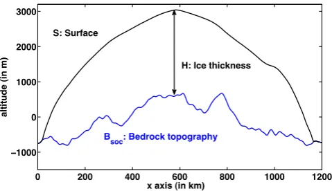
Fig. 1. Ice sheet geometry: an ice cap of thicknessH (x, t )lies on a bedrock (in blue) whose topography isBsoc(x).S(x, t )represents
the surface altitude of the ice sheet.
2.3 Localisation and ETKF
Another under-sampling issue of EnKF is the problem of long-range spurious correlations. These can be overcome by the use of localisation. The ETKF configuration in Hunt et al. (2007) does not allow the use of localisation on a fore-cast error covariance matrix as in Hamill et al. (2001) or Houtekamer and Mitchell (2001). However, localisation on R is still possible. One way is to perform local analysis by assimilating a subset of observations on a given location (Ott et al., 2004). It has been implemented by Hunt et al. (2007) and is known as LETKF. This method can lead to disconti-nuities in the analysis when an observation leaves the sub-set of used observations for a given location. To solve this, Hunt et al. (2007) select a subset of observations and in-crease error variance for observations close to the boundary of the subset. It is equivalent for a given location to replace R withρ−l1◦R, withρlsome distance-based correlation matrix
(such as the one suggested by Gaspari and Cohn, 1999), the origin being the given location and◦denoting the element-wise (Hadamard or Schur) product. Note thatρ−l 1◦R must be changed for each given location even if it uses the same observations as for another location. We use this corrected version of LETKF for our experiments.
Note that (L)ETKF can produce negative ice thicknesses. In those (rare) cases, we set back ice thickness to zero.
3 Ice sheet model
3.1 Basis of ice sheet model
The goal of an ice sheet model is to simulate the evolution of ice thicknessH (x, t )over a supposedly fixed bedrock to-pographyBsoc(x)(Fig. 1). The total has a surface elevation
denotedS(x, t ), according to
S(x, t )=H (x, t )+Bsoc(x), (13)
Table 1. List of parameter values involved in the parameterisation
of the surface mass balance. AsFclimis a time-evolving climatic
pa-rameter, its value will be specified for each experiment in Sect. 4.1.
Parameter Value Abl0 −5 m.a−1
Acc0 6 m a−1 c1 0.115
Tmelt −6◦C
λ 111 0001 ◦C m−1
γ −0.0063◦C m−1
wheret represents the time, and thex axis represents the latitude.
Ice sheet thicknessH (x, t )is governed by the balance be-tween surface mass budget, precipitation or surface melting, and ice flow that drains ice accumulated in the central parts toward the edges of the ice sheet. All these components can evolve with time in response to climatic changes and inter-nal feedbacks. In the context of model initialisation, we will focus on ice flow, surface mass balance being assumed as known.
In this study, we use a parameterisation of surface mass balancebmas a function of atmospheric temperatureTs. The
values of the different parameters involved in this parame-terisation are detailed in Table 1. The surface mass balance is the sum of accumulation Acc≥0 (snowfalls) and Abl≤0 (melting). These two terms are parameterised as follows:
Acc=Acc0e−c1Ts (14)
Abl=
Abl0
Ts−Tmelt
Tmelt 2
if Ts> Tmelt
0 else
(15)
Ablation occurs when the temperature exceeds the melting point, represented byTmelt. The surface temperatureTs
de-pends on surface elevation of the ice sheetS, distance along thexaxis (representing latitude withx=0 the pole) and cli-mate temperatureFclim, according to the formula:
Ts(x, t )=Fclim+λ x+γ S(x, t ) (16)
Fclimevolves in time; its value will be specified for each
ex-periment in Sect. 4.1.
This parameterisation (values are detailed in Table 1) re-produces qualitatively the typical surface mass balance over an ice sheet and the feedbacks associated with its possible changes in geometry.
Ice flow is gravity driven: it follows the quasi static equi-librium equation, i.e. the momentum conservation equation in which the only body force is due to gravity and accelera-tion is negligible.
at the surface snow slowly densifies in firn and ice, this pro-cess is restricted to the top 100 m of the ice sheet (over about 3000 m). Thus, for large-scale modelling, this layer is re-placed by an ice equivalent one with density equal to ice den-sity.
Ice behaves as a viscous fluid with a nonlinear viscosity. It is usual among glaciologists to use the empirical “Glen” flow law (Duval, 1979) with an exponent 3 (see below for more details). In the following however we will use a poly-nomial law associating the Glen flow law and a Newtonian one. This law was suggested by Lliboutry (1993) and Cuffey and Paterson (2010), and can better represent deformation at very low stresses existing for instance in the upper part of the ice sheet. Moreover, it prevents infinite viscosity in the case of no deformation. It is written as:
˙ ij=
1 2
∂u
i ∂xj
+∂uj
∂xi
=Aτ2+φτij0, (17)
where˙ij is the train rate tensor component, ui the
veloc-ity in the directioni,τij0 is the deviatoric stress component,
Aandφ are the coefficients of, respectively, the Glen flaw law (n=3) and the linear (Newtonian) flow law andτ is the effective stress, or formally the second invariant of the devi-atoric stress tensor.
Boundary conditions at the surface are atmospheric pres-sure and no tangential stress. At the ice bed interface, a drag-ging law (usually called sliding law by glaciologists) must be prescribed to derive the tangential stressτb(also called basal
drag).
The dragging law depends on the substratum, and espe-cially on whether it is hard-bed or soft-bed (sediment). How-ever, many of the sliding/dragging laws proposed in glaciol-ogy can be written as follows (see Cuffey and Paterson, 2010):
τb=KUslida , (18)
whereUslid is the basal tangential velocity,K anda are
re-spectively coefficient and exponent of the dragging law and their value depends on the characteristics of the rock–ice in-terface, basal temperature, sediment thickness, water pres-sure, roughness, etc. In this article, we will restrict our work to a linear law (a=1).
Note that when the ice sheet reaches the ocean, ice be-gins to float and forms structures called ice shelves (or float-ing tongues if they are narrow). Basal drag there is zero and Eq. (18) is not valid. In this work we will only consider an ice sheet resting on the bedrock (grounded ice sheet).
Associating quasi static equilibrium and viscous behaviour leads to the full Stokes equations. There is a whole hier-archy of approaches to solve this problem (see for instance the ISMIP inter-comparison project, Pattyn et al., 2008). Re-cently, a few ice sheet models were designed to solving rig-orously the full Stokes problem, but given the numerical cost they are usually restricted to a regional scale or can only
afford a few century simulations; see Gillet-Chaulet et al. (2012), Larour et al. (2012). All the other ice sheet models use approximations based on the very small aspect ratio of ice sheets. Ice sheets are indeed a few kilometres thick and more than a thousand kilometres wide, so that asymptotic developments are possible. In this work, we will use an ap-proximation called shallow ice apap-proximation that preserves the main nonlinearity of the problem, linked to the deforma-tion law, and the dependency on the dragging law coefficient that is one of the characteristics we want to estimate. 3.2 Shallow ice approximation (SIA) for a flowline
model
This approximation (Hutter, 1983) describes ice deformation in the vertical plane and allows us to calculate the vertical profile of horizontal velocity. It is based on an asymptotic approach and is vertically integrated. We use here a model, Winnie, which is a flowline and isothermal version of a 3-D ice sheet model, GRISLI (see Ritz et al., 2001; Peyaud et al., 2007; Quiquet et al., 2012). According to the SIA, ice flow is in the direction of the steepest slope of the surface and can be thus relatively well represented by a flow line follow-ing that direction. The isothermal assumption allows uniform deformation coefficients,Aandφ(their values are given in Table 2). It is taken as a first step in this study because taking thermal processes into account would require us to estimate a third poorly known parameter that is the geothermal heat flow. Such a topic is beyond the scope of this study.
The vertically averaged horizontal velocity,U, is given by
U=Udef+Uslid. (19)
Udefcomes from ice deformation in the vertical plane, and
according to the SIA equations and our constitutive equation (polynomial) reads as
Udef=
"
−A
5(ρg)
3H4∂S
∂x
2
−φ
3ρgH
2
# ∂S
∂x, (20)
wherexis the horizontal coordinate,ρis ice density,g grav-ity,HandSare ice thickness and ice sheet surface elevation. Note that the nonlinearity of the constitutive equation is implicitly taken into account by the exponents for surface slope and ice thickness.
The horizontal velocity at the surfaceUsis one of the
ob-served characteristics and is given by
Us=
"
−A
4 (ρg)
3H4∂S
∂x
2
−φ
2ρgH
2
# ∂S
∂x+Uslid. (21)
To derive the basal velocityUslid, we assume that basal drag
and basal velocity are linked through a linear dragging law and that the basal shear stressτbis given by the SIA:
τb=ρgH
∂S
Table 2. List of parameter values involved in the computation of ice
velocities.
Parameter Value
ρi 910 kg m−3
g 9.81 m s−2
A 2×10⁻¹⁶Pa−3a−1
φ 8.313 Pa−1a−1
whereβ is positive and is one of the characteristics we want to determine. Because this parameter covers several orders of magnitude, we often useα=log10(β).
The previous equation is one example of the sliding laws described in Eq. (18). Although simple, this method repro-duces the various types of ice flow found in ice sheets: slow flow in the central parts where ice deformation is dominant, and fast flow in ice streams for low values ofβ. Such a sim-ple sliding relation cannot reflect the large variety of slid-ing processes and their nonlinearities, but is sufficient for our purpose, especially with the isothermal assumption (Bueler and Brown, 2009). Moreover, due to the thin layer approxi-mations, one should be careful in the interpretation of sharp horizontal changes in the bedrock topography or basal drag coefficient.
Finally, the evolution of ice sheet geometry is derived from the mass conservation equation:
∂H
∂t =bm−
∂U H
∂x (23)
In our model, mass conservation is the only time-dependent equation andH is the only prognostic variable. Ice veloci-ties are diagnostic (completely determined by the ice sheet geometry) because acceleration terms are neglected. 3.3 Numerics
The velocity field is obtained analytically from Eqs. (19), (20), and (22) as a function of ice thickness and surface slope. The mass conservation equation (23) is solved by a finite dif-ference method with a staggered regular grid, velocities and slopes grid points are taken at the midpoint between thick-ness grid points. Because velocity is strongly dependent on the ice sheet geometry, the time scheme is semi-implicit; see Hindmarsh (2001). We use for every experiment a fixed time step of 0.01 year.
4 Numerical results
We now present our numerical results. This section is divided into four paragraphs: firstly we present the numerical setup of the various experiments. Secondly we explain how to build the initial ensemble members. Thirdly we present the prelim-inary results obtained with the ETKF and a large ensemble.
Finally, we study the impact of smaller ensemble sizes, for ETKF with inflation and localisation.
We recall here that our problem is to estimate jointly the ice thicknessH, the bedrock topographyBsoc, and the basal
sliding coefficientβ=10α. As this particular problem has never been studied before with ensemble filtering, this work is focused on twin experiments, because it will allow quanti-tative assessment of the method performance.
4.1 Numerical setup
Twin experiments consist in comparing three model states: the reference (or true) state, which is used to generate obser-vations; the background state, which is another model state, different from the reference; the assimilated state, also called analysis, resulting from the DA procedure. We can then com-pare the misfit between the assimilation and the reference, and the misfit between the reference and the background (no assimilation).
We performed the twin experiments over a 20-year time window. This is realistic for this problem, as the available observation records roughly span 20 years. Note that this small window size makes our proposed DA experimental setup quite challenging.
We first explain how to choose the reference state. We set up the Winnie model with 241 grid points and a space step
1x=5 km, so that the state vector (H (x), Bsoc(x), α(x))
length is 743. The reference run is initialised att=0, with the ice thicknessH and bedrock topographyBsocpresented
in Fig. 2. This ice thickness is chosen as the stable state for a constant climate forcing (Fclim=8◦C in Eq. 15). In
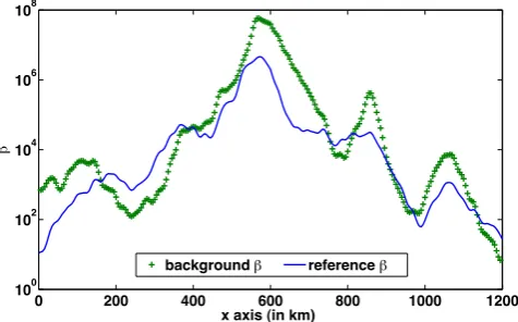
prac-tice, it is produced from a very long (50 000 years) model run, starting fromH=0. Also att=0, the sliding parame-ter coefficientsβ(x)=10α(x)are defined as in Fig. 3.
With this reference initial state, we now impose a linear climate change (+0.2◦C for 20 years, soFclim(t )=8+0.01t
witht in years) and we perform a 20-year model run in or-der to get the reference state over the assimilation window. Note that after 20 years the ice thickness is very similar to the initial one: the dynamics, highly nonlinear, are also very slow.
We then use the reference state to generate synthetic ob-servations. We choose1t=1 year as a realistic observation interval, therefore our assimilation experiments will have 20 observation times, and thus 20 analysis steps. Every year, we observe the surface elevationSand the surface velocity
Usat each grid point (we detailed the reference surface
0 200 400 600 800 1000 1200
−1000 0 1000 2000 3000
xaxis (in km)
altitude (in m)
observed surface background bed reference bed
Fig. 2. Ice sheet geometry for the reference and background states.
Thexaxis represents the horizontal extent of the ice sheet (in km). Theyaxis is the elevation in metres from the sea level. The refer-ence bedrock topography is in blue, the background bedrock is in green crosses. Reference and background surface altitude are iden-tical, in red.
0 200 400 600 800 1000 1200 100
102 104 106 108
xaxis (in km)
!
background ! reference !
Fig. 3. Basal sliding parameterβ(x)as a function of the ice sheet extentx, for the reference state (solid blue) and the background (green crosses), in log scale.
Every DA experiment presented in this section uses the same background state (see Figs. 2 and 3) as an initial en-semble mean. The next section describes how to build the ensemble from the background state. The same process has been used to produce the background state and parameters from the reference.
4.2 Initial ensembles
As we said before, the initial ensemble mean is set to the background state. Before we describe the procedure, we have to acknowledge that some observations were used twice: once to build initial ensembles (i.e. as a priori information), and another time in the DA system (i.e. as observations). This violates a crucial hypothesis required by Kalman-based fil-ters: the independence between the a priori estimation and the observations. However, this is a characteristic of realistic
0 200 400 600 800 1000 1200
−1000
−500 0 500 1000
xaxis (in km)
velocity (in m/yr)
sliding component deformation component surface velocity
Fig. 4. Ice velocity at the surface of the ice sheet for the reference
state, in metres per year, as a function of the ice sheet extentx. The total surface velocityUsis represented in red, its sliding component Uslid is in orange crosses, its deformation componentUs,defwith
cyan x (we recall thatUs=Uslid+Us,def).
frameworks: indeed, the state-of-the-art a priori bedrock to-pography Bedmap2 (Fretwell et al., 2013) is produced using surface altitude observations (as well as all available bedrock measurements).
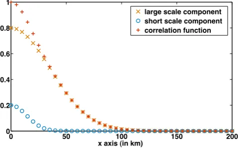
Now let us describe how to build initial ensemble mem-bers. Forβ=10α, we first generate an ensemble ofα(x) pa-rameters drawn from a Gaussian distribution with a given co-variance matrix (a squared exponential coco-variance function). Then we transform this ensemble ofαinto an ensemble ofβ. Then we generate an ensemble of bedrock topographies according to a Gaussian distribution, whose mean is the background and whose covariance matrix is consistent with observation statistics. The covariance matrix requires two ingredients: the variances and a correlation matrix, accord-ing to the formula B=6C6, where 6 is the square root of the diagonal matrix of variances, and C is a correlation matrix. Where bedrock topography observations are avail-able, the variance is set to the observation variance (20 m in standard deviation). Where there is no ice, the variance is set to the surface altitude observation variance (2 m in stan-dard deviation). Elsewhere the variance increases with the distance to the closest observation (bedrock or surface) avail-able. Figure 5 presents the standard deviations that form the diagonal of 6. At worst the standard deviation is equal to 320 m, which is accurate compared to available real uncer-tainty estimation onBsoc.
0 200 400 600 800 1000 1200 0
50 100 150 200 250 300 350
xaxis (in km)
standart deviation (in m)
Fig. 5. Standard deviations (in metres) for the matrix6 used to generate the initial bedrock topography ensembles, as a function of the extentx. Local minimums correspond to either “no ice” points (close to the boundaries of the domain) or observation points.
0 50 100 150 200
0 0.2 0.4 0.6 0.8 1
xaxis (in km)
large scale component short scale component correlation function
Fig. 6. Correlation function (in red crosses) used for the generation
of initial bedrock topography ensembles. This is a combination of two Gaussian functions: one to capture large-scale behaviour (or-ange x) and one for short-scale behaviour (cyan circles).
scale and their slight roughness at shorter scales. This be-haviour seems to produce realistic bedrock topographies.
We now have an ensemble of bedrock topographies. We then generate an ensemble of surface elevations according to a Gaussian distribution. As before, its mean is the true sur-face elevation (from the reference run) and its covariance ma-trix is consistent with surface elevation observation statistics (white noise with a standard deviation of 2 m). To obtain the initial ensemble for ice thickness, we subtract the ensemble of bedrock topography from the ensemble of surface eleva-tion: H=S−Bsoc. Then we correct this new ensemble to
avoid negative ice thicknesses (we just set them back to zero). Finally we run the model for each ensemble member during 1 year in order to obtain more physically balanced ice sheets and we perform a multiplicative rescaling on the produced ensemble so that its mean remains equal to the background. An example of 50 ensemble members is presented in Fig. 7.
0 200 400 600 800 1000 1200
−2000
−1000
0 1000 2000 3000 4000
xaxis (in km)
altitude (in m)
Initial ice sheet ensemble (Ne = 50)
Fig. 7. Example of an initial ice sheet ensemble (50 members):
bedrock topographiesBsoc(x)and surface elevationS(x)as
func-tions of the horizontal distancex.
4.3 First results with a large size of ensemble
We first perform twin experiments with a large ensemble (size Ne=1000) compared to the state vector dimension,
in order to validate our ETKF approach, without having to deal immediately with under-sampling issues. We therefore run the ETKF without inflation or localisation. The bedrock topography obtained after 20 years is presented in Figs. 8 (mean topography with or without assimilation) and 9 (ab-solute difference from the reference with or without assimi-lation). This clearly shows that the final results on ice thick-ness and bedrock topography are very accurate, as the aver-age RMS error for bedrock topography has decreased from 207.5 to 45.9 m and the maximum standard deviation from 671.6 to 150.5 m. The average RMS error for ice thickness has also decreased from 207.5 to 45.5 m and the maximum absolute difference from 671.6 to 150.5 m.
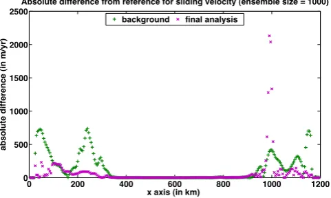
Figure 10 presents the results for theβ parameter. We can see that the accuracy after assimilation is quite good at the edges of the ice sheet and worse in the centre, whereβ is large, and also where there is no ice. However, poor results on largeβ are not meaningful. Indeed, we are mostly inter-ested in recovering the sliding component of the velocity, and it is well known among glaciologists that its sensitivity to variations ofβ for largeβis very low:β≥105leads to zero sliding velocity in any cases, so thatβ=106 or 107 does not make any difference. Similarly, β in areas where there is no ice is meaningless. This is confirmed in Fig. 11, which shows the sliding counterpart of the surface velocity: we can see that the analysis is much closer to the reference than the background. Precisely, Fig. 12 shows the absolute difference from the reference on surface sliding velocity with or without assimilation, and we can see that it is much reduced with as-similation. However,Uslidis poorly retrieved at some points
0 200 400 600 800 1000 1200
−1000
−500 0 500 1000 1500 2000 2500 3000 3500
ETKF result for ice sheet (ensemble size = 1000)
xaxis (in km)
altitude (in m)
observed surface background final analysis reference
Fig. 8. Ice sheet geometries after 20 years, with the 1000-member
ETKF. The analysis bedrock topography (final mean ensemble in purple x) is compared to the background (green crosses) and the ref-erence (blue). The analysis result and the refref-erence are really close except for around 150 km from the origin (see also Fig. 9 for de-tailed results). The surface elevation is accurately observed (in red), so that background, reference and analysis are similar.
0 200 400 600 800 1000 1200
0 100 200 300 400 500 600 700 800
Absolute difference from the reference for bedrock topography (ensemble size = 1000)
x axis (in km)
Absolute difference (in m)
background final analysis
Fig. 9. Absolute difference between analysis and reference (in
pur-ple x) after 20 years of the 1000-member ETKF is compared to the absolute difference between background and reference (in green crosses) for bedrock topography. The average RMS error is de-creased from 207.5 m for the background to 45.9 m for the analysis and the maximum absolute difference from 671.6 to 150.5 m.
the dynamics are close to being discontinuous, and therefore highly nonlinear.
We then apply a slight inflation of 1.01 to the 1000-member ETKF. Figure 13 (to be compared to Fig. 9) shows the improved results for the ice sheet geometry and Fig. 14 (to be compared to Fig. 12) for the sliding velocity. The im-provements due to inflation are particularly pronounced in areas where sliding and deformation are both predominant and the dynamics highly nonlinear.
0 200 400 600 800 1000 1200
10−2
100
102
104
106
108
1010
xaxis (in km)
!
ETKF result for ! (ensemble size = 1000)
background final analysis reference
Fig. 10.βparameter after 20 years of the 1000-member ETKF. The analysis (purple x) is compared to the background (green crosses) and the reference (blue). Values ofβabove 105are all equivalent in terms of sliding velocity. Similarly,βis meaningless where there is no ice (close to boundaries).
0 200 400 600 800 1000 1200
−1500
−1000
−500 0 500 1000 1500 2000 2500 3000
xaxis (in km)
velocity (in m/yr)
ETKF result for sliding velocities (ensemble size = 1000)
background final analysis reference
Fig. 11. Sliding componentUslid of the surface velocity after 20
years of the 1000-member ETKF. The analysis mean (purple x) is compared to the background (green crosses) and the reference (blue).
0 200 400 600 800 1000 1200
0 500 1000 1500 2000 2500
Absolute difference from reference for sliding velocity (ensemble size = 1000)
x axis (in km)
absolute difference (in m/yr)
background final analysis
Fig. 12. Absolute difference between final analysis mean (purple x)
0 200 400 600 800 1000 1200 0
100 200 300 400 500 600 700 800
Absolute difference from reference for bed. topo. (ensemble size = 1000 + inflation 1.01)
xaxis (in km)
Absolute difference (in m)
background final analysis
Fig. 13. Absolute difference between analysis and reference (in
pur-ple x) after 20 years of the 1000-member ETKF with a slight infla-tion of 1.01 is compared to the absolute difference between back-ground and reference (in green crosses) for bedrock topography. The average RMS error (14.0 m) and the maximum absolute differ-ence (47.8 m) are improved compared to the result obtained without inflation.
0 200 400 600 800 1000 1200
0 100 200 300 400 500 600 700 800
Absolute difference from reference for sliding velocity (size = 1000, infla 1.01)
xaxis (in km)
absolute difference (in m/yr)
background final analysis
Fig. 14. Absolute difference between final analysis mean (purple x)
or background (green crosses) and reference sliding component of surface velocity after 20 years of the 1000-member ETKF with a slight inflation of 1.01.
4.4 Dealing with small sizes of ensemble
The results obtained with a large ensemble are satisfying. Nevertheless we will not be able to perform such experiments with a full 3-D large-scale ice sheet model. Indeed, in that case the state vector dimension is larger than 100 000, and it would be impossible to use an ensemble that large. With this remark in mind we now perform ETKF experiments with smaller ensembles: 100, 50, and 30. Without localisa-tion and/or inflalocalisa-tion the ETKF is known for its divergence for small ensembles. To check this fact, we perform one exper-iment with 100 members, without localisation or inflation. Figure 15 presents the final analysed bedrock topography, which is clearly degraded with respect to the background. Actually, RMS error on bedrock topography increases from
0 200 400 600 800 1000 1200
−1000
0 1000 2000 3000 4000
ETKF result for ice sheet (ensemble size = 100)
xaxis (in km)
altitude (in m)
observed surface background final analysis reference
Fig. 15. Bedrock topography after 20 years, with the 100-member
ETKF (no inflation, no localisation). The analysis (final mean en-semble in purple x) is compared to the background (green crosses) and the reference (blue). RMS error increases from 207.5 m for the background state to 302.4 m for the final analysis step and the max-imal absolute difference from 671.6 to 1093.7 m.
0 200 400 600 800 1000 1200
−1000 −500 0 500 1000 1500 2000 2500 3000 3500
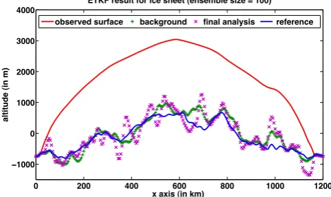
LETKF results for ice sheet (ensemble size = 100, 50, 30)
x−axis (in km)
altitude (in m)
reference background final anal. (100 m.) final anal. (50 m.) final anal. (30 m.) observed surface
Fig. 16. Bedrock topography after 20 years of the LETKF with
in-flation. The background (green) is compared to the reference (blue) and the analyses for various ensemble sizes: 100 members (purple), 50 members (cyan) and 30 members (orange). RMS error evolution is synthesised in Table 3. See also Fig. 17 for detailed results.
207.5 m for the background state to 302.4 m for the final anal-ysis step, which is a 50 % increase.
We then use inflation, as we did with 1000 members. Best results are obtained in that case with an inflation of 1.10. Compared to the results without inflation, RMS er-rors are improved to 121.2 m for the bedrock topography and to 235.4 m year−1 for the sliding velocity; maximum
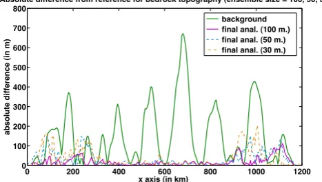
0 200 400 600 800 1000 1200 0
100 200 300 400 500 600 700 800
Absolute difference from reference for bedrock topography (ensemble size = 100, 50, 30)
x axis (in km)
absolute difference (in m)
background final anal. (100 m.) final anal. (50 m.) final anal. (30 m.)
Fig. 17. Absolute difference between results and reference for the
bedrock topography after 20 years of the LETKF with inflation. The background (green) is compared to the analyses for various ensem-ble sizes: 100 members (purple), 50 members (cyan), and 30 mem-bers (orange). RMS error evolution is synthesised in Table 3.
Let us recall briefly how localisation is performed. The observation error covariance matrix R is modified intoρ−l 1◦
R, withρl some distance-based correlation matrix (Gaspari
and Cohn, 1999). The distancel must be tuned manually in order to achieve good results. It corresponds to the maximal distance between a given grid point and the observations used in analysis at this point.
We performed numerous experiments in order to deter-mine by hand the bestl and the best inflation parameter for each ensemble. We chose the bedrock topography RMS er-ror as a score to measure the performance of inflation and localisation. Regarding localisation, the best results were ob-tained withl between 161x (ensemble size 30) and 241x
(ensembles size 50 and 100), so that this distancel is quite insensitive to ensemble sizes. In contrast, the optimal value for the inflation parameter proved to be much more sensitive to ensemble sizes (ranging from 0.98 to 1.14).
Table 3 presents the RMS error and maximal absolute dif-ference from the redif-ference forBsocandUslidfor the optimally
tuned LETFK with 30, 50, and 100 members, as well as the ETKF for 100 and 1000 members. We can see that despite the small ensemble sizes the results are pretty good. Figures 16 and 17 present the bedrock topography and its absolute dif-ference from the redif-ference with 30-, 50-, and 100-member ensembles and confirm the good performance of the filters. As before, the performance onβ itself is not significant, so we show only results on the sliding velocity. Figure 18 shows the sliding velocity, and Fig. 19 presents the absolute differ-ence from the referdiffer-ence for the sliding velocities. As pre-viously, these figures enlighten two different regimes. First, where the ice is either grounded or in full sliding the filters perform quite well. Second, where the ice just starts to slide (where the proportion between the sliding and deformation counterparts of the velocity changes) the filters fail and the RMS is larger, as already noticed in the case of the 1000-member ETKF without inflation.
0 200 400 600 800 1000 1200
−2500 −2000 −1500 −1000 −500 0 500 1000 1500 2000 2500
xaxis (in km)
sliding velocity (in m/yr)
LETKF results for sliding velocity (ensemble size = 100, 50, 30)
reference background final anal. (100 m.) final anal. (50 m.) final anal. (30 m.)
Fig. 18. Sliding componentUslid of the surface velocity after 20
years of the LETKF with inflation. The mean of the final analysis ensemble is compared to the background (green) and the reference (blue), for various ensemble sizes: 100 members (purple), 50 mem-bers (cyan), and 30 memmem-bers (orange). Localisation and inflation parameters are described in Table 3. See also Fig. 19 for detailed results.
0 200 400 600 800 1000 1200
0 500 1000 1500 2000
2500Absolute difference from reference for sliding velocity (ensemble size = 100, 50, 30)
x axis (in km)
absolute difference (in m/yr)
background final anal. (100 m.) final anal. (50 m) final anal. (30 m.)
Fig. 19. Absolute difference between results and reference for the
sliding componentUslid of the surface velocity after 20 years of
the LETKF with inflation. The background (green) is compared to the analyses for various ensemble sizes: 100 members (purple), 50 members (cyan), and 30 members (orange). RMS error evolution is synthesised in Table 3.
We also performed LETFK (with inflation) experiments with smaller ensembles (sizes 10 and 20), but the results were very dissatisfying because of filter divergence (not shown here).
5 Conclusions and further directions
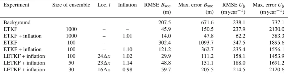
Table 3. Summary of best LETKF + inflation results in term of RMS and maximal absolute difference and comparison with standard ETKF
results.
Experiment Size of ensemble Loc.l Inflation RMSEBsoc Max. errorBsoc RMSEUb Max. errorUb
(m) (m) (m year−1) (m year−1) Background – – – 207.5 671.6 238.1 737.1
ETKF 1000 – – 45.9 150.5 237.9 2130.0
ETKF + inflation 1000 – 1.01 14.0 47.8 62.2 383.3
ETKF 100 – – 302.4 1093.7 347.5 1895.6
ETKF + inflation 100 – 1.10 121.2 362.7 235.4 1556.1 LETKF + inflation 100 241x 1.02 29.9 111.2 158.1 1453.9 LETKF + inflation 50 231x 1.14 48.8 151.1 188.0 1691.2 LETKF + inflation 30 161x 0.98 59.7 205.5 214.5 2120.6
sliding law for basal velocities. Every experiment used sur-face elevation and sursur-face velocity observations all over the ice sheet and a couple of observations of bedrock topography. First we successfully tested our DA approach with a large ensemble to validate the use of ETKF. Then we tried with smaller ensembles. In those cases, localisation and inflation are mandatory. Obtained performances were good even for ensembles with a size as small as 30.
However, localisation and inflation were manually tuned. Localisation distance was not very sensitive to ensemble size but inflation was. In order to avoid the manual tuning of op-timal inflation parameters, we could use online estimation. This is a growing interest in the DA community. Some works such as Bocquet (2011) or Bocquet and Sakov (2012) pro-vided convincing theoretical arguments for the use of infla-tion and its automatic computainfla-tion.
Finally, results shown here are preliminary, as we used a flowline model. The logical choice to improve the model complexity would be to use a hybrid shallow ice–shallow shelf model as in GRISLI (Ritz et al., 2001).
Acknowledgements. The authors would like to thank the editor
Olivier Talagrand, reviewer Istvan Szunyogh and another anony-mous reviewer for their comments that helped to improve the quality of the manuscript. B. Bonan would also like to thank N. K. Nichols, M. J. Baines and the University of Reading for their support. This work has been partially supported by the French National Research Agency (ANR) through the SYSCOMM programme (project ADAGe number ANR-09-SYSC-001). Edited by: O. Talagrand
Reviewed by: I. Szunyogh and one anonymous referee
References
Anderson, J. L. and Anderson, S. L.: A Monte Carlo implementa-tion of the nonlinear filtering problem to produce ensemble as-similations and forecasts, Mon. Weather Rev., 127, 2741–2758, 1999.
Arthern, R. J.: Optimal estimation of changes in the mass of ice sheets, J. Geophys. Res., 108, 6007, doi:10.1029/2003JF000021, 2003.
Arthern, R. J. and Gudmundsson, G. H.: Initialization of ice-sheet forecasts viewed as an inverse Robin problem, J. Glaciol., 56, 527–533, 2010.
Arthern, R. J. and Hindmarsh, R. C. A.: Determining the contribu-tion of Antarctica to sea-level rise using data assimilacontribu-tion meth-ods, Philos. T. Roy. Soc. A, 364, 1841–1865, 2006.
Berliner, L., Jezek, K., Cressie, N., Kim, Y., Lam, C. Q., and van der Veen, C. J.: Modeling dynamic controls on ice streams: a Bayesian statistical approach, J. Glaciol., 54, 705–714, 2008. Bishop, C. H., Etherton, B. J., and Majumdar, S. J.: Adaptive
Sam-pling with the Ensemble Transform Kalman Filter. Part I: Theo-retical Aspects, Mon. Weather Rev., 129, 420–436, 2001. Bocquet, M.: Ensemble Kalman filtering without the intrinsic
need for inflation, Nonlin. Processes Geophys., 18, 735–750, doi:10.5194/npg-18-735-2011, 2011.
Bocquet, M. and Sakov, P.: Combining inflation-free and iterative ensemble Kalman filters for strongly nonlinear systems, Non-lin. Processes Geophys., 19, 383–399, doi:10.5194/npg-19-383-2012, 2012.
Bueler, E. and Brown, J.: Shallow shelf approximation as a “sliding law” in a thermomechanically coupled ice sheet model, J. Geo-phys. Res., 114, F03008, doi:10.1029/2008JF001179, 2009. Burgers, G., van Leeuwen, P. J., and Evensen, G.: Analysis Scheme
in the Ensemble Kalman filter, Mon. Weather Rev., 126, 1719– 1724, 1998.
Chaabane, S. and Jaoua, M.: Identification of Robin coefficients by the means of boundary measurements, Inverse Probl., 15, 1425, doi:10.1088/0266-5611/15/6/303, 1999.
Cuffey, K. M. and Paterson, W. S. B.: The physics of glaciers, Butterworth-Heinemann, Academic Press, 2010.
Duval, P.: Creep And Recrystallization Of Polycrystalline Ice, B. Mineral., 102, 80–85, 1979.
Evensen, G.: Sequential data assimilation with a nonlinear quasi-geostrophic model using Monte Carlo methods to forecast error statistics, J. Geophys. Res., 99, 10143–10162, 1994.
Hindmarsh, R. C. A., Holmlund, P., Holt, J. W., Jacobel, R. W., Jenkins, A., Jokat, W., Jordan, T., King, E. C., Kohler, J., Krabill, W., Riger-Kusk, M., Langley, K. A., Leitchenkov, G., Leuschen, C., Luyendyk, B. P., Matsuoka, K., Mouginot, J., Nitsche, F. O., Nogi, Y., Nost, O. A., Popov, S. V., Rignot, E., Rippin, D. M., Rivera, A., Roberts, J., Ross, N., Siegert, M. J., Smith, A. M., Steinhage, D., Studinger, M., Sun, B., Tinto, B. K., Welch, B. C., Wilson, D., Young, D. A., Xiangbin, C., and Zirizzotti, A.: Bedmap2: improved ice bed, surface and thickness datasets for Antarctica, The Cryosphere, 7, 375–393, doi:10.5194/tc-7-375-2013, 2013.
Gaspari, G. and Cohn, S. E.: Construction of correlation functions in two and three dimensions, Q. J. Roy. Meteor. Soc., 125, 723– 757, 1999.
Gillet-Chaulet, F., Gagliardini, O., Seddik, H., Nodet, M., Du-rand, G., Ritz, C., Zwinger, T., Greve, R., and Vaughan, D. G.: Greenland ice sheet contribution to sea-level rise from a new-generation ice-sheet model, The Cryosphere, 6, 1561–1576, doi:10.5194/tc-6-1561-2012, 2012.
Griggs, J. A. and Bamber, J. L.: A new 1 km digital elevation model of Antarctica derived from combined radar and laser data – Part 2: Validation and error estimates, The Cryosphere, 3, 113– 123, doi:10.5194/tc-3-113-2009, 2009.
Hamill, T. M., Whitaker, J. S., and Snyder, C.: Distance-dependent filtering of background error covariance estimates in an ensemble Kalman filter, Mon. Weather Rev., 129, 2776–2790, 2001. Hanna, E., Navarro, F., Pattyn, F., Domingues, C., Fettweis, X.,
Ivins, E., Nicholls, R., Ritz, C., Smith, B., Tulaczyk, S., White-house, P., and Zwally, H.: Ice-sheet mass balance and climate change, Nature, 498, 51–59, doi:10.1038/nature12238, 2013. Heimbach, P. and Bugnion, V.: Greenland ice-sheet volume
sen-sitivity to basal, surface and initial conditions derived from an adjoint model, Ann. Glaciol., 50, 67–80, 2009.
Hindmarsh, R. C. A.: Notes on basic glaciological computational methods and algorithms, in: Continuum Mechanics and Appli-cations in Geophysics and the Environment, Springer, 222–249, 2001.
Houtekamer, P. L. and Mitchell, H. L.: A sequential ensemble Kalman filter for atmospheric data assimilation, Mon. Weather Rev., 129, 123–137, 2001.
Hunt, B. R., Kostelich, E. J., and Szunyogh, I.: Efficient data as-similation for spatiotemporal chaos: A local ensemble transform Kalman filter, Physica D, 230, 112–126, 2007.
Hutter, K.: Theoretical Glaciology: Mathematical Approaches to Geophysics, D. Reidel, Dordrecht, the Netherlands, 1983. Jay-Allemand, M., Gillet-Chaulet, F., Gagliardini, O., and Nodet,
M.: Investigating changes in basal conditions of Variegated Glacier prior to and during its 1982–1983 surge, The Cryosphere, 5, 659–672, doi:10.5194/tc-5-659-2011, 2011.
Joughin, I., Smith, B. E., Howat, I. M., Scambos, T., and Moon, T.: Greenland flow variability from ice-sheet-wide velocity map-ping, J. Glaciol., 56, 415–430, 2010.
Kalman, R. E.: A new approach to linear filtering and prediction problems, J. Basic Eng.-T ASME., 82, 35–45, 1960.
Larour, E., Seroussi, H., Morlighem, M., and Rignot, E.: Continen-tal scale, high order, high spatial resolution, ice sheet modeling using the Ice Sheet System Model (ISSM), J. Geophys. Res., 117, F01022, doi:10.1029/2011JF002140, 2012.
Lliboutry, L.: Anisotropic, transversely isotropic nonlinear viscos-ity of rock ice and rheological parameters inferred from homog-enization, Int. J. Plasticity, 9, 619–632, 1993.
MacAyeal, D. R.: The basal stress distribution of Ice Stream E, Antarctica, inferred by control methods, J. Geophys. Res., 97, 595–603, 1992.
MacAyeal, D. R.: A tutorial on the use of control methods in ice-sheet modeling, J. Glaciol., 39, 91–98, 1993.
Morlighem, M., Rignot, E., Seroussi, H., Larour, E., Ben Dhia, H., and Aubry, D.: Spatial patterns of basal drag inferred using con-trol methods from a full-Stokes and simpler models for Pine Is-land Glacier, West Antarctica, Geophys. Res. Lett., 37, L14502, doi:10.1029/2010GL043853, 2010.
Ott, E., Hunt, B. R., Szunyogh, I., Zimin, A. V., Kostelich, E. J., Corazza, M., Kalnay, E., Patil, D., and Yorke, J. A.: A local en-semble Kalman filter for atmospheric data assimilation, Tellus A, 56, 415–428, 2004.
Pattyn, F., Perichon, L., Aschwanden, A., Breuer, B., de Smedt, B., Gagliardini, O., Gudmundsson, G. H., Hindmarsh, R. C. A., Hubbard, A., Johnson, J. V., Kleiner, T., Konovalov, Y., Martin, C., Payne, A. J., Pollard, D., Price, S., Rückamp, M., Saito, F., Souˇcek, O., Sugiyama, S., and Zwinger, T.: Benchmark experi-ments for higher-order and full-Stokes ice sheet models (ISMIP– HOM), The Cryosphere, 2, 95–108, doi:10.5194/tc-2-95-2008, 2008.
Peyaud, V., Ritz, C., and Krinner, G.: Modelling the Early We-ichselian Eurasian Ice Sheets: role of ice shelves and influence of ice-dammed lakes, Clim. Past, 3, 375–386, doi:10.5194/cp-3-375-2007, 2007.
Pham, D.-T.: A Singular Evolutive Interpolated Kalman Filter for Data Assimilation in Oceanography, Technical report 163, IMAG-LMC, 1996.
Pham, D.-T.: Stochastic Methods for Sequential Data Assimilation in Strongly Nonlinear Systems, Mon. Weather Rev., 129, 1194– 1207, 2001.
Pham, D.-T., Verron, J., and Roubaud, M.-C.: A Singular Evolutive Extended Kalman Filter for Data Assimilation in Oceanography, Technical report 162, IMAG-LMC, 1996.
Pham, D.-T., Verron, J., and Gourdeau, L.: Filtres de Kalman sin-guliers évolutifs pour l’assimilation de données en océanogra-phie, C. R. Acad. Sci., Paris, Sci. terre planètes, 326, 255–260, 1998 (in French).
Quiquet, A., Punge, H. J., Ritz, C., Fettweis, X., Gallée, H., Kageyama, M., Krinner, G., Salas y Mélia, D., and Sjolte, J.: Sensitivity of a Greenland ice sheet model to atmospheric forc-ing fields, The Cryosphere, 6, 999–1018, doi:10.5194/tc-6-999-2012, 2012.
Raymond-Pralong, M. and Gudmundsson, G. H.: Bayesian es-timation of basal conditions on Rutford Ice Stream, West Antarctica, from surface data, J. Glaciol., 57, 315–324, doi:10.3189/002214311796406004, 2011.
Rignot, E., Mouginot, J., and Scheuchl, B.: Ice flow of the Antarctic ice sheet, Science, 333, 1427–1430, 2011.
Rommelaere, V. and MacAyeal, D. R.: Large-scale rheology of the Ross Ice Shelf, Antarctica, computed by a control method, Ann. Glaciol., 24, 43–48, 1997.
Shepherd, A., Ivins, E. R., Geruo, A., Barletta, V. R., Bentley, M. J., Bettadpur, S., Briggs, K. H., Bromwich, D. H., Forsberg, R., Galin, N., Horwath, M., Jacobs, S., Joughin, I., King, M. A., Lenaerts, J. T. M., Li, J., Ligtenberg, S. R. M., Luckman, A., Luthcke, S. B., McMillan, M., Meister, R., Milne, G., Moug-inot, J., Muir, A., Nicolas, J. P., Paden, J., Payne, A. J., Pritchard, H., Rignot, E., Rott, H., Sandberg Sørensen, L., Scambos, T. A., Scheuchl, B., Schrama, E. J. O., Smith, B., Sundal, A. V., van An-gelen, J. H., W. J., van de Berg, M. R., van den Broeke, Vaughan, D. G., Velicogna, I., Wahr, J., Whitehouse, P. L., Wingham, D. J.,Yi, D., Young, D., and Zwally, H. J.: A reconciled estimate of ice-sheet mass balance, Science, 338, 1183–1189, 2012.
Tarasov, L., Dyke, A. S., Neal, R. M., and Peltier, W. R.: A data-calibrated distribution of deglacial chronologies for the North American ice complex from glaciological modeling, Earth Planet. Sc. Lett., 315, 30–40, 2012.
van Pelt, W. J. J., Oerlemans, J., Reijmer, C. H., Pettersson, R., Po-hjola, V. A., Isaksson, E., and Divine, D.: An iterative inverse method to estimate basal topography and initialize ice flow mo-dels, The Cryosphere, 7, 987–1006, doi:10.5194/tc-7-987-2013, 2013.