https://doi.org/10.5194/tc-13-3239-2019
© Author(s) 2019. This work is distributed under the Creative Commons Attribution 4.0 License.
Understanding snow bedform formation by adding sintering to a
cellular automata model
Varun Sharma1,2, Louise Braud1, and Michael Lehning1,2
1School of Architecture, Civil and Environmental Engineering, Swiss Federal Institute of Technology, Lausanne, Switzerland 2WSL Institute for Snow and Avalanche Research SLF, Davos, Switzerland
Correspondence:Varun Sharma ([email protected]) Received: 4 March 2019 – Discussion started: 28 March 2019
Revised: 7 September 2019 – Accepted: 24 September 2019 – Published: 9 December 2019
Abstract.Cellular-automata-based modelling for simulating snow bedforms and snow deposition is introduced in this study. The well-known ReSCAL model, previously used for sand bedforms, is adapted for this purpose by implement-ing a simple sinterimplement-ing mechanism. The effect of sinterimplement-ing is first explored for solitary barchan dunes of different sizes and flow conditions. Three types of behaviour are observed: small barchans continue their motion without any perceptible difference while large barchans sinter immediately. Barchans of intermediate size split, leaving behind a sintered core and a smaller barchan is formed. It is found that sintering in-troduces an upper limit to the size of bedforms that can re-main mobile. The concept of “maximum streamwise length” (MSL) is introduced and MSL is identified for different wind speeds using the solitary dune scenario. Simulations of the full evolution from an initially flat snow layer to a complex dune field are performed next. It is found that the largest bed-forms lie below the MSL threshold. Additionally, it is found that shallow snow layers are most susceptible to mechanical destabilization by the wind.
1 Introduction
Under the action of wind blowing over a layer of freshly deposited snow, snow reorganizes due to aeolian transport mechanisms into a number of shapes and bedforms; an initially flat surface may evolve into an undulated surface with significant height variations due to bedforms of various length scales. These bedforms and thus the surface continue to evolve until the wind speed falls below a threshold value. Thus upon snowfall, a snow grain lying on the surface may
traverse a long and complex path before reaching its final resting place, or in other words untilultimate deposition.
Transport of snow by the wind and the formation of bed-forms affects nearly all snowpacks, which by some estimates cover approximately 8 % of the earth’s surface during the course of a year (Filhol and Sturm, 2015). Research in ae-olian transport of snow can be broadly divided into two streams based on their direct interaction with human activ-ities. One stream deals with implications of snow transport for hydrology, particularly with respect to preferential depo-sition of snowfall (Lehning et al., 2008; Gerber et al., 2018), sublimation of drifting and blowing snow (Déry and Yau, 2002; Sharma et al., 2018), avalanche prediction (Bartelt and Lehning, 2002; Schirmer et al., 2009), and road safety (Tabler, 2003). The other stream of research is focussed on polar regions where extensive snowpacks exist and are crit-ical in modulating the energy and water budget of the Earth system (Vaughan et al., 2013). In almost all of such a vast array of topics, the implications of snow bedforms have not been taken into account even though the physics of aeolian transport of snow and the morphodynamics of snow-covered surfaces are intimately linked.
un-certainty in exchange processes across the snow–atmosphere boundary affect research topics as distinct as interpretation of ice cores and palaeoclimatology (Birnbaum et al., 2010), remote sensing of snow-covered areas (Warren et al., 1998; Leroux and Fily, 1998; Corbett and Su, 2015; Picard et al., 2014), and both the mechanical and thermal dynamics of sea-ice packs (Petrich et al., 2012; Castellani et al., 2014).
Unlike research in snow bedforms, the study of bedforms in sand has progressed much further and can be considered to be at a fairly advanced state. There exists a vast body of lit-erature documenting field, wind tunnel and numerical exper-iments of aeolian transport of sand and formation of surface morphological features (see Kok et al., 2012, for a compre-hensive review of these studies). Thus, almost all concepts of aeolian transport of granular material have been developed mostly in the context of the sand material. Fortunately, mod-els as well as understanding developed in the sand context have been found to be readily applicable in the snow con-text (Nishimura and Hunt, 2000; Comola and Lehning, 2017; Clifton et al., 2006; Doorschot and Lehning, 2002). This is particularly true fordryand/or freshly fallen snow. This sim-ilarity extends to bedform features as well, with features such as waves, transverse dunes, barchans and longitudinal dunes, which are found in both sand and snow surfaces.
One framework of understanding aeolian transport of any granular material, sand or snow, is to analyse grascale in-teractions between the grains themselves as well as grains and the air. When the stress at the surface due to wind motion (τs)exceeds a threshold value, the grains at the surface are
dislodged and entrained into the air. This process is known asaerodynamic entrainment(Bagnold, 1941; Anderson and Haff, 1991). Upon entrainment, a grain will follow a chaotic trajectory modulated by the turbulent air motions. Larger (and heavier) grains may fall back onto the surface with suf-ficient kinetic energy to dislodge additional grains into the air. This process is known assplash entrainment (Kok and Renno, 2009). Particles impacting the surface may addition-ally rebound to re-enter the air through what is denoted as re-bound entrainment(Anderson and Haff, 1991). Parametriza-tions exist for each of the entrainment mechanisms and have been extended to sintered snow as well (Comola and Lehn-ing, 2017; Schmidt, 1980).
At a larger scale however, grain-scale interactions alone are insufficient to explain the variation in fluxes of material as spatial heterogeneities of wind and surface-shear stress be-gin to play an important role (Charru et al., 2013). Often, this variation is caused by an undulating topography at different scales. At any given instant in time, different locations on the surface, even in close proximity, could be subjected to very different surface-shear stresses (Groot Zwaaftink et al., 2014). In this scenario, aeolian transport of snow and sand must be analysed in terms of regions dominated by net sion or deposition. On the basis of conservation of mass, ero-sion and deposition is related to positive and negative hor-izontal gradients of mass fluxes respectively. This fact
fur-ther implies that regions of erosion are formed at locations with increasing surface-shear stress in the horizontal direc-tion(∂τs/∂x >0), whereas regions of deposition are formed
where the shear stress decreases(∂τs/∂x <0). Thus, there is
a direct feedback between aeolian transport resulting in for-mation of bedforms, which in turn perturb the near-surface wind field.
Study of snow bedforms is distinguished by two prominent features of snow. First, and seemingly trivial, is the fact that snow on the surface is replenished regularly (at least in the winter months in non-polar regions). This coupled with the fact that the timescales of snow transport are much shorter than those of sand (on account of the much lower density of snow compared to sand) means that snow bedforms are ephemeral structures that form rapidly and then get buried during fresh snowfall.
The second, and more critical aspect from the perspective of surface morphodynamics is the ability of snow grains to form ice bonds with each other in a process known as sin-tering. The process of sintering is quite complex and is de-pendent on the temperature, relative humidity and overlying pressure in the snowpack (Colbeck, 1997; Blackford, 2007; Gow and Ramseier, 1964). The effect of sintering on grain-scale aeolian processes is unknown at the moment. However some attempts to account for the effect of sintering in large-scale models have been reasonably successful. For example, regional-scale models used in Vionnet et al. (2014) Gallée et al. (2015), Amory et al. (2015) and Agosta et al. (2018) use an erodibility factor as a decreasing function of the age of snow. Thus at larger scales, the effect of sintering on aeo-lian transport can be considered in a straightforward manner; sintering prevents erosional activity leading to permanent de-position of snow.
It must be noted that moderately sintered snow bedforms can still be eroded by impacting snow grains during strong drifting and blowing snow conditions. This mechanism has been proposed to be the genesis of sastrugi (Leonard, 2009), which are thus classified as erosional bedform features. Sas-trugi are one of the most common types of snow bedforms observed as opposed to snow dunes such as barchans, waves, etc. Their impact on near-surface wind flow is particularly pronounced as has been quantitatively described in recent studies focussed on Antarctica (Vignon et al., 2017; Amory et al., 2017, 2016), where it was found that flow perpendic-ular to the sastrugi field experiences drag 2 orders of magni-tude higher.
been particularly useful in understanding the saltation pro-cess (Carneiro et al., 2013, 2011; Pähtz et al., 2015). At a larger scale, particularly where (turbulent) air–grain interac-tions also need to be accounted for, the DEM technique or the grain-scale parametrizations described earlier are cou-pled with Reynolds-averaged Navier–Stokes (RANS) fluid solvers where the full spectrum of turbulence is parametrized (Durán et al., 2014; Nemoto and Nishimura, 2004). In this re-gard, the recent use of the large-eddy simulation (LES) tech-nique to simulate turbulent flows is particularly promising (Sharma et al., 2018; Groot Zwaaftink et al., 2014; Dai and Huang, 2014).
From the perspective of resolving dynamics at the bedform-scale however, the above techniques are too com-putationally intensive. At this scale, there are two main mod-elling approaches. In one approach, the surface is treated as a continuum and balance equations are derived for height at a point on the surface as a function of divergence of mass flux. (Anderson, 1987; Sauermann et al., 2001; Kroy et al., 2002). The movement of mass through air is treated in an Eulerian fashion.
The alternative technique is to use models based on cel-lular automata (CA) to simulate bedform dynamics. This technique is dramatically different from all previously stated methods that are essentially directly related to Newton’s laws of mechanics and conservation. CA-based models are purely of a phenomenological nature where mechanisms of erosion, transport and deposition are directly implemented in the form of transitionsof state of cells containing the material of in-terest. Rules of transition for a cell are linked only to the state of the neighbouring cells and can be represented as time-dependent stochastic processes. These models are ex-tremely attractive for their ability to seemingly reproduce features in complex systems in a quantitative and robust man-ner while being computationally parsimonious. The disad-vantage is that due to a lack of firm footing in mechanics, the algorithms are not constrained and a lot of trial and error is involved in identifying relevant transition rules.
The genesis of CA-type models is rooted in tenets of statis-tical mechanics, dynamical systems and chaos theory (Wol-fram, 1984). Their application to bedform dynamics was pi-oneered by Werner (1995), who validated this approach by simulating formation and dynamics of various different dune shapes. CA models have been consistently improving over the past 2 decades with various works progressively updat-ing the algorithms (i.e, the transition rules) to approach better known and established physical laws. Notable examples in-clude Nishimori et al. (1998), Bishop et al. (2002), Kocurek and Ewing (2005), and Katsuki et al. (2005).
Narteau et al. (2009) introduced a new CA-based model named ReSCAL that overcame a major shortcoming of the earlier CA-based models by coupling the CA model of the granular material to a CA model for the air. This allowed, for the first time, the simulation of the complete feedback between the evolving surface, the resultant perturbations in
the flow and its impact on aeolian transport. Narteau et al. (2009) additionally provided a way of converting results of the CA-generated surface features into physically meaning-ful quantities that could be directly related to field data.
In this study we introduce CA-based modelling for snow bedforms and snow deposition. Our work in this context is di-rectly motivated by recent measurements of snow bedforms (specifically barchans) made by our group in East Antarc-tica (Sommer et al., 2018). We adopt the ReSCAL model as well as the methodology presented by Narteau et al. (2009) and further clarified by Zhang et al. (2012). We then im-plement a simple sintering mechanism with the ReSCAL model following the concepts described by Filhol and Sturm (2015). Description of the modelling framework is provided in Sect. 2. Upon establishing proper length and timescales for snow transport, we first simulate and describe the effects of sintering on solitary barchans in Sect. 3. Next, the full tran-sition from an initially flat snow surface to a complex dune field and the effect of sintering on such a system is described in Sect. 4. Finally, in Sect. 5, the study is summarized along with an outlook for the role this methodology could play in the future.
2 The cellular automata approach
In this section we describe the cellular automata approach used in this study. Modelling the interaction between the wind, the snow-covered surface and the mobilized snow present in the air is achieved by running two cellular-automata-type models in conjunction. One model is focussed on modelling the motion of the snow grains, whereas the other focusses on the wind. As noted in Sect. 1, we have adopted the open-source version of the ReSCAL software that consists of implementation of both the models and their coupling. The ReSCAL model is described in detail in Narteau et al. (2009) and its application for sand dunes is presented in Zhang et al. (2010, 2014). In fact, Rozier and Narteau (2014) further extended the CA approach for multi-disciplinary studies of landscape dynamics. Since the model has already been discussed in multiple aforementioned pub-lications, we provide only a brief synopsis of the method for the sake of completeness. The effects of cohesion modelled through a simple sintering mechanism are the novelty of this work, and thus its implementation and results are focussed upon in this article.
2.1 Description of the CA model for snow transport
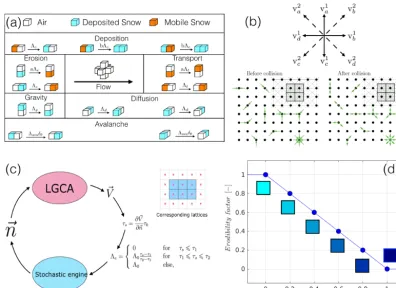
Figure 1.Description of the modelling framework.(a)Transition rules for CA of snow transport.(b)LGCA approach for simulating air flow. (c)Schematic of the coupling between the CA and the LGCA models.(d)A simple sintering mechanism that reduces snow mobilization as a function of its age. Note that(a)and(b)are adapted from Narteau et al. (2009).
these cells in this study has dimensions ofl0in the horizontal
direction and h0 in the vertical direction. The ratio of the
horizontal and vertical length scales is a model parameter and in our case, l0/h0=5. This allows for greater vertical
resolution in the model and is required for simulating snow bedforms that are typically much flatter and shallower than sand bedforms (Filhol and Sturm, 2015). Note that this ra-tio is a free parameter in the model and was chosen as such to have a balance between increased computational expense (due to increased number of cells in the vertical) versus better resolution of the snow surface. In any case, test simulations performed with even higher vertical resolution (not shown) did not modify the results much.
The model proceeds in the form of transitions of the cell states based on certain rules. In the ReSCAL model, these rules are based on nearest-neighbour cell pairings known as doublets. A list of phenomenologically important dou-blet combinations is made a priori. Each of these doudou-blet combinations can transition to a different doublet combina-tion. These doublet groupings are presented in Fig. 1a, where they are grouped into six different phenomenological mech-anisms, namely deposition, erosion, transport, gravity, diffu-sion and avalanching. Before we elaborate further, it would be beneficial to avoid connecting the above-listed mecha-nisms directly to physical processes with the same names
to avoid confusion. For example, erosion in the CA model is not directly linked to the different grain-scale entrainment mechanisms discussed in Sect. 1 even though at bulk scale, it is intended to produce the same effect.
type to be performed, the doublet to be transitioned as well as the value of the time step itself are stochastically chosen based on the value of the transition rates and the global state of the cells. A list of transition rates for the CA model used throughout this study is given in Table 1.
It is clear, therefore, that only the relative values of the transition rates are important. These rates are chosen to roughly reflect observations in reality. For example, at bulk scale, transport is far more rapid than erosion or deposition. Erosion itself is typically faster but a more local process com-pared to deposition, which is slower but occurs over larger length scales (consider a scenario of deposition of effluents from a plume). The processes of gravity and cross-stream diffusion (due to turbulence) are the fastest and slowest re-spectively. Avalanching is implemented in an extremely sim-ple manner following Bak et al. (1988) – if the local slope is larger than a critical angle, a cell at that location is moved to a random location down the slope. We realized a posteriori that for the scale of the dunes simulated in this study, avalanch-ing is of negligible importance, and thus it is not discussed further.
2.2 Description of the LGCA model for flow over snow surfaces
The flow overlying the evolving surface is simulated using the lattice-gas cellular automata (LGCA) approach. In this numerical technique, the fluid is modelled as a set of parti-cles lying on the nodes of a square (or cubical) mesh that is called alattice. A particle must lie on one of the nodes of the lattice at all times and each node of the lattice can hold only one particle at any given time. Furthermore, a particle can move only to the nearest or next-nearest neighbours in one time step of the simulation. In other words, the velocities that a particle may have are extremely limited, in both mag-nitude and direction. This is illustrated in Fig. 1b. The top panel in this figure shows for example, that a particle may move only to nearest or next-nearest lattice points. Thus, a particle may move in one of eight different directions and have two possible speeds. A time step in the LGCA consists of two sub-steps. The first is known as thepropagationstep, shown in the lower left panel, where all particles with non-zero velocities move to their destination lattice nodes. The incoming particles at each node are represented by the green arrows that all lead into lattice points. Note that different lat-tice points have different numbers of incoming particles. Af-ter this sub-step, it may happen that multiple particles (tem-porarily) lie on the same node. To impose the constraint that a node may have only one particle, N-body collision calcula-tions are performed between the incoming particles, and the particles obtain new velocities. These new velocities are rep-resented by outgoing green arrows from many lattice points in the lower-right panel of Fig. 1b. This step is known as the collision step. The lattice velocities as well as the N-body collision rules are adopted from D’Humières et al. (1986). As
boundary conditions for the fluid particles, the collision of a particle with a solid object or a wall is modelled as a sim-ple elastic collision (similar to the model of the ideal gas). The LGCA methodology further provides a simple way to convert lattice-based velocities to “real” velocity of the flow. Typically it is simply the average of the velocities of particles in a given neighbourhood.
The LGCA approach is in some sense a reduced-order model of the full Navier–Stokes equations achieved by im-posing strict constraints on directions and velocity values. Its development began with the pioneering work of Frisch et al. (1986) and was the precursor to more advanced lattice–Boltzmann methods. The LGCA model in ReSCAL is adopted from D’Humières et al. (1986). This modelling technique has the advantage that it is an extremely rapid method to simulate flow over complex surfaces, which is typically quite challenging for more traditional fluid sim-ulation techniques such as large-eddy simsim-ulations or even Reynolds’-averaged Navier–Stokes (RANS) models. In the context of its use in this study, the LGCA, by simulating flow over complex bedforms on the surface, provides values of the surface-shear stress at every location of the surface. The surface-shear stress is essentially computed as a gradient of the velocity (computed using LGCA) in the direction normal to the local surface. The surface (as well as the normal) is of course the result of the CA model for snow transport.
Of all the transition types, erosion is the only one directly linked to the morphology of the surface while all other transi-tions are independent of their location in 3-D space. This link between erosion and morphology is established by modify-ing the transition rate for erosion accordmodify-ing to location and making it a function of surface-shear stress, which due to surface morphology is heterogeneous. Thus, areas in the do-main with larger shear stress experience more erosion. In the ReSCAL model, the erosion rate is linearly dependent on ex-cess shear stress(τs−τ1)as
3e=30
τs−τ1
τ2−τ1
forτ1≤τs≤τ2, (1)
whereτsis the local surface-shear stress andτ1andτ2are the
lower and upper limits of the linear regime. Forτs< τ1, the
erosion rate is set to zero while forτs> τ2, the erosion rate is
at the maximum possible value of30. The values of30and
τ2−τ1are constant and act only as scale and slope parameters
respectively.τ1is equivalent to a threshold shear stress and
is kept as a free parameter. As is explained in Sect. 2.4, it is used to specify the wind speed. A subtle point to note is that the shear stress quantities are scaled with respect to the shear stress scale,τ0. This scale is not discussed or identified in
this study as it is not directly relevant to finding the kinematic scales of length and time.
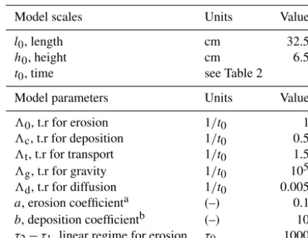
Table 1.CA model scales and parameters using in this study. See Fig. 1a for more information about the transitions and the doublets involved.
Model scales Units Value
l0, length cm 32.5
h0, height cm 6.5
t0, time see Table 2
Model parameters Units Value
30, t.r for erosion 1/t0 1
3c, t.r for deposition 1/t0 0.5
3t, t.r for transport 1/t0 1.5
3g, t.r for gravity 1/t0 105
3d, t.r for diffusion 1/t0 0.005
a, erosion coefficienta (–) 0.1 b, deposition coefficientb (–) 10 τ2−τ1, linear regime for erosion τ0 1000
aRatio of vertical to horizontal rates for both erosion and transport
mechanisms.bEnhancement factor for deposition due to DS-type cells.
undulating surface and the evolution of the surface itself is the defining feature of the ReSCAL model and thus makes it perhaps one of the best cellular automata models for simu-lating surface morphology that exists. This can be evidenced from the successful application of the ReSCAL model to simulate various complex sand bedforms on Earth (Zhang et al., 2010; Ping et al., 2014; Lü et al., 2017) and Mars (Zhang et al., 2012) and also gives us the confidence of in-troducing this model to the cryospheric science community. 2.3 Implementation of a simple sintering mechanism
for deposited snow
In this study, we intend to focus on the effect of sintering on snow bedform dynamics. For this purpose we implement a simple sintering mechanism that suits the CA modelling ap-proach. Every time a cell transitions to the “deposited snow” (DS) type, the time step of the simulation is noted. This pro-vides a way of measuring the age of the snow cell, i.e, the period of time a snow parcel rests in one place. All transition rates for transitions consisting of DS-type cells are then mul-tiplied by anerodibility factor,fE, which is simply chosen to
be a linearly decreasing function of the age of the cell with the most important transition being erosion. Thus, Eq. (1) de-scribing the erosion mechanism is modified as
3e=30fE
τs−τ1
τ2−τ1
forτ1≤τs≤τ2, (2)
with the erodibility factorfEbeing defined as
fE(t )= (
1−t−tdep
ts
fort−tdep≤ts
0 fort−tdep≥ts
, (3)
wheret is the current time of the simulation,tdepis the time
when the cell transitioned to a DS-type cell andtsis the
sin-tering timescale, i.e, the time after which a DS-type cell can-not perform any further transitions. This is a new parameter that must be chosen for such a model and we have chosen it to be 24 h. Thus, after 24 h, a DS-type cell will permanently remain in the same location for the rest of the simulation.
Cells that remain erodible, i.e., have ages less than 24 h are henceforth denoted as eDS-type cells while immobi-lized; sintered cells with ages greater than 24 h are denoted as neDS-type cells. This model is directly inspired by the approach of Filhol and Sturm (2015) and circumvents the requirement of accurate modelling of the highly complex and poorly understood phenomenon of sintering. The erodi-bility factor,fE, of snow cells as a function of their age,
t−tdep, is shown in Fig. 1d. The coloured boxes in Fig. 1d are
shown only to visually represent transition of eDS-type cells, coloured light blue, to neDS-type cells, which are coloured dark blue. A similar colour scheme is adopted in the follow-ing sections. Note that in the context of this study, erosion and erodibility refer only to the action of the wind. Erosion due to the impact of airborne snow grains on a moderately sintered snow bedform is not simulated and is kept for future work.
2.4 Finding the length and timescales of the CA model
A crucial contribution of Narteau et al. (2009), in addition to the development of the ReSCAL model, was the devel-opment of a methodology of translating results of CA mod-els, in which length (l0) and timescales (t0) are unknown, to
real units, thus allowing for intercomparison between simu-lations and data collected from field experiments. We present their approach and the related calculations of length and timescales used in this study below.
Consider a system consisting of air blowing over a flat granular bed. If the flow velocity is faster than a threshold velocity, the system is mechanically unstable, resulting in ae-olian transport and leading to the formation of the bedforms. For asmallperiod of time after aeolian transport commences, the system can be analysed using linear stability analysis, which identifies the fastest growing mode of the evolving sur-face. Past theoretical analyses (Hersen et al., 2002; Elbelrhiti et al., 2005; Claudin and Andreotti, 2006) have established this length scale,λmax, as being equal to 50ρsd/ρf, whereρs
is the density of the grains,ρfis the density of the overlying
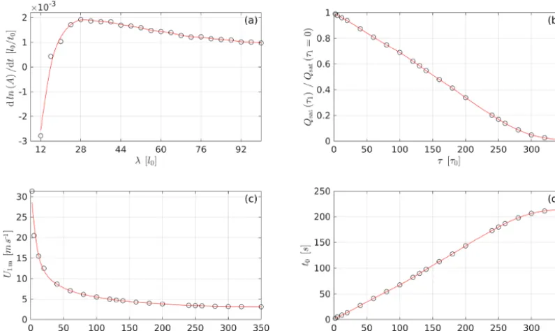
fluid (air in our case) anddis the mean grain size diameter. We performed a series of numerical experiments using the ReSCAL model where we simulate flow over a wavy surface with a different wavelength for each experiment and with an amplitude (A) of 2h0, which is the smallest amplitude we
λ=28l0. Thus,
λmax=28l0=50
ρs
ρf
d. (4)
Using values ofρf=1.00 kg m−3,ρs=910 kg m−3andd=
200 µm, we find the length scale of our model to be l0=
0.325 m.
Once the length scale has been identified, we can now pro-ceed to identify the timescale of the system. Returning to the system of air being blown over a flat surface, it has al-ready been established that a longtime after the initiation of the aeolian transport and with the wind speed being con-stant, the flux of grains in the air achieves a steady-state value known as the saturated flux Qsat. Past work, beginning
al-ready with Bagnold (1941) and refined over successive stud-ies using both field and wind tunnel data, has resulted in a semi-empirical formulation ofQsatas a function of material
and flow properties (Bagnold, 1936; Iversen and Rasmussen, 1999; Ungar and Haff, 1987). In effect, the saturated flux can be computed as
Qsat=25 s d g ρ f ρs
u2∗−u2c
, (5a)
with
uc=0.1 s
ρsgd
ρf
, (5b)
whereu∗ anduc are the friction velocity and the threshold
friction velocity for aeolian transport respectively.
If we consider an idealized scenario where the threshold velocity is zero with the resultant saturated flux value being Q0sat, a relationship relating saturated fluxes only as a func-tion ofu∗anduccan be found as
Qratiosat =Qsat Q0sat
=1−u
2 c
u2
∗
. (6)
This relationship is quite useful for CA-based modelling as the free parameter of τ1is essentially equivalent tou2c and
for modelling purposes can be chosen to be equal to zero. Thus, for different values ofτ1, the CA model provides the
left-hand side (LHS) of Eq. (6). We performed a series of experiments beginning with the idealized scenario of setting τ1=0 and gradually increasing the value ofτ1for each
in-dividual experiment. In each experiment we allowed the sys-tem to reach steady state and calculated the steady-state flux of snow in the air. The resulting values ofQratiosat as a function ofτ1are shown in Fig. 2b. OnceQratiosat ratios for different
val-ues ofτ1are found, we can compute theu∗in real units for a given value ofτ1. Note thatucis computed using Eq. (5b).
Using the log law, a givenu∗value can be converted to wind speed above a chosen height over the surface. Using a rough-ness length of z0=10−4m, wind speed at a height of 1 m
above the surface, denoted asU1 m, is computed and shown in
Fig. 2c. Once theu∗value for eachτ1is found, we can
com-pute the real saturated flux using Eq. (5a) and equate it to the model saturated flux. ThusQmodelsat l0h0/t0=Qrealsat m
−2s−1.
As the length scalesl0andh0are known,t0can be found as
a function ofτ1. Values of the timescalet0for different
val-ues ofτ1are shown in Fig. 2d. Note that the stress scale,τ0,
is not identified explicitly due to the fact that in addition to length and timescales, it would require a mass scale as well. Furthermore, since it is important only in terms of ratios and is directly related to the wind speed, it is not of major impor-tance to the current study.
Having established the length and timescales of the CA model, we choose three particular values ofτ1that are
typ-ically used in this study. These areτ1∈ {5,20,60}and are
equivalent toU1 m∈ {20.5,12.5,7.0}m s−1and denoted
fur-ther as high-wind (UH), medium-wind (UM) and low-wind (UL) cases respectively. Values of different quantities in-volved in calculating the timescales for these threeτ1
val-ues are provided in Table 2 with the full dataset of computed values for all the values ofτ1 provided in Table S1 in the
Supplement.
3 Results I: dynamics of fully developed snow barchans
In the first set of results we consider the motion of a solitary barchan dune and the effect of sintering on its motion and morphology. All simulations in this section follow a com-mon setup. The initial condition consists of a conical pile of unsintered snow with a given height and diameter of the base. The wind speed is equal to zero and thus there is no transport initially. We then choose one of the three different wind speeds as noted in Table 2 and first begin with only the LGCA model that accelerates the flow to eventually reach a statistically steady state. The snow cells are held in place dur-ing this spin-up phase. Once the flow is in equilibrium with the imposed initial snow bedform, the CA model is activated and the motion of snow cells is allowed to proceed. Note that the wind speeds described in the table and in text always refer tomeanor large-scale wind speeds at the height of 1 m above the surface. The effect of sintering is activated only once the dune is in steady-state motion. The lateral boundary condi-tions are periodic for both the flow and the particles, with the particles’ cross-stream location chosen randomly. Simu-lations are denoted as Cα, whereαrepresents the height of
the initial cone pile inh0units. Relevant quantities for
spe-cific dune simulations are presented below while details for all the dunes simulated are presented in Table S2.
cone-Figure 2.Establishing the length and timescales of the CA model.(a)Identifying the more unstable wavelength (see Eq. 4).λmax=28l0.
(b)Variation in theQratiosat withτ1.(c)Variation in the velocity at 1 m above the surfaceU1 mas a function ofτ1.(d)Identifying the timescale
t0of the model for different values ofτ1
Table 2.Details of the chosen wind scenarios for further analyses along with calculation of different quantities leading up to finding the relevant timescales for each wind speed.
τ1 Qratiosat (model or real)a ub∗ U1 mc Qmodelsat Qrealsatd t0e
(τ0) (–) (m s−1) (m s−1) (l0h0/t0) (m2s−1) (s)
5 0.9775 0.89 20.55 2.22×10⁻² 9.643×10⁻⁵ 4.868 20 0.9394 0.54 12.49 2.14×10⁻² 3.431×10⁻⁵ 13.148 60 0.8096 0.31 7.05 1.84×10⁻² 9.42×10⁻⁶ 41.276 aComputed usingQsatτ1
Q0sat , whereQ
0
sat=2.273×10⁻²l0h0/t0.bUsing Eq. (6), whereuc=0.134m s−1, using Eq. (5b).
cThrough the log law,u=u∗
κ log
z
z0
, whereκis the von Kármán constant (=0.4) andz0is the roughness length(=10−4). dComputed using Eq. (5a) using material properties as described in the text.eBy equating model and real saturated flux.
pile experiments allow for creating realistic barchans with-out having to describe their genesis. Additionally, the size of cone provides some guidance as to the dimensions of the barchan ultimately formed and thus allows for creation of barchans with a range of dimensions. Secondly, the effect of sintering in reality would begin as soon as snow is deposited on the surface, most likely through snowfall. By activating the effect of sintering on barchans in steady motion, we in-tend to isolate the interplay between the inertia of a barchan (which is a function of barchan size and wind speed) and the effect of sintering, which essentially acts as a damper for dune movement.
3.1 Steady-state barchan motion
Under the influence of constantly blowing wind, a conical pile morphs into a barchan dune that starts to move down-stream. In Fig. 3a, we show the top and side views of the evolution of the conical pile (case C20, with a constant wind speed ofU1 m=20.5 m s−1), into a barchan dune. Note
that the time is scaled using the sintering timescale(ts)of
The length and width of the dune is initially the same as the diameter of the cone, in this case, approximately 15 m, while the height of the cone is initially 1.1 m. After approximately 3ts, the morphology of the barchan, particularly its height,
is approximately constant, and thus we consider that steady state has been achieved. At steady state, the L, W and H di-mensions of the C20 dune are respectively 26.4 m, 22.75 m and 0.59 m.
We additionally also show the evolution of the length of the longest streamwise section of the barchan. This quan-tity is termed as the maximum streamwise length or MSL of the bedform (Ls). It has been shown that this is the
slow-est moving part of a barchan and thus is representative of the speed of the dune (Zhang et al., 2014). At steady state, we find Lsto be equal to 12.18 m. The relevance of Ls will
be more apparent in the coming paragraphs. It is interest-ing to note that it takes approximately 3ts or 72 h for this
dune to reach steady state. This is quite a long time consider-ing that we have the wind blowconsider-ing constantly for this period atU1 m=20.5 m s−1. Thus morphodynamics of the barchans
are much slower than typical sintering timescales. This point is elaborated upon further in the rest of the paper.
In Fig. 3c, we show four different measures of thespeedof the dune. In the field, one would typically track the location of the crest of the dune as a function of time. Other measures are also possible, such as tracking the displacement of the horn or the tail of the dune. Locations of the crest, tail and the horn of the barchan are tracked and plotted as a function of time. We find that all the speed measures are quite noisy, with the horn-based measure being most noisy and thus one to be avoided. To find the speeds, we thus resort to finding the slope of the best-fit line, values of which are provided in the legend of Fig. 3c. The horn-based speed measure is found to be the fastest, whereas the crest-based measure is found to be the lowest. Admittedly, the differences are minor, es-pecially compared to the fluctuations itself. We use an addi-tional measure based on tracking the centre of mass (COM) of the dune. In the field, this measure may be obtained by as-suming constant snowpack density and a laser scanner. This measure may be preferred as a more physically based and unbiased measure of dune movement and thus in the rest of this study dune speed is meant to be the speed of the COM of a dune.
An example of the cone-based experiments presented in the previous paragraphs and shown in Fig. 3 is repeated for 16 different cone (and thus barchan) sizes and two addi-tional wind speeds, namely the medium-wind UM (U1 m=
12.5 m s−1) and low-wind UL(U
1 m=7.0 m s−1) scenarios.
In Fig. 4a, we show the variation in dune speed with dune length for four different dunes for the UH wind scenario. We show both the instantaneous dune speed (computed every 50t0 steps, represented by circular symbols) and the
time-averaged velocity trends. This is to contrast the large instan-taneous dune speed fluctuations with a comparatively con-strained time-averaged value of dune speed. As expected,
dune speed decreases with the length (and thus size) of the dune. In Fig. 4b we show the variation in the dune speed of the same dune for the three different wind scenarios. Similar to the previous figure, there are large fluctuations of dune speed while the time-averaged value is more constrained. While differences between UH and UM cases are not sig-nificantly different, the dune in the UL case is almost 20 % slower than that in the UH and the UM cases. It must be noted that the effect of wind speed is not as significant as the dune size. Increasing the wind speed by a factor of 3 between the UL and the UH cases does not seem to induce a proportional response from the dune speed.
Thus, we have shown that the dune speed is inversely proportional to its height and directly proportional to wind speed. This is in fact a well-known property of barchans first recognized by Bagnold (1941) and quantitatively explored using field data by Elbelrhiti et al. (2005) for sand and by Kobayashi and Ishida (1979) for snow and in CA-type nu-merical experiments by Zhang et al. (2014). All these studies roughly proposed that
c∗= c
Q=f (1/H ) , (7)
wherecis the dune speed,Qis the saturated snow flux,c∗ is the normalized dune speed,H is the height of the dune andf is a linear function. We explore this scaling for snow barchans in Fig. 5.
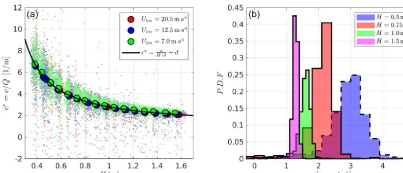
Long time averaging of both the height and velocity of the dune in each of the 48 simulations is carried out and the velocity-versus-height data points for all these simula-tions are shown in Fig. 5a. Simulasimula-tions are classified based on wind speed alone and coloured accordingly. Note that ve-locity is normalized by the flux of snow in each simulation. We find that all the simulation results, for different barchan dimensions as well as wind speeds, lie on a hyperbolic func-tion of H. The least-squares fit is found to be
c∗= c Q=
a
H+b+d , (8)
wherea,bandd are parameters with values of 1.7 (dimen-sionless),−0.1 m and 0.94 m−1respectively. In the same fig-ure, we also show the instantaneous values of normalized velocity as a function of height for each of the simulations. To further quantify the fluctuations in instantaneous veloc-ity, we show histograms of this quantity for four different barchans forU1 m=20.5 m s−1in Fig. 5b. We find that dune
speeds become more constrained with increasing dune size with the smallest (largest) dune having the most (least) broad histogram.
Figure 3.Morphodynamics of a solitary dune (case C20, high-wind scenarioU1 m=20.5 m s−1).(a)Visual representation of evolution from
a cone pile to a barchan. The final image is annotated for identifying different descriptors of a barchan.(b)Evolution of the length (L), width (W) and the maximum streamwise length (Ls) of the barchan.(c)Different versions of calculating the dune speed using the displacement of
the centre of mass (COM), tail, horns or crest of the dune.
Figure 4.Influence of(a)dune length and(b)wind speed on dune velocity. The instantaneous speeds are represented by symbols while the time-averaged speed is shown by thick lines. The wind speed in(a)is the UH scenario whereas the dune in(b)is the cone C24.
that such time averaging will be possible in the field, pri-marily due to fluctuations of mean wind speeds, effects of topography and the fact that the sintering process has sim-ilar timescales. On the other hand, due to large fluctuations of instantaneous velocity, a limited time series, even of a few hours, is unlikely to show any systematic trend. A possible solution could be to sample multiple mobile dunes, hopefully
of different sizes, at the same time using a laser scanner or photogrammetry.
Figure 5. (a)Dune speed normalized by snow flux(c/Q)as a function of height (H) for all the solitary dune simulations performed. Note that the instantaneous speeds are presented by small lightly coloured symbols. Time-averaged dune speeds for each simulation are shown by large symbols. Note that all symbols are coloured according to the wind speed of the simulation.(b)Probability distribution function of dune speeds for barchans of four different heights.
Doumani (1967), Kuznetsov (1960) and Kotlyakov (1961). It must be noted that these studies are quite old, and in future work we shall further compare our results with the latest dataset from Kochanski (2018) and Kochanski et al. (2018). Dune dimensions and speeds for all 48 simulations performed are provided for reference in Table S2.
3.2 Effect of sintering on barchan motion
We now turn our attention to understanding the effect of sin-tering on dune morphodynamics. In this section, we focus on the effect of sintering on barchans that are already in steady motion. This is achieved by “switching on” the effect of sin-tering only once the morphology and the mean dune speed has reached a steady state.
Sintering is activated in all 48 simulations with different barchan shapes and wind speeds. In general, three types of behaviours are observed. Firstly, the fastest-moving barchans continue their motion without much difference. On the other hand, the slowest-moving barchans seem to sinter “in place”; i.e, the barchan immediately ceases to move, without any sig-nificant change in morphology. The intermediate behaviour is found for a range of dune speeds in between the extreme cases where a small part of the dune is deposited as a non-erodible layer while the dune continues to move, albeit with slightly reduced dimensions on account of loss of mass due to sintering.
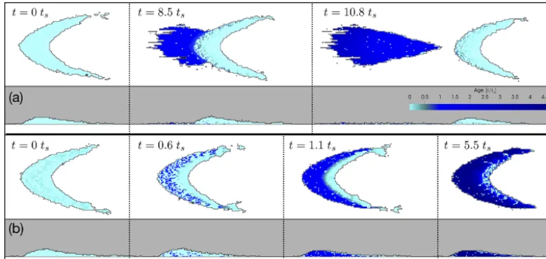
To illustrate these three different types of behaviours, we show in Fig. 6 the morphodynamics of the same barchan dune (C20: L, W, H, Ls=26.4, 22.75, 0.59 and 12.3 m) for
the UM and UL cases. The UH case is not shown because no perceptible difference in the morphodynamics is detected. For the UM case, shown in Fig. 6a, we find that the dune be-gins to leave behind a mass of snow that can no longer be
eroded. This mass originates at the tail end of the dune, which is the oldest part of the dune as we shall see further. The dune velocity is such that there is a continuous ejection of mass from the tail as the dune continues its downwind motion. Ul-timately, there is a split, where a sintered non-erodible mass of snow is left behind while a smaller barchan remains in-tact and mobile. In the UL case, the barchan sinters in place, and very quickly comes to a standstill. Notice that the shape and the dimensions of the barchan in this case do not change much once the sintering is activated. The morphodynamics of the two cases presented in Fig. 6 along with two additional cases are provided as Movies M1–M4 in the Supplement.
Figure 6.Effect of sintering on the morphodynamics of a mobile barchan (case C20):(a)medium-wind (U1 m=12.5 m s−1) and(b)
low-wind (U1 m=7.0 m s−1) scenarios. Note that the colour scheme is such that light blue colours represent mobile (eDS-type) cells while darker
shades of blue are sintered (neDS-type) cells.
The adjoining Fig. 7b quantifies the age distribution of the three panels in the form of cumulative distribution functions (CDFs) of ages with respect to wind speeds. For the UH case, we find that all of the barchan is younger than 0.3ts, and thus
sintering does not have a perceptible impact on its dynamics. On the other hand, for the UM case, even though most of the barchan is younger than the sintering timescale of 24 h, approximately 50 % of the barchan is older than 0.3ts. Thus,
there is an increasing influence of sintering on the dynamics of this barchan, evidenced previously in Fig. 6a. Finally, in the UL case, almost 50 % of the barchan has ages greater than the sintering time! Thus when the effect of sintering is activated, the barchan almost immediately ceases its motion and comes to a halt, thereby sintering in place.
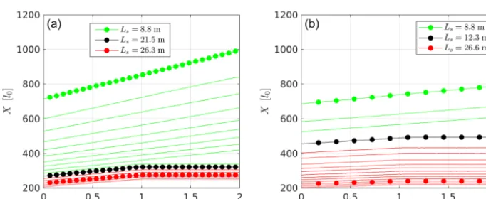
Recall that for each wind speed (UL,UM and UH), we per-formed simulations for 16 different barchans with increasing dimensions. These simulations allow us to identify the size of the barchan at which the effect of sintering is strongly felt. To do so, in Fig. 8a, we show the location of the tail of the different barchans once the sintering is activated for the UH case. The slope of each of these lines would correspond to the tail-based speed measure shown previously in Fig. 3c. With increasing size, the barchan speed decreases as previ-ously discussed. Lines are coloured green to indicate that the barchan speed does not change due to sintering. However, at a certain barchan size, there is a transition where, upon reaching sintering timets, the tail no longer moves; i.e, the
motion of barchan has been perturbed by sintering. We iden-tify that for the UH case, this occurs for barchan with MSL of Ls=21.5 m (line coloured black); all barchans with sizes
greater than this limit are also affected by sintering and show behaviour similar to that shown in Fig. 6b. A similar analy-sis for the UM case shows the limit to be at a barchan size
of Ls=12.3 m. In the UL case (not shown) all the chosen
barchan shapes sinter in place and thus the MSL is less than 8.8 m for this case.
These numerical experiments highlight the fact that the in-terplay between barchan dimensions, wind speed and the sin-tering rate impose a maximum length scale of any snow bed-form that can remain erodible and thus mobile. For example, in the UH case (U1 m=20.5 m s−1), the largest streamwise
dimension of any eDS-type bedform is limited to 21.5 m. Any bedform with dimensions greater than this limit (which perhaps arose earlier due to even higher wind speeds) will be strongly affected by sintering and will most likely sinter in place, thus converting to a neDS-type bedform. This limit decreases with wind speed and increases with the sintering rate.
In the following section, we move to a more realistic case where instead of beginning with a cone pile or even a barchan in steady motion, we directly simulate the effect of wind blowing over an initially flat fresh snow layer. As described earlier, the flat snow surface is mechanically unstable and rapidly evolves into various bedforms. Interestingly, we find that the results presented in this section remain valid there as well.
4 Results II: from transverse waves to barchans
In the previous section, results of numerical simulations of solitary barchans were presented along with the influence of sintering on barchans in steady motion. This helped us iden-tify the largest streamwise length scale that can exist in a mobile state with respect to wind speed and sintering rate.
simula-Figure 7.Distribution of age within a mobile barchan (case C24) prior to sintering.(a)Three panels show the distribution of age in the central slice as well as the arms of the barchan for the three different wind scenarios.(b)Cumulative distribution function of the age of the entire barchan for the three different wind scenarios.
Figure 8.Identification of the maximum streamwise length (MSL, Ls) for(a)high-wind and(b)medium-wind scenarios. In each figure,
the location of the tail of the barchan is plotted as a function of time. Lines from top to bottom represent barchans with increasing size. The lines are coloured to identify mobile (green) and immobilized (red) behaviours. The black line identifies the barchan at which this transition occurs.
tions where air is blowing over an initially flat snow-covered surface. This is a more realistic scenario that can be consid-ered to be equivalent to a scenario of strong winds after snow-fall. It is also more realistic in the sense that we do not im-pose any particular mobile bedform (such as a barchan in the previous section); bedforms such as merged barchans, trans-verse dunes, snow waves and sintered immobile snow de-posits emerge through self-organization of snow. Finally, we activate the effect of sintering from the first time step itself, once again reflecting our purpose to move towards simulat-ing more realistic scenarios.
Transition of a flat granular bed to an undulating sur-face with various bedforms under the action of overlying fluid flow has been investigated in the past, mainly in the context of the air–sand (aeolian) or water–sand (riverine) systems. Many such studies have in fact employed a CA-based framework similar to ours. There are two important mechanisms that these studies have revealed that are
Our hypothesis is that the sintering process, over time, causes the erodible snow deposits to convert to becoming non-erodible, thereby depleting snow supply and increasing the occurrence of barchans as opposed to an equivalent sys-tem without sintering. Additionally, it would be interesting to check whether the maximum streamwise length of a mobile snow bedform found in the previous section is indeed found in this more complicated system as well.
To confirm these hypotheses we perform simulations of flow over an initially flat snow layer of depth varying as 6.5 cm, 32.5 cm, 0.65 m or 1.3 m. These simulations are de-noted as H1, 5, 10 or 20 respectively, denoting the thickness in the CA height scaleh0. This set of four simulations was
performed for two different wind speeds, namely the UH and UM cases as in the previous section. The entire set of sim-ulations was repeated by deactivating sintering to provide a contrast and highlight the effect of sintering. Thus, in total 16 simulations were performed.
Each simulation has a domain size of 1000l0×1000l0×
100h0 in CA units or equivalently a domain of
approxi-mately 325 m in the horizontal directions and 6.5 m in the vertical. Care was taken to ensure that the vertical extent of the domain is adequate – additional simulations performed with larger heights showed no major differences. The hori-zontal boundary conditions in the lateral directions were pe-riodic.
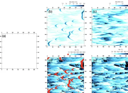
An illustration of the evolution of such a simulation (with sintering) and the information that can be extracted is pre-sented in Fig. 9. Top-view elevation of the surface in the UH-H20 case (i.e., U1 m=20.5 m s−1, initial snow depth
of 1.3 m) is presented at t=0ts (panel a) and att=50ts
(panel b). The initially flat surface is now reorganized into an undulating surface with multiple barchans, some laterally merged barchans and also some large-scale snow deposits that are sintered (neDS-type bedforms). The surface shown in Fig. 9b is filtered to remove all eDS-type cells revealing the underlying non-erodible snow layers in Fig. 9c. Such sintered deposits cover most of the surface area with the difference between the highest and lowest points of the sintered mass being approximately 40 cm. The age of the surface is pre-sented in Fig. 9d. The eDS-type cells are specially coloured red to highlight the fact that mobile bedforms are precisely the high-elevation regions in panel (b). Finally, in Fig. 9e, the mobile snow cells are filtered out to show the distribu-tion of age on the surface of the sintered mass. It is quite interesting to note the large distribution of ages with many clusters of old and new deposits in close proximity. Supple-ment Movies M5–M7 show the full evolution from the flat surface to undulating surface consisting of barchans and sin-tered snow deposits.
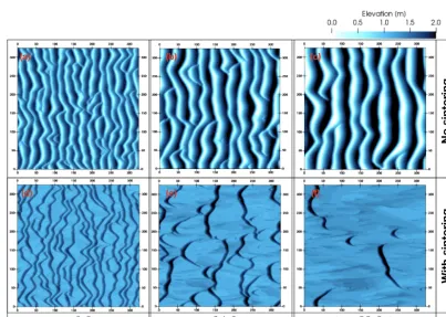
The following two figures provide some more insights into the effect of sintering on the snow bedforms. In Fig. 10, all six snapshots of the surface elevation maps come from the UH-H1 simulation with the shallowest snow layer with a depth of 6.5 cm. The upper panels (panels a–c) show results
from simulations without sintering while the simulation re-sults shown in the lower panels (panels e–f) account for the sintering effect. For comparison, the snapshots for the two simulations are presented at the three different times. In the left column panels (a, d), there is no major qualitative dif-ference between the simulations. Most bedforms have their dominant dimension in the cross-stream (transverse) direc-tion and are quite limited in their streamwise extent. Moving to the middle column (panels b–e), differences between the two simulations begin to emerge. In the non-sintering case (panel b), we find that the eDS-type cells are accumulated in a few bedforms consisting mainly of barchans and a long transverse dune. In comparison, in the with-sintering case (panel e), a few small barchans are found along with a few transverse dunes. There are also a few neDS-type cells form-ing large patches throughout the domain. Note also the fact that the dunes in panel (b) are higher than in panel (e). In the final right column, we find that in the non-sintering case, there are now a few barchans that have grown in size while the transverse dune is still present. In the corresponding with-sintering case (panel f), the neDS cell patches have grown in size and there are few eDS-type bedforms, consisting of a few short transverse dunes and small barchans. The differ-ence in the height between non-sintering and with-sintering simulations is even more clear in the rightmost column.
With a initial snow depth of 6.5 cm in the H1-type sim-ulations, there is a deficit in the sediment supply needed to form large transverse waves and the initial transverse waves break up into barchans. In the simulation without sintering, the individual barchans then grow in size. This was discussed at the beginning of this section and has been shown in previ-ous studies focussed on sand. Due to the additional sintering mechanism present in this study (and indeed in snow in real-ity), there is an additional curtailment of sediment available for aeolian transport and for forming bedforms. Thus the bed-forms in the case with sintering are smaller, flatter and more dispersed.
Figure 9.Evolution from an initially flat snow layer with a depth of 1.3 m to a complex dune field.(a)Initial condition of the simulation. (b)Elevation map of the surface att=50ts.(c)Elevation map of the sintered snow surface with the eDS-type cells filtered out.(d)Age of
the surface with eDS-type cells coloured in red.(e)Age of the surface with eDS-type cells filtered out.
the non-sintering case. As time progresses, more and more eDS-type cells are converted to neDS cells resulting in break-ing up of the transverse bedforms and patches of sintered snow, similar to the with-sintering case in Fig. 10. At a later stage (panel f), most of the earlier bedforms have disappeared completely, resulting in a few isolated barchans and short transverse dunes. In comparison to Fig. 11c, which shows large snow waves, the results in panel (f) are more similar to Fig. 10f instead (which it must be recalled had 20 times fewer snow sediment to begin with). Sintering indeed has a large impact on the bedforms that form on snow layers!
We concluded Sect. 3 by stating that the sintering mecha-nism imposes a maximum length scale (MSL) that a bedform can have to remain mobile. This length scale depends directly on wind speed and the sintering timescale. We restricted our analysis to a single sintering rate ofts of 24 h and only two
wind speeds – the UH (U1 m=20.5 m s−1) and UM cases
(U1 m=12.5 m s−1), which provided the maximum length
values of Ls=21.5 m and Ls=12.3 m respectively.
In Fig. 12, we present the maximum streamwise length of snow bedforms present in the domain as a function of time for all simulations UH-Hα (blue lines with symbols) and
UM-Hα(red lines with symbols), whereα∈ {1,5,10,20}. We additionally mark the limits suggested in the analysis in Sect. 3 for the UH (Ls=21.5 m, solid blue line) and the UM
(Ls=12.3 m, solid red line) cases. All simulations have a
maximum length scale that is ultimately below the limits sug-gested in Sect. 3. Thus the concept of sintering limiting the largest mobile snow bedforms, first developed from the soli-tary dune experiments, seems to be quantitatively applicable even in a more complex (as well as realistic) scenario of sur-face evolution from an initially flat sursur-face. Figure 12 pro-vides additional information. In particular, it is found that for all the UH-Hαcases, the MSL initially increases up to about 20ts, after which it begins to decrease and ultimately falls
be-low the MSL limit at approximately 140ts. For the UM case,
the initial increase in the MSL is found for only the H1 case, whereas for all the deeper snow layer simulations, the MSL decreases rapidly after 1tsalready. In the UM case it is also
interesting to note that the MSL values remain constant after approximately 120ts and that the largest MSL is found for
Figure 10.Evolution of an initially flat snow layer with a depth of 6.5 cm in the high-wind (UH) scenario.
Figure 12.Identification of MSL for the differentH αcases. Lines are coloured to represent the high-wind (UH, blue) and medium-wind (UM, red) scenarios. Corresponding values of MSL identified in Sect. 3 and in Fig. 8 are shown as thick solid lines for reference.
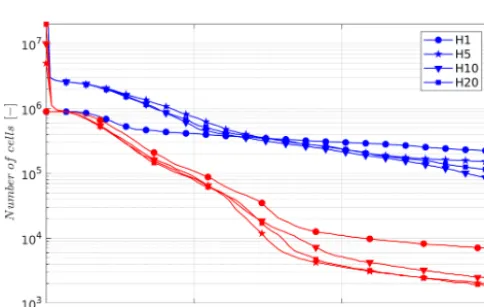
Figure 13.Total number of eDS-type cells left in the simulation as a function of time for differentH αcases. Lines are coloured to represent the high-wind (UH, blue) and medium-wind (UM, red) scenarios. Note that theyaxis is logarithmic.
In the final figure of our analysis, Fig. 13, the number of eDS-type cells in a simulation as a function of time is shown for each of the UH-Hαand UM-Hαcases. As the ini-tial condition for each of these simulations, recall that we consider a flat snow layer of differing depths. Each of these simulations begins with all the cells being of the eDS type, which, depending on their age, convert to neDS-type cells during the course of the simulation. Given that the horizon-tal dimensions of the domain in each of our simulations are 1000×1000, the number of eDS-type cells initially in a Hα-type simulation isα×106cells. The eDS-type cells essen-tially contain the only snow mass available for transport, the rest being sintered and permanently deposited. Firstly, the number of eDS cells decreases as a function of wind speed as shown by the curves of different colours, blue lines being for the UH case, while the UM cases are represented by red
lines. This implies that there is more permanent deposition as wind speed decreases – an admittedly intuitive result. For the same wind speed, comparing the results of snow layers of differing initial depths is rather counter-intuitive. The shal-lowest snow layer, H1 (i.e. depth of 6.5 cm) seems to have the largest number of eDS-type cells left in the latter stages of the simulation in the UH case and throughout the simulations in the UM case. This means that for medium to high wind speeds, shallow snow layers are more mechanically unstable and resist permanent deposition due to continual transport by wind. Furthermore, this difference between shallow and deep snow layers seems to increase with decreasing wind speed – at lower wind speeds, the shallow snow layers are compara-tively more unstable than deeper snow layers. This result is extremely important for polar regions, particularly Antarc-tica where precipitation amounts are small and wind speeds are high. The analysis presented here highlights the fact that fresh snow layers in Antarctica are mechanically highly un-stable.
5 Summary and outlook
In the first section in this study, we performed a series of nu-merical experiments to investigate the morphodynamics of a solitary barchan dune. A range of barchan sizes were simu-lated under the action of three different wind regimes repre-senting low-, medium- and high-wind scenarios. Even with-out accounting for the effect of sintering, some new insights were gained since the scale of dunes simulated (O 10 m), while relevant for snow bedforms, was an order of magni-tude smaller than barchans found in sand (O100 m), which are more well-studied. It was found that even small barchan dunes converge to Bagnold’s model for barchan speed as a function of their height. However, this convergence is achieved for very long time averages (between 18 and 36 h depending on the dune size). The instantaneous dune speeds have very large fluctuations and thus extracting any mean-ingful information from short time series of dune speeds is extremely challenging. While long time averaging is feasible in the framework of numerical experiments, it is highly un-likely that long time series of barchan speeds can be collected in the field. We also show that the variance of dune speeds decreases with barchan size. Finally, the effect of barchan size on dune speed is found to be far more prominent than the effect of wind speed. Overall, the motion of dunes of di-mensions ranging from (L, H)=(15.7 m, 0.4 m) to (60.5 m, 1.6 m) was simulated for three different wind speeds, namely U1 m=20.5, 12.5 and 7.0 m s−1. The fastest dune had a
ve-locity approaching 4 cm min−1(dune C14, UH case) while the slowest dune had a velocity of 0.12 cm min−1(dune C44, UL case). The values of the dune speeds were quite similar to those reported in literature.
three types of behaviour. Dunes smaller than a threshold size were found to continue their motion without any percepti-ble effect of sintering. On the other hand, dunes much larger than the threshold size were found to cease motion immedi-ately upon the activation of the sintering effect. For barchans with sizes close to the threshold size, it was found that a part of the dune becomes immobilized and permanently de-posited with the remainder of the dune maintaining its down-wind motion. The threshold size is determined in terms of the maximum streamwise length (MSL) of any snow bed-form (in this case a solitary dune). MSL is directly propor-tional to wind speed and to the sintering rate. We numer-ically found MSL to be equal to 21.5 m and 12.3 m for the high-wind (UH,U1 m=20.5 m s−1) and medium-wind (UM,
U1 m=12.5 m s−1) cases. For the low-wind cases, barchans
of all sizes were immediately sintered in place once sintering was activated and thus the MSL is less than 8.8 m.
In the following section (Sect. 4) we showed results of simulations of wind blowing over an initially flat surface of a snow layer of a finite depth. We considered snow layers with four different depths and two different wind speeds for our investigations (UH and the UM wind cases). The sin-tering process was activated from the beginning of the sim-ulation unlike simsim-ulations in Sect. 3. This scenario is more realistic and can be considered representative of the situa-tion of strong wind blowing after a relatively calm snowfall event. Each simulation was repeated by removing the sin-tering process, thus simulating a sand-like cohesionless ma-terial. This was done to clearly show the effect of sintering on snow bedforms. Qualitatively, we found that the initially flat and uniform snow layer reorganizes into a few mobile, erodible snow bedforms such as waves, transverse dunes and barchans. As time progresses, the dimensions of these bed-forms as well as their number decreases due to sintering. New, non-erodible snow deposits are found throughout the domain. These deposits are much shallower than the mobile bedforms while having larger dimensions in the horizontal direction. We find that the concept of sintering imposing a maximum streamwise length for any mobile bedform, first elucidated in Sect. 3, remains valid in this scenario as well. In spite of a large number of bedforms, each of which is chang-ing its dimensions as well as the speed while at the same time interacting with each other, we find that the MSL in the do-main is lower than or close to the limiting values found in Sect. 3 and described above.
Some additional valuable results are obtained as well. We find that whatever the depth of the fresh snow layer deposited may be, the amount of snow that remains erodible and thus available for snow transport remains the same in absolute numbers. We further find that shallow snow layers are more mechanically unstable compared to deeper snow layers and this effect is more pronounced for lower wind speeds. This result is particularly interesting for regions with small pre-cipitation amounts and moderate to strong winds. In such a
location, snow may never be permanently deposited and be continuously blown!
Cellular-automata-based modelling for snow bedforms has being introduced in this study with the intention of modelling the effect of sintering on snow bedforms and ultimately de-position. There are indeed various aspects of this study that need to be developed and advanced further to cover a full range of scenarios that would occur in reality. Firstly, a more physically based sintering model, suitable for the CA frame-work, should be adopted. A simple extension in future work could be to implement sintering rate as a function of mean air temperature and overburden pressure. Secondly, it would be important to implement a transition type in the CA model to account for erosion by snow-grain impacts on sintered sur-faces. This erosion mechanism is not currently taken into ac-count and thus prevents us from simulating erosional features such as sastrugi. Future works will focus on these develop-ments. Apart from these physical modelling improvements, numerical experiments could be performed over realistic to-pography underlying the snow layer, which would be espe-cially interesting for snowfall deposition in complex terrain. There are some caveats however to the CA-based mod-elling approach. The model parameters, consisting of differ-ent transition rates, are free parameters that have been ob-tained essentially by trial and error. Upon performing a sim-ulation, the time and length scales are established a posteri-ori by relating unstable modes and fluxes to those provided by theoretical formulations. We were fortunate to have been aided by previous studies using this approach in the sand community who compared it with field data in deserts. At a fundamental level, however, there is a need to constrain each of these parameters independently to physically based for-mulations. An attempt in this regard was made previously by Zhang et al. (2014), who used a simplified version of the ReSCAL model and derived relationships between the rate parameters and physical scaling laws. Such relationships could potentially be derived by using large-eddy simulations (LESs) of aeolian transport, the results of which can easily be translated into transition probabilities. Finally, even though in the present study we found barchan speeds to be fairly close to the few measurements that exist in the literature, new field campaigns, such as the recently published study by Kochanski et al. (2018, 2019), with a focus on surface morphology of snow surfaces, would be welcome for inter-comparison and verification.
regions where the underlying surface is exposed once again, whereas the erodible (and thus un-sintered) snow is localized in a few spots covering only a small portion of the overall sur-face area. How large would the differences in albedo of such surfaces be with and without accounting for wind-blown re-organization of snow?
The ultimate goal of CA-based modelling efforts would be to couple surface morphodynamics with regional-scale weather and climate models. CA-based modelling offers an extremely rapid yet robust methodology that couples aeolian transport of material and evolving surface morphology while being tightly coupled with atmospheric flow that co-evolves with the topography. An additional advantage is that it can be coupled to atmospheric models in an offline manner given the difference in timescales involved, further easing its adoption. As a future outlook, we feel that this methodology promises to be an exciting new tool in snow–atmosphere interaction study.
Data availability. All data described in this article are generated using the ReSCAL model, which is provided with the right to use and modify under the GPL license. The ReSCAL model can be found at http://rescal.geophysx.org/ (last access: 1 September 2018; ReSCAL, 2018).). The parameters and computational setup are de-scribed in detail in this article. Direct model outputs can be addi-tionally requested from the authors.
Supplement. The supplement related to this article is available on-line at: https://doi.org/10.5194/tc-13-3239-2019-supplement.
Author contributions. VS and ML formulated the research plan, VS developed the sintering algorithm, VS and LB implemented the al-gorithm and performed the simulations, VS carried out the analyses and developed the visualizations, VS, and LB and ML wrote the paper.
Competing interests. The authors declare that they have no conflict of interest.
Acknowledgements. We thank the authors of the ReSCAL model for providing it freely with the right to use and modify under the terms of GPL. We thank Etienne Vignon, Alexis Berne and Franziska Gerber for insightful discussions and Celine Labouesse for improving the quality of the paper. The group’s East Antarctica field campaigns are further supported by the National Institute of Polar Research, Japan and the Cryospheric Research Laboratory at Nagoya University, Japan (PI: Koichi Nishimura), and their help is gratefully acknowledged.
Financial support. This research has been supported by the “Lo-cal Surface Mass Balance in East Antarctica” (LOSUMEA grant)
project of the EPFL, the Swiss National Science Foundation (grant no. 160667), and the Swiss Supercomputing Center (CSCS) (grant no. s873).
Review statement. This paper was edited by Guillaume Chambon and reviewed by Clement Narteau and one anonymous referee.
References
Agosta, C., Amory, C., Kittel, C., Orsi, A., Favier, V., Gallée, H., van den Broeke, M. R., Lenaerts, J. T. M., van Wessem, J. M., van de Berg, W. J., and Fettweis, X.: Estimation of the Antarctic sur-face mass balance using the regional climate model MAR (1979– 2015) and identification of dominant processes, The Cryosphere, 13, 281–296, https://doi.org/10.5194/tc-13-281-2019, 2019. Amory, C., Trouvilliez, A., Gallée, H., Favier, V., Naaim-Bouvet,
F., Genthon, C., Agosta, C., Piard, L., and Bellot, H.: Compar-ison between observed and simulated aeolian snow mass fluxes in Adélie Land, East Antarctica, The Cryosphere, 9, 1373–1383, https://doi.org/10.5194/tc-9-1373-2015, 2015.
Amory, C., Naaim-Bouvet, F., Gallée, H., and Vignon, E.: Brief communication: Two well-marked cases of aerody-namic adjustment of sastrugi, The Cryosphere, 10, 743–750, https://doi.org/10.5194/tc-10-743-2016, 2016.
Amory, C., Gallée, H., Naaim-Bouvet, F., Favier, V., Vignon, E., Picard, G., Trouvilliez, A., Piard, L., Genthon, C., and Bel-lot, H.: Seasonal Variations in Drag Coefficient over a Sastrugi-Covered Snowfield in Coastal East Antarctica, Bound.-Lay. Me-teorol., 164, 107–133, https://doi.org/10.1007/s10546-017-0242-5, 2017.
Anderson, R.: A theoretical model for aeolian impact ripples, Sedimentology, 34, 943–956, https://doi.org/10.1111/j.1365-3091.1987.tb00814.x, 1987.
Anderson, R. and Haff, P.: Wind modification and bed response during saltation of sand in air, in: Aeolian Grain Transport 1, Springer, 21–51, 1991.
Anderson, R. S. and Haff, P. K.: Simulation of Eolian Saltation, Science, 241, 820–823, 1988.
Andreotti, B., Fourrière, A., Ould-Kaddour, F., Murray, B., and Claudin, P.: Giant aeolian dune size determined by the average depth of the atmospheric boundary layer, Nature, 457, 1120– 1123, https://doi.org/10.1038/nature07787, 2009.
Bagnold, R.: The movement of desert sand, Proc. R. Soc. London, Ser.-A, 157, 594–620, 1936.
Bagnold, R.: The Physics of Blown Sand and Desert Dunes, Springer Netherlands, https://doi.org/10.1007/978-94-009-5682-7, 1941.
Bak, P., Tang, C., and Wiesenfeld, K.: Self-organized criticality, Phys. Rev. A, 38, 364–374, https://doi.org/10.1103/PhysRevA.38.364, 1988.
Bartelt, P. and Lehning, M.: A physical SNOWPACK model for the Swiss avalanche warning Part I: Numerical model, Cold Reg. Sci. Technol., 35, 147–167, 2002.