www.atmos-meas-tech.net/5/2013/2012/ doi:10.5194/amt-5-2013-2012
© Author(s) 2012. CC Attribution 3.0 License.
Measurement
Techniques
Calibration of an all-sky camera for obtaining sky radiance at three
wavelengths
R. Rom´an1, M. Ant´on2,3, A. Cazorla2,3,*, A. de Miguel1, F. J. Olmo2,3, J. Bilbao1, and L. Alados-Arboledas2,3 1Laboratorio de Atm´osfera y Energ´ıa, Departamento de F´ısica Aplicada, Universidad de Valladolid, C/ Dr. Mergelina s/n,
47005 Valladolid, Spain
2Centro Andaluz de Medio Ambiente (CEAMA), Av. del Mediterr´aneo s/n, 18006 Granada, Spain
3Departamento de F´ısica Aplicada, Universidad de Granada, Campus de Fuentenueva s/n, 18071 Granada, Spain *now at: Department of Chemistry and Biochemistry, University of California, San Diego, 9500 Gilman Drive La Jolla,
California 92093, USA
Correspondence to: R. Rom´an (robertor@fa1.uva.es)
Received: 9 January 2012 – Published in Atmos. Meas. Tech. Discuss.: 23 February 2012 Revised: 25 July 2012 – Accepted: 25 July 2012 – Published: 21 August 2012
Abstract. This paper proposes a method to obtain spectral sky radiances, at three wavelengths (464, 534 and 626 nm), from hemispherical sky images. Images are registered with the All-Sky Imager installed at the Andalusian Center for Environmental Research (CEAMA) in Granada (Spain). The methodology followed in this work for the absolute calibra-tion in radiance of this instrument is based on the comparison of its output measurements with modelled sky radiances de-rived from the LibRadtran/UVSPEC radiative transfer code under cloud-free conditions. Previously, in order to check the goodness of the simulated radiances, these are compared with experimental values recorded by a CIMEL sunphotome-ter. In general, modelled radiances are in agreement with ex-perimental data, showing mean differences lower than 20 % except for the pixels located next to the Sun position that show larger errors.
The relationship between the output signal of the All-Sky Imager and the modelled sky radiances provides a calibra-tion matrix for each image. The variability of the matrix co-efficients is analyzed, showing no significant changes along a period of 5 months. Therefore, a unique calibration ma-trix per channel is obtained for all selected images (a total of 705 images per channel). Camera radiances are compared with CIMEL radiances, finding mean absolute differences between 2 % and 15 % except for pixels near to the Sun and high scattering angles. We apply these calibration matrices to three images in order to study the sky radiance distribu-tions for three different sky condidistribu-tions: cloudless, overcast
and partially cloudy. Horizon brightening under cloudless conditions has been observed together with the enhancement effect of individual clouds on sky radiance.
1 Introduction
Knowledge and measurements of the angular distribution of sky radiance (skylight at solar wavelengths, i.e. scattered sunlight) are important since the shape of human beings, ani-mals, plants, etc. is not regular or oriented to the Sun. There-fore, the sky radiance distribution has an outstanding role in the evaluation of radiation reaching complex targets like the human body or studies directed towards the development of solar energy systems.
plane perpendicular to the horizon that crosses the solar zenith angle, SZA, and zenith). Therefore, measurements of sky radiance are also useful to retrieve the aerosol optical properties.
Clouds produce the strongest changes in solar radiation with a substantial decrease of the direct component and an increase of the diffuse radiation, which lead to a decrease in global radiation (Alados et al., 2000; Alados-Arboledas et al., 2003; de Miguel et al., 2011b). The influence of the cloudi-ness on solar radiation has a significant spectral dependence, being weaker when the wavelength is shorter (Foyo-Moreno et al., 2001; Bilbao et al., 2011; de Miguel et al., 2011a). On the other hand, the clouds can also produce the enhancement of the solar radiation at surface, reaching levels even higher than its value at the top of atmosphere (Piacentini et al., 2010; Ant´on et al., 2011a). Therefore, studies about the behaviour of sky radiance and clouds are important for a better under-standing of cloud-radiation interaction.
Several authors have analyzed the sky radiance under dif-ferent sky conditions using several types of instruments. For instance, Grant and Heisler (1997), Grant et al. (1997a) and Grant et al. (1997b) used silicon photodiodes with filters, mounted on a platform that provided for rotational and incli-national motion, to take broadband radiance measurements in the ultraviolet range under obscured overcast, translucent overcast, and clear skies. Their system took a complete mea-surement of sky distribution (a grid of 10◦zenith and 3◦ in azimuth) in 30 min. Vida et al. (1999) tested a cloudless ra-diance model using rara-diance measurements taken by a pyro-electric radiometer (modified to present a 5-degree effective half angle field of view), and they found the highest differ-ences between modelled and experimental radiances close to the Sun. Weihs et al. (2000) took spectral radiance mea-surements under different sky conditions using a spectrora-diometer connected to a tube of fore-optics (1◦field of view) mounted in a tracker programmed to cover a full sky radiance distribution (a grid of 10◦in zenith and azimuth) in 15 min. Wuttke and Seckmeyer (2006) recorded measurements of sky luminance and spectral radiance using a sky scanner that took 150 points, in 40 s, evenly distributed across the sky. Both works (Weihs et al., 2000; Wuttke and Seckmeyer, 2006) compared radiance measurements with radiative trans-fer models based on the discrete ordinate radiative transtrans-fer algorithm, DISORT (Stamnes et al., 2000), and the results in-dicated that circumsolar region shows the highest errors, and the input parameters would have to be known with greater accuracy (e.g. they do not use PF as input).
Sky cameras, or sky imagers, are devices that combine a digital camera with a fisheye lens, or a hemispherical mir-ror in some cases, that takes pictures of the full hemispheri-cal sky. These instruments present two main features: firstly, they have a very high angular resolution taking measure-ments with a full hemispherical field of view, and secondly, these measurements are acquired simultaneously which
im-plies no problems with changes in atmosphere between two consecutive measurements at different viewing angles.
Sky imagers have been used for different purposes in re-search. Thus, these instruments were usually utilized to ob-tain cloud cover using threshold values for the ratio between different wavelength channels (Long et al., 2006). Heinle et al. (2010) developed an algorithm to discern the kind of cloud, and Mannstein et al. (2010) used a sky imager to de-tect and study contrails and additional cirrus clouds caused by air traffic. Aerosol optical depth (AOD) and cloud cover were retrieved using the All-Sky Imager and neural networks by Cazorla et al. (2008a) and Cazorla et al. (2008b), retively. L´opez-Alvarez et al. (2008) derived sky radiance spec-tra from sky images using a linear pseudo-inverse method, and Olmo et al. (2008a) used these spectra, and an itera-tive method based on radiaitera-tive transfer, to obtain AOD at 550 nm. Other authors used a sky imager with filters to mea-sure the relative sky radiance polarization (Horv´ath et al., 2002; Kreuter et al., 2009). Some works were performed using sky imagers carefully calibrated in the laboratory to obtain spectral radiance values (Voss and Zibordi, 1989; Zi-bordi and Voss, 1989; Voss and Liu, 1997; Cazorla et al., 2009).
The main aim of this paper is the calibration of a sky im-ager to obtain sky radiance measurements at three different wavelengths at Granada (Spain) using a radiative transfer model. The great advantage of the sky camera with respect to other instruments is its high time and spatial resolution. Additionally, the calibration method proposed in this work is simpler and cheaper than the methodologies found in litera-ture which need laboratory calibration.
This paper is structured as follows: Sect. 2 shows the loca-tion, instrumentation and the data used in the work. Section 3 describes the methodology used to obtain cloudless sky radi-ance values, and these estimated values are validated using radiance measurements. The full method for obtaining sky radiance from sky images is presented in Sect. 4. Results and conclusions are in Sect. 5, where the obtained calibration ma-trices are tested with measurements and a qualitative analysis of three sky images is presented. Finally, the conclusions are summarized in Sect. 6.
2 Site, instrumentation and data
2.1 Site
2.2 Instrumentation
2.2.1 The All-Sky Imager
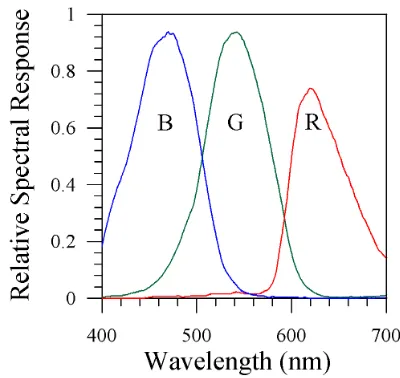
The All-Sky Imager designed and deployed by the GFAT has been operating at our experimental site since 2005 and basi-cally consists of a digital colour CCD camera with a fisheye lens encapsulated in an environmental housing that is tem-perature regulated with a peltier cell. The system is installed in a Sun tracker (2AP model from Kipp & Zonen) to block the direct solar radiation using a shadow ball. A transpar-ent acrylic dome protects the sky imager from the weather conditions like rain or snow. This dome was changed by a glass dome (non-acrylic) in December 2010 due to degrada-tion problems, being the new dome more stable. The camera body is a RETIGA 1300C (QImaging) and has a CCD sor with three channels: red, green and blue. The CCD sen-sor is the model ICX085AK from Sony working with a filter that blocks the wavelengths in the infrared region (standard configuration of the camera). The spectral responses of the camera channels are shown in Fig. 1, being centred around 450 nm, 550 nm and 650 nm with a bandwidth about 100 nm for the blue, green, and red channel, respectively. Spectral responses show a symmetrical shape except for the red chan-nel, because it is influenced by the infrared filter. The lens is a Fujinon FE185C057HA fisheye lens, its field of view being 185◦, which guarantees 180◦ field of view projected
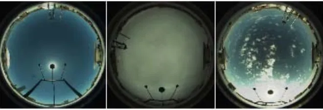
into CCD. The lens manufacturer indicates that there is no longitudinal or lateral chromatic aberration and the angular distortion is less than 0.8 %. The lens effect in the image was obtained using a ruler in a dome, observing that the variation of zenith angle is linear with the pixel distance (equidistant projection in the CCD), and the solid angle viewed by each pixel was calculated using this information (Cazorla, 2010). The final result of the camera is an image (900×900 pix-els) with 12-bits digitalization per channel. As an example, three recorded images can be seen in Fig. 2 for three differ-ent sky conditions: cloudless, obscured overcast and partially cloudy. There are notable differences between the three im-ages, showing the higher response in the blue channel when the sky is cloud-free, and brighter clouds when the sky is not overcast. The Sun tracker, blocking the direct radiation, and other obstacles surrounding the camera can be appreciated in the images.
The camera was programmed to take images every 5 min between sunrise and sunset with an exposure time of 12 ms. All information about the GFAT All-Sky Imager can be found in Cazorla (2010).
2.2.2 Sunphotometer CE-318
A sunphotometer CE-318 (CIMEL Electronic, France), which is the standard Sun/sky photometer used in the AERONET network (Holben et al., 1998), was installed next to the sky imager in the same rooftop. This instrument
(in-Fig. 1. Relative spectral response of the ICX085AK CCD sensor for the red (R), green (G) and blue (B) channels, taking into account the infrared filter included in the RETIGA 1300C camera.
cluded in the AERONET network) takes extinction measure-ments at 340, 380, 440, 500, 675, 870, 940 and 1020 nm us-ing filters, and they are used to retrieve aerosol properties such as AOD and Angstr¨om coefficients at different wave-lengths, except at 940 nm which is used to retrieve total col-umn water vapour colcol-umn.
In addition, measurements of sky radiance at 440, 500, 675, 870 and 1020 nm are registered by the sunphotome-ter using a sky collimator at high gain at different angles in the principal plane and the almucantar (the circle parallel to the horizon with the zenith angle equal to the solar zenith angle, SZA) configurations. These measurements are use-ful to retrieval aerosol optical and microphysics properties like columnar aerosol size distribution, complex refractive index, PF and SSA at different wavelengths following the AERONET procedures (Holben et al., 1998; Dubovik and King, 2000).
Calibration of this instrument was performed annually by AERONET-RIMA network. More details about CIMEL CE-318-4 can be found in Holben et al. (1998).
2.3 Data set
Different measurements were used in this work. From the measurements recorded by the All-Sky Imager, we only work with those recorded during the year 2011 in order to guaran-tee images with the glass dome.
Fig. 2. Sky images taken by the All-Sky Imager of GFAT for three different conditions: a cloudless sky (8 July 2011, 13:15 UTC) on the left, an obscured overcast sky (23 January 2011, 10:35 UTC) in the middle, and a partially cloudy sky (7 March 2011, 16:15 UTC) on the right.
α=
logAOD440
AOD675
log675440
, (1)
β=AOD500
0.5−α . (2)
In addition, the sunphotometer sky radiances measured with the 440 nm and 675 nm filters were provided by AERONET, but the products of the network are the radiances at the nomi-nal wavelengths of 441 nm and 677 nm due to the filter band-width. Radiance measurements using the 500 nm filter (nom-inal wavelength of 501 nm) are only available along two months in 2011, but they were used to test the calibration method in Sect. 5.1. Additionally, SSA values were also used in the work and, how they are retrieved using sky radiances, AERONET provides these values at the nominal wavelengths of 441 and 677 nm. The SSA values are only available at 441 and 677 nm, but we used the SSA at 550 nm, which was estimated as the mean between SSA441 and SSA677.
Similar method was followed for the PF values, which are only available at 441 and 677 nm (nominal wavelengths) in AERONET, and thus PF550 was estimated as the mean
be-tween PF441and PF677for each scattering angle. Finally,
wa-ter vapour column values, provided by AERONET, were es-timated using Sun direct measurements. All mentioned data provided by AERONET can be downloaded visiting the web-site http://aeronet.gsfc.nasa.gov.
The daily total ozone column, TOC, used in this work was measured by several satellite-based remote sensing in-struments: OMI collected in the Aura satellite (downloaded from http://disc.sci.gsfc.nasa.gov/giovanni) and GOME and GOME-2 data (supplied by the staff of the Remote Sensing Technology Institute, IMF, of the German Aerospace Cen-tre, DLR). These satellite data show, in general, an excel-lent agreement with reference ground-based measurements (Ant´on et al., 2009a, b).
3 Modelling cloudless sky radiance
The methodology used in this work for the absolute calibra-tion in radiance of the All-Sky Imager is based on the com-parison of its output measurements with the sky radiance val-ues estimated by the UVSPEC radiative transfer model under cloud-free conditions. This section presents the description of the inputs used in the code and the validation of the mod-elled radiance values against experimental data measured by the CIMEL sunphotometer.
3.1 UVSPEC model
The reference values of sky radiance were estimated by the LibRadtran software package (the 1.6 beta version was used in this paper), which main tool is the UVSPEC model, de-veloped by Mayer and Kylling (2005). The various radiative transfer equation solvers included in the UVSPEC have dif-ferent capabilities to calculate the radiative quantities in the Earth’s atmosphere. The radiative solver chosen to obtain sky radiance, on the Earth’s surface, was an improved version of the DISORT algorithm in C language (CDISORT) running in 18 stream mode. This solver was developed by Buras et al. (2011), and it uses the correction developed by Nakajima and Tanaka (1988) applying the directional distribution after secondary scattering of light in an atmosphere.
We run the UVSPEC model using the standard profiles and inputs indicated by Ant´on et al. (2011b) for the GFAT sta-tion at Granada. The standard atmosphere was mid-latitudes summer (from May to October) and winter (the rest of months). The extraterrestrial spectrum used was the pro-posed by Gueymard (2005). Surface albedo was considered as a fixed value of 0.2 for all wavelengths. Daily TOC was included in the inputs, and all simulations were run under cloud-free conditions.
are scaled in the chosen profiles. Legendre moments were used as phase function information input, and these moments were calculated using the PMOM tool, included in LibRad-tran package, which calculates the Legendre moments of a given phase function. The PMOM tool was run to obtain 200 moments with a scattering angle grid resolution for moderate forward peaks. The SSA and PF as inputs depended on the wavelength of the estimated radiance.
Finally, the UVSPEC outputs for each simulation were the radiances, in m W m−2nm−1sr−1, at a selected wavelength each 5◦and 1◦in azimuth and zenith angles, respectively. 3.2 Modelled vs. experimental radiance
Sky radiances measured by the CIMEL sunphotometer were used to study the reliability of the UVSPEC modelled radi-ances. For this goal, 50 almucantar cloudless measurements of radiance at 441 and 677 nm were chosen randomly. The cloudless radiances were calculated using UVSPEC and the inputs explained above, but changing the output angles for the almucantar angles and selecting the wavelengths of the sunphotometer. In addition, SSA441and PF441were used as
input for the calculations of radiance at 441 nm and SSA677
and PF677for the radiance at 677 nm.
The absolute value of the relative error, ARE, between modelled and experimental values was calculated, for each scattering angle, by the next equation:
χ (%)=100 %|RMOD−RMEAS| RMEAS
, (3)
whereχ is the ARE, andRMOD andRMEAS are the
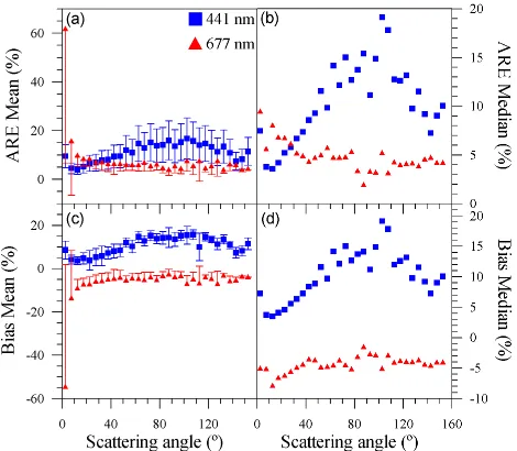
mod-elled (UVSPEC) and measured (CIMEL) sky radiances, re-spectively. ARE values were calculated for each scattering angle, which depends on the azimuth angle relative to the Sun’s azimuth and the SZA (Nakajima et al., 2006). Inter-vals of the scattering angle with a width of 5◦were taken us-ing the 50 random values (random solar zenith angles), and Fig. 3 shows the mean (panel a) and the median (panel b) of these intervals for the two wavelengths. The figure includes the standard deviation (error bars), which is only half repre-sented (up or down) for 677 nm due to the high value. The mean value of ARE for the sky radiance at 677 nm is about 60 % when the scattering angle is around 0◦. In contrast, the behaviour is remarkably good for angles far from the Sun. Thus, the mean parameter varies between 4 % and 10 % for scattering angles larger than 10◦and the standard deviation is
quite lower than near the Sun. Figure 3b shows that the me-dian values of ARE at 677 nm are smaller than 10 % for all scattering angles. This high difference between the median and mean of ARE at 677 nm for cases close to the Sun indi-cates that only a few modelled cases significantly differ with respect to the experimental data when the scattering angle is around 0◦. On the other hand, the mean and median values of ARE at 441 nm range are smaller for low scattering an-gles, and these values are lower than 20 % for all scattering
Fig. 3. Mean (left panels) and median (right panels) of the absolute relative error (ARE; upper panels) and bias (down panels) between sky radiance calculated by UVSPEC and measured by CIMEL for 441 and 677 nm as a function of the scattering angle in the almucan-tar. The error bars represent the standard deviation, of which only half (up or down) is included for 677 nm due to the high values near to the Sun.
angles. In addition, the mean and median of the bias (relative difference taking into account the sign) are shown in panels c and d. These values suggest systematic differences between the modelled values and the measurements with an underes-timation of the model for 677 nm and an overesunderes-timation for 441 nm.
Therefore, the sky radiance estimated with the UVSPEC model, and used in this work as reference for the calibra-tion of the All-Sky Imager, presents differences with respect to the experimental ones smaller than 20 % and 10 % for 441 nm and 677 nm, respectively. Nevertheless, we have de-cided to avoid the use of the UVSPEC simulations for those cases near to the Sun (azimuth angle relative to Sun smaller than 10◦).
4 Calibration method
code allows to simulate sky radiances at the same effective wavelengths of the camera channels. In addition, the use of experimental sky radiances is only useful for one pixel cali-bration but using a radiative transfer model all pixels can be calibrated.
4.1 Effective wavelength
In order to obtain the radiance reaching the All-Sky Imager at every pixel, it is necessary to simulate spectral radiance between 400 and 700 nm and weight them using the spec-tral response shown in Fig. 1 for each channel. This process expends a lot of computation time; moreover, we are inter-ested in obtaining spectral radiance instead of broadband. This issue is solved using the concept of effective wave-length (Kholopov, 1975). The ratio of two broadband mea-surements, taken with the same instrument, with its self spec-tral response, under different conditions, is also equal to the ratio of the same measurements but measured with an instru-ment that only is sensitive at the effective wavelength,λe.
Therefore, the effective wavelength for each channel is cal-culated using the following expression:
λe=
R
λ
λI (λ)S(λ)dλ
R
λ
I (λ)S(λ)dλ , (4)
whereλ is the wavelength,I is the irradiance reaching the instrument, and S is the spectral response of the channel (Fig. 1). In order to calculateλe, a different set of irradiances
reaching the camera is simulated using the UVSPEC model. A total of 200 simulations of spectral diffuse irradiance (di-rect irradiance does not reach the camera) were simulated per channel. The phase function used in these simulations is the Henyey-Greenstein function. In addition, the values of the asymmetry parameter and SSA are 0.7 and 0.9, respectively, and a fixed TOC value of 300 DU is utilized for all wave-lengths under a mid-latitudes summer atmosphere.
The 200 simulations for each channel (600 in total) were run changing SZA (from 10◦to 80◦in 10◦steps),α
parame-ter (from 0.2 to 1.8 in 0.4 steps) andβparameter (from 0.01 to 0.21 in 0.05 steps). Thus, 200 effective wavelengths per channel were calculated by Eq. (4) using the simulated spec-tral diffuse irradiances. The mean values were 464 nm (blue), 534 nm (green) and 626 nm (red), with a standard deviation of 2 nm for the three channels. Therefore, the spectral radi-ance reaching the camera is simulated at these three effective wavelengths as is described in Sect. 3.1, taking into account that the SSA and PF values used as inputs are SSA441 and
PF441to estimate the radiance at 464 nm, SSA550and PF550
for 534 nm, and SSA677and PF677for 626 nm. 4.2 Calibration matrix
First, a cloudless image is selected, being separated in the red, green and blue images. We mask the zenith angles higher
than 80◦, the pixels near to the Sun, and the different
obsta-cles around the whole sky like the shadow system and the two pyranometers installed on the tracking system near the camera (see Fig. 2). In the next step, the pixel counts were normalized to unity using the ratio between the raw value and the highest recorded value (216). Finally, the dark noise signal was removed taking into account that, in all rows and columns of an image, a dark zone appears whose signal must be null (as a first approximation). Therefore, the minimum values for each column and each row were averaged and con-sidered as the dark signal, which was subtracted to the nor-malized signal. Some authors (e.g. Voss and Zibordi, 1989; Voss and Liu, 1997) found problems related to the lens since its transmittance varies with the field of view. However, in this work, this issue was not considered because the cali-brated system consists of the CCD with the lens together, and the field of view of the lens presents no significant changes in the pixels between different images due to the angular sym-metry.
The corrected image is a 900×900 matrix, P, whichPij
el-ement is the corrected raw signal for theij-pixel. This signal should be proportional to the incident radiation: radiance that reaches theij-pixel multiplied by the solid angle of that view, ij. Therefore, a 900×900 matrix, R, was constructed using
the simulated radiance values (Sects. 3.1 and 4.1) and inter-polating for each pixel. Therefore, the matrix calibration, K, can be expressed as
K=R
P . (5)
This relationship is only valid if the response of the CCD sen-sor is lineal. The raw signal of the CCD, without removing the dark noise, was represented as a function of the simulated sky radiance for different cloudless images (not shown). The results indicate that the CCD response is linear for normal-ized raw values smaller than 0.8, being the pixel saturated for a signal higher than 0.8. Therefore, the pixels with normal-ized signal higher than 0.8 (before the subtraction of the dark noise) were removed along with their eight neighbours due to blooming effect (Voss and Liu, 1997).
From the method described here, given a cloudless im-age, three calibration matrices (RED, GREEN and K-BLUE) are calculated using Eq. (5). These matrices can be used to calculate the radiance at 464, 534 and 626 nm mul-tiplying the specific K matrix by the specific channel of the image and dividing this value by the solid angle viewed for each pixel.
4.3 Matrix calibration variability
A set of cloudless images were selected to study the variabil-ity of the matrix elements (Kij). The dates of the eight
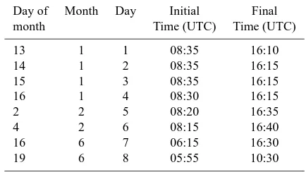
(day 1 to 4), and the variability in a long period (5 months) from winter days (day 1 to 6) to summer ones (day 7 and 8). Moreover, the eight selected days were completely cloud-free in order to see the intra-daily variation of the calibration matrix. Therefore, a K matrix can be obtained for each image recorded during the eight days shown in Table 1.
In order to analyze the influence of SZA on theKij
ele-ments, we evaluated the variability for eachij-pixel over a whole day. Thus, the intra-daily coefficient of variation,0, was calculated for eachij-pixel:
0ij=100 %
σ (Kij,T)
M(Kij,T)
, (6)
whereσ (Kij,T)andM(Kij,T)are the standard deviation and
the mean of the several values of Kij throughout the day.
Thus,0is a matrix whose elements indicate the daily varia-tion of eachKij.
Table 2 shows the percentage ofKijelements with0lower
than 10 % and the mean value of0 for each day. It can be seen that the intra-daily variation of the coefficients of the matrix calibration is small, with a mean value between 3.1 % and 5.4 % for all days and channels. In addition, the percent-age of coefficients with variations lower than 10 % is near to 100 % for all days. These results justify that we assume that K-RED, K-GREEN and K-BLUE do not depend on SZA, and that daily mean K matrix, Kd, obtained as the average of
all calculated K matrices in a day can be considered repre-sentative for that day. Thus, Kdis calculated for the eight
se-lected days, and the resulting matrices are compared to each other The matrix with the absolute difference between the Kd
of the m-day (Kd,m)and the n-day (Kd,n)is obtained as
1Kd,m,n(%)=100%
Kd,m−Kd,n
Kd,n
. (7)
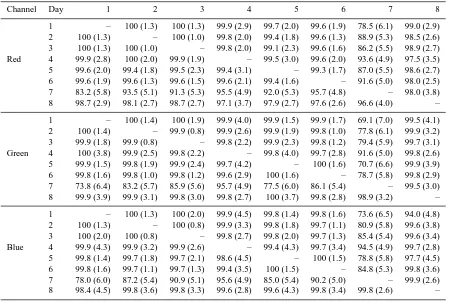
Table 3 reports about the inter-comparison between the eight days, showing the percentage of pixels with a difference lower than 10 % (1Kd,m,n<10 %) and the mean of these
differences in parentheses. The mean difference between the days 1, 2 and 3 is smaller than 2 % with 99.9 % of pixels with a difference lower than 10 %. This result indicates low variation in K between consecutive days. The highest mean difference between two winter days is 2.9 %, 4.0 % and 4.5 % for the red, green and blue channels, respectively. Moreover, the percentage of pixel with a difference lower than 10 % is always higher than 99 % when the winter days are compared for all channels. Table 3 also shows that the differences in-crease when day 7 is compared with the other days, being stronger in the green channel. This fact could be explained by some problematic images in day 7, because this day also shows the worst behaviour in Table 2. Nevertheless, the dif-ferences between day 7 and the others are smaller than 6.1 %, being within the margin of error given by the cloudless mod-elling. The highest value of1Kd,m,n(not shown in Table 3)
ranges from 14.8 % to 57.6 %, from 19.3 % to 152.5 %, and
Table 1. Image set, showing day, month, and time interval (images are every 5 min).
Day of Month Day Initial Final
month Time (UTC) Time (UTC)
13 1 1 08:35 16:10
14 1 2 08:35 16:15
15 1 3 08:35 16:15
16 1 4 08:30 16:15
2 2 5 08:20 16:35
4 2 6 08:15 16:40
16 6 7 06:15 16:30
19 6 8 05:55 10:30
Table 2. Percentage of elements of0lower than 10 %, for each day and channel. The mean value of0is given in parentheses.
Day Red Green Blue
1 97.1 (5.4) 99.1 (4.4) 100 (3.9)
2 99.1 (5.3) 99.4 (4.3) 99.3 (4.1)
3 99.9 (4.5) 100 (3.5) 100 (3.1)
4 99.8 (4.9) 99.9 (3.9) 99.9 (3.5)
5 100 (4.8) 100 (4.1) 100 (4.5)
6 99.0 (5.3) 100 (4.2) 99.9 (3.9)
7 98.0 (5.3) 99.2 (4.9) 96.0 (5.2)
8 99.6 (4.0) 100 (3.4) 100 (3.5)
from 16.8 % to 146.8 % for red, green and blue channels, re-spectively.
Once we have observed that the variability ofKijelements
is not significant, a unique calibration matrix for each chan-nel can be derived from all images recorded during the eight selected days (a total of 705 images per channel). Figure 4 shows three images with the calibration matrices and their standard deviation, both in m W m−2nm−1raw−1. The
ma-trices’ coefficients show uniformity for all angles in the three channels. The coefficient of variation is below 10 % in 99 % of the pixels, and its mean is lower than 6 % for all channels. However, a few pixels (less than 1 %) show large variabil-ity (white pixels for the standard deviation images in Fig. 4). This high deviation could be related to occasional little spots. Therefore, the three calibration matrices shown in Fig. 4 can be applied to the raw data measured by the All-Sky Im-ager and, thus, the sky radiance can be estimated at 464, 534 and 626 nm for all sky conditions.
5 Results and discussion
5.1 Validation of the calibration method
Table 3. Contingency table showing the percentage of elements of1Kd,m,nsmaller than 10 % as a function of days and channels. The mean
1Kd,m,nis given in the parentheses.
Channel Day 1 2 3 4 5 6 7 8
1 – 100 (1.3) 100 (1.3) 99.9 (2.9) 99.7 (2.0) 99.6 (1.9) 78.5 (6.1) 99.0 (2.9)
2 100 (1.3) – 100 (1.0) 99.8 (2.0) 99.4 (1.8) 99.6 (1.3) 88.9 (5.3) 98.5 (2.6)
3 100 (1.3) 100 (1.0) – 99.8 (2.0) 99.1 (2.3) 99.6 (1.6) 86.2 (5.5) 98.9 (2.7)
Red 4 99.9 (2.8) 100 (2.0) 99.9 (1.9) – 99.5 (3.0) 99.6 (2.0) 93.6 (4.9) 97.5 (3.5)
5 99.6 (2.0) 99.4 (1.8) 99.5 (2.3) 99.4 (3.1) – 99.3 (1.7) 87.0 (5.5) 98.6 (2.7)
6 99.6 (1.9) 99.6 (1.3) 99.6 (1.5) 99.6 (2.1) 99.4 (1.6) – 91.6 (5.0) 98.0 (2.5)
7 83.2 (5.8) 93.5 (5.1) 91.3 (5.3) 95.5 (4.9) 92.0 (5.3) 95.7 (4.8) – 98.0 (3.8)
8 98.7 (2.9) 98.1 (2.7) 98.7 (2.7) 97.1 (3.7) 97.9 (2.7) 97.6 (2.6) 96.6 (4.0) –
1 – 100 (1.4) 100 (1.9) 99.9 (4.0) 99.9 (1.5) 99.9 (1.7) 69.1 (7.0) 99.5 (4.1)
2 100 (1.4) – 99.9 (0.8) 99.9 (2.6) 99.9 (1.9) 99.8 (1.0) 77.8 (6.1) 99.9 (3.2)
3 99.9 (1.8) 99.9 (0.8) – 99.8 (2.2) 99.9 (2.3) 99.8 (1.2) 79.4 (5.9) 99.7 (3.1)
Green 4 100 (3.8) 99.9 (2.5) 99.8 (2.2) – 99.8 (4.0) 99.7 (2.8) 91.6 (5.0) 99.8 (2.6)
5 99.9 (1.5) 99.8 (1.9) 99.9 (2.4) 99.7 (4.2) – 100 (1.6) 70.7 (6.6) 99.9 (3.9)
6 99.8 (1.6) 99.8 (1.0) 99.8 (1.2) 99.6 (2.9) 100 (1.6) – 78.7 (5.8) 99.8 (2.9)
7 73.8 (6.4) 83.2 (5.7) 85.9 (5.6) 95.7 (4.9) 77.5 (6.0) 86.1 (5.4) – 99.5 (3.0)
8 99.9 (3.9) 99.9 (3.1) 99.8 (3.0) 99.8 (2.7) 100 (3.7) 99.8 (2.8) 98.9 (3.2) –
1 – 100 (1.3) 100 (2.0) 99.9 (4.5) 99.8 (1.4) 99.8 (1.6) 73.6 (6.5) 94.0 (4.8)
2 100 (1.3) – 100 (0.8) 99.9 (3.3) 99.8 (1.8) 99.7 (1.1) 80.9 (5.8) 99.6 (3.8)
3 100 (2.0) 100 (0.8) – 99.8 (2.7) 99.8 (2.0) 99.7 (1.3) 85.4 (5.4) 99.6 (3.4)
Blue 4 99.9 (4.3) 99.9 (3.2) 99.9 (2.6) – 99.4 (4.3) 99.7 (3.4) 94.5 (4.9) 99.7 (2.8)
5 99.8 (1.4) 99.7 (1.8) 99.7 (2.1) 98.6 (4.5) – 100 (1.5) 78.8 (5.8) 97.7 (4.5)
6 99.8 (1.6) 99.7 (1.1) 99.7 (1.3) 99.4 (3.5) 100 (1.5) – 84.8 (5.3) 99.8 (3.6)
7 78.0 (6.0) 87.2 (5.4) 90.9 (5.1) 95.6 (4.9) 85.0 (5.4) 90.2 (5.0) – 99.9 (2.6)
8 98.4 (4.5) 99.8 (3.6) 99.8 (3.3) 99.6 (2.8) 99.6 (4.3) 99.8 (3.4) 99.8 (2.6) –
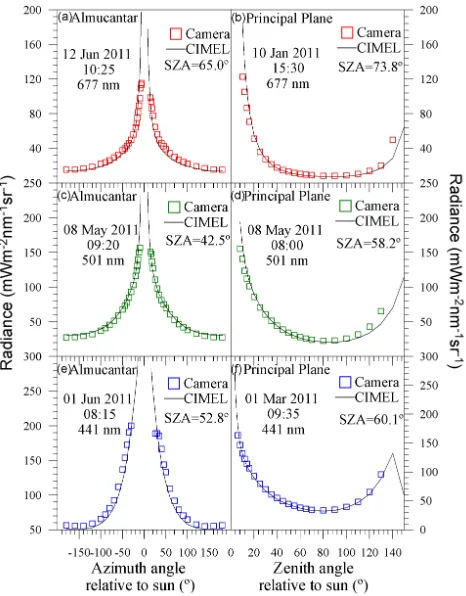
measured by the CIMEL sunphotometer. While this instru-ment measures the radiance at 441, 501 and 677 nm, the ef-fective wavelengths of the camera are 464, 534 and 626 nm. To solve these differences in the wavelengths of the channels, we obtain the ratios between the radiances at 677 nm and 626 nm (RatioR), 501 nm and 534 nm (RatioG), and 441 nm and 464 nm (RatioB) using the same 200 spectra of diffuse ir-radiance calculated in Sect. 4.1. The averages (±standard de-viation) of these ratios are 0.87 ± 0.07 (RatioR), 1.13 ± 0.06 (RatioG) and 0.98 ± 0.05 (RatioB). The camera radiance in a given solar direction was obtained as the average of the clos-est pixels in that direction (a square of 25 pixels). Thus, the multiplication of these radiances for the three averages ratios results in the estimation of the camera radiance at the CIMEL wavelengths.
Figure 5 shows the cloudless sky radiance measured by the sunphotometer and the estimations given by camera for the almucantar (left) and principal plane (right). Each panel corresponds to a particular case which was randomly selected with the unique condition that the time difference between the CIMEL and the camera measurements must be smaller than 10 min. It can be seen that CIMEL and camera radiances show a similar behaviour and sensitivity to scattering angle.
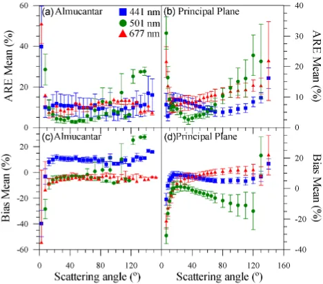
To evaluate the camera-CIMEL differences, the ARE mean values are calculated using 40 random cloudless
Fig. 4. Calibration matrices and their standard deviation (Std) in m W m−2nm−1raw−1, for the three channels.
The obtained errors in the camera radiances are higher than the sky radiances measured by CIMEL and used in in-version algorithms for aerosol properties. Therefore, the pro-posed method to obtain spectral radiance from a sky cam-era cannot be considered useful to estimate aerosol properties with inversion codes, but it can be useful for other applica-tions related to cloud properties or aerosol optical properties such as AOD,αandβ.
5.2 Application of the calibration matrices
Spectral sky radiances were calculated for three cases shown in Fig. 2, which correspond to three different sky conditions. Figure 7 (up) shows the sky radiance at 626, 534 and 464 nm (from left to right) under cloud-free conditions. It can be seen that the sky radiance decreases with wavelength in-creasing due to the strong spectral dependence of the molec-ular scattering. In addition, high radiance values are ob-served in the aureole along with a horizon brightening in the three wavelengths, in accordance with Wuttke and Seck-meyer (2006) who concluded that the reason for the horizon brightening can be explained by scattering processes in the atmosphere. The means (±standard deviation) of all pixel val-ues are 29 (±10), 53 (±17) and 88 (±24) m W m−2nm−1sr−1 for the 626, 534 and 464 nm wavelengths, respectively. The variation coefficient increases with the wavelength.
Fig. 5. The CIMEL and camera sky radiances together for two dif-ferent dates at 677 nm (a, b), 501 nm (c, d) and 441 nm (e, f). Left panels represent almucantar, and right panels are principal planes.
The radiance under obscured overcast conditions shows an opposite behaviour compared to under cloudless condi-tions. Thus, Fig. 7 (middle) shows that the radiances de-crease when the zenith angle inde-creases, which was related by Grant and Heisler (1997) in the visible and ultraviolet range. The highest radiances appear at 464 nm, and the ra-diance distribution looks more homogenous at 626 nm. In this case, the means (±standard deviation) are 71 (±14), 80 (±16) and 92 (±18) m W m−2nm−1sr−1for the 626, 534 and 464 nm wavelengths, respectively. The standard deviation is lower than in the cloudless sky, which is in accordance with the higher homogeneity of radiance distribution under over-cast. For these images, the variation coefficients are similar for the three wavelengths, around 20 %. Moreover, a high in-crease of radiance at 626 and 534 nm appears from cloudless to overcast conditions.
Fig. 6. Mean of the absolute relative error (ARE; a, b) and bias (c, d) between sky radiance retrieved by camera and measured by CIMEL for 677 nm, 501 nm, and 441 nm as a function of the scat-tering angle. Left panels represent almucantar, and right panels are principal planes. The error bars represent the standard deviation, of which only half (up or down) is included for 677 nm (almucantar) due to the high values near to the Sun.
the pixels. Therefore, individual clouds increase the diffuse radiation reaching the Earth’s surface. The coefficients of variation are higher under this condition than in the two be-fore and it increases with the wavelength, being the mean of the radiance (±standard deviation) using all pixels: 50 (±30), 60 (±30) and 90 (±40) m W m−2nm−1sr−1 for the
red, green and blue channel, respectively. The highest de-viation is caused by the differences between cloudless and cloud cover pixels. The blue channel shows a similar mean value in the cloudless and overcast conditions, which, due to its wavelength, is more affected by molecular scattering and, therefore, diffuse radiation is high also under cloudless con-ditions. However, clouds strongly increase the higher wave-lengths.
Finally, 120 images (40 for each condition) were selected and analyzed for each sky condition. The mean radiance per solid angle and its standard deviation were calculated for each image. The average of the mean radiance and its stan-dard deviation for the 40 cloudless images were 34 (±24), 55 (±29) and 89 (±40) m W m−2nm−1sr−1for the 626, 534 and
464 nm wavelengths, respectively, showing similar results as in the cloudless images of Fig. 7. In the case of overcast skies, the average radiances were 63 (±14), 70 (±16) and 80 (±18) m W m−2nm−1sr−1for the red, green and blue channel, re-spectively. Additionally, 73 (±35), 81 (±29) and 119 (±40) m W m−2nm−1sr−1were the average values of the radiance mean and standard deviation of the 40 partially cloudless im-ages for the 626, 534 and 464 nm wavelengths. These results
Fig. 7. Sky radiance (in m W m−2nm−1sr−1) at 626 nm (left), 534 nm (centre) and 464 nm (right) for top: a cloudless sky (8 July 2011, 13:15 UTC), middle: an obscured overcast sky (23 January 2011, 10:35 UTC), and bottom: a partially cloudy sky (7 March 2011, 16:15 UTC). Black regions represent the zenith angles higher than 80◦, the two pyranometers installed near the camera, and the saturated pixels. Figure 2 helps to discern saturated (white) and low-radiance (black) pixels.
are in agreement with all conclusions obtained from Fig. 7, where the coefficient of variation increases with the wave-length except for overcast skies when the coefficient of vari-ation is constant and close to 20 %.
6 Conclusions
Some important conclusions may be drawn from this work. The radiative transfer model UVSPEC estimates radiance values, under cloudless sky, similar to those recorded with a sunphotometer, obtaining the worst agreement between mod-elled and measured radiances near to the Sun. The mean dif-ferences between the modelled and measured sky radiances are lower than 20 % for all scattering angles when the median is considered. Thus, UVSPEC model can be used to estimate cloudless sky radiances if some inputs, such as aerosol scat-tering phase function, are taken into account.
scattering angles and close to the Sun, showing the radiance at 464 nm the lowest differences in these angles.
The radiance under overcast conditions presents the high-est homogeneity, while the larghigh-est variability in the radiance values corresponds to the partially cloudy conditions. Indi-vidual clouds increase the sky radiance at the higher wave-lengths, and the horizon brightening under cloudless condi-tions changes to horizon dimming when the sky is obscured overcast.
Finally, in future works, other analyses of sky radiances might be developed, e.g. the use of radiances for the retrieval of cloud properties, and a global study of sky radiances un-der different sky conditions. The retrieval of aerosol proper-ties using camera radiance information could be an option, but the radiance error given by the camera is too high for this purpose, and the camera wavelengths are not appropriated to obtain aerosol properties in the course mode. On the other hand, some aerosol optical properties such as AOD,α and β could be calculated from sky camera radiances. The au-thors encourage researchers and groups with available cam-era system to apply and use the proposed method to obtain sky radiance from sky images, because only radiative transfer modelling is needed to derive the calibration matrices.
Acknowledgements. The authors gratefully acknowledge the financial support extended by the Spanish Innovation and Science Ministry for the projects: CGL2011-25363 and CGL2010-12140E. Roberto Rom´an thanks Valladolid University for the support to research short stays and for the PIF-UVa grants for PhD students. This work was also partially supported by the Andalusian Regional Government through projects P08-RNM-3568 and P10-RNM-6299, the Spanish Ministry of Science and Technology through projects CGL2010-18782 and CSD2007-00067, and by the European Union through ACTRIS project (EU INFRA-2010-1.1.16-262254). The Remote Sensing Technology Institute (IMF) at the German Aerospace Centre (DLR) of GOME and GOME-2 instruments and the National Aeronautics and Space Administration (NASA) of OMI are also acknowledged for making available the ozone data required for this study.
Edited by: P. Stammes
References
Alados, I., Olmo, F. J., Foyo-Moreno, I., Alados-Arboledas, L. Es-timation of photosynthetically active radiation under cloudy con-ditions, Agr. Forest Meteorol., 102, 39–50, 2000.
Alados-Arboledas, L., Alados I., Foyo-Moreno I., Alc´antara A, and Olmo, F. J.: The influence of clouds on surface UV erythemal irradiance, Atmos. Res., 66, 273–290, 2003.
Ant´on, M., L´opez, M., Vilaplana, J. M., Kroon, M., McPeters, R., Ba˜n´on, M., and Serrano, A.: Validation of TOMS and OMI-DOAS total ozone column using five Brewer spectroradiome-ters at the Iberian peninsula, J. Geophys. Res., 114, D14307, doi:10.1029/2009JD012003, 2009a.
Ant´on, M., Loyola, D., L´opez, M., Vilaplana, J. M., Ba˜n´on, M., Zimmer, W., and Serrano, A.: Comparison of GOME-2/MetOp total ozone data with Brewer spectroradiometer data over the Iberian Peninsula, Ann. Geophys., 27, 1377–1386, doi:10.5194/angeo-27-1377-2009, 2009b.
Ant´on, M., Gil, J. E., Cazorla, A., Fern´andez-G´alvez, J., Foyo-Moreno, I., Olmo, F. J., and Alados-Arboledas, L.: Short-term variability of experimental ultraviolet and total solar irradi-ance in Southeastern Spain, Atmos. Environ., 45, 4815–4821, doi:10.1016/j.atmosenv.2011.06.020, 2011a.
Ant´on, M., Gil, J. E., Cazorla, A., Fern´andez-G´alvez, J., Vilaplana, J. M., Olmo, F. J., and Alados-Arboledas, L.: Influence of the cal-ibration on experimental UV index at a midlatitude site, Granada (Spain), Atmos. Meas. Tech., 4, 499–507, doi:10.5194/amt-4-499-2011, 2011b.
Bilbao, J., Rom´an, R., de Miguel, A., and Mateos, D.: Long-term solar erythemal UV irradiance data reconstruction in Spain us-ing a semiempirical method, J. Geophys. Res., 116, D22211, doi:10.1029/2011JD015836, 2011.
Buras, R., Dowling, T., and Emde, C.: New secondary-scattering correction in DISORT with increased efficiency for for-ward scattering, J. Quant. Spectrosc. Ra., 112, 2028–2034, doi:10.1016/j.jqsrt.2011.03.019, 2011.
Cazorla, A.: Development of a sky imager for cloud classification and aerosol characterization, Ph.D. thesis, University of Granada, Spain, 2010.
Cazorla, A., Olmo, F. J. and Alados-Arboledas, L.: Using a Sky Imager for aerosol characterization, Atmos. Environ., 42, 2739– 2745, doi:10.1016/j.atmosenv.2007.06.016, 2008a.
Cazorla, A., Olmo, F. J., and Alados-Arboledas, L.: Development of a sky imager for cloud cover assessment, Opt. Soc. Am. A., 25, 29–39, 2008b.
Cazorla, A., Shields, J. E., Karr, M. E., Olmo, F. J., Burden, A., and Alados-Arboledas, L.: Technical Note: Determination of aerosol optical properties by a calibrated sky imager, Atmos. Chem. Phys., 9, 6417–6427, doi:10.5194/acp-9-6417-2009, 2009. De Miguel, A., Mateos, D., Bilbao, J., and Rom´an, R.: Sensitivity
analysis of ratio between ultraviolet and total shortwave solar ra-diation to cloudiness, ozone, aerosols and precipitable water, At-mos. Res., 102, 136–144, doi:10.1016/j.atmosres.2011.06.019, 2011a.
De Miguel, A., Rom´an, R., Bilbao, J., and Mateos, D.: Evolution of erythemal and total shortwave solar radiation in Valladolid, Spain: Effects of atmospheric factors, J. Atmos. Sol-Terr. Phy., 73, 578–586, 2011b.
Dubovik, O. and King, M. D.: A flexible inversion algorithm for re-trieval of aerosol optical properties from Sun and sky radiance measurements, J. Geophys. Res. Atmos., 105, 20673–20696, doi:10.1029/2000JD900282, 2000.
Dubovik, O., Sinyuk, A., Lapyonok, T., Holben, B. N., Mishchenko, M., Yang, P., Eck, T., Volten, H., Munoz, O., Veihelmann, B., Van Der Zande, W. J., Leon, J., Sorokin, M., and Slutsker, I: Application of spheroid models to account for aerosol particle nonsphericity in remote sensing of desert dust, J. Geophys. Res.-Atmos., 111, D11208, doi:10.1029/2005JD006619, 2006. Foyo-Moreno, I., Alados, I., Olmo, F. J., Vida, J., and
Grant, R. H. and Heisler, G. M.: Obscured overcast sky radiance distributions for ultraviolet and photosynthetically active radia-tion, J. Appl. Meteor., 36, 1336–1345, 1997.
Grant, R. H., Heisler, G. M., and Gao, W.: Clear sky radiance distri-butions in ultraviolet wavelength bands, Theor. Appl. Climatol., 56, 123–135, 1997a.
Grant, R. H., Heisler, G. M., and Gao, W.: Ultraviolet sky radiance distributions of translucent overcast skies, Theor. Appl. Clima-tol., 58, 129–139, 1997b.
Gueymard, C. A.: Interdisciplinary applications of a versatile spec-tral solar irradiance model: A review, Energy 30, 1551–1576, 2005.
Heinle, A., Macke, A., and Srivastav, A.: Automatic cloud classi-fication of whole sky images, Atmos. Meas. Tech., 3, 557–567, doi:10.5194/amt-3-557-2010, 2010.
Holben, B. N., Eck, T. F., Slutsker, I., Tanr´e, D., Buis, J. P., Set-zer, A., Vermote, E., Reagan, J. A., Kaufman, Y. J., Nakajima, T., Lavenu, F., Janlowiak, I., and Smirnov, A.: AERONET – A federated instrument network and data archive for aerosol char-acterization, Remote Sens. Environm., 66, 1–16, 1998.
Horv´ath, G., Barta, A., G´al, J., Suhai, B., and Haiman, O.: Ground-based full-sky imaging polarimetry of rapidly changing skies and its use for polarimetric cloud detection, Appl. Optics, 41, 543– 559, 2002.
Kholopov, G. K.: Calculation of the effective wavelength of a measuring system, J. Appl. Spectrosc., 23, 1146–1147, doi:10.1007/BF00611771, 1975.
Kreuter, A., Zangerl, M., Schwarzmann, M., and Blumthaler, M.: All-sky imaging: a simple, versatile system for atmospheric re-search, Appl. Optics, 48, 1091–1097, 2009.
Long, C. M., Sabburg, J. M., Calb´o, J., and Pag`es, D.: Retrieving Cloud Characteristics from Ground-Based Daytime Color All-Sky Images, J. Atmos. Ocean. Tech., 23, 633–652, 2006. L´opez- ´Alvarez, M., Hern´andez-Andr´es, J., Romero, J., Olmo, F.
J., Cazorla, A., and Alados-Arboledas, L.: Using a trichromatic CCD camera for spectral skylight estimation, Appl. Optics, 47, 31–38, 2008.
Lyamani, H., Olmo, F. J., and Alados-Arboledas, L.: Physical and optical properties of aerosols over an urban location in Spain: seasonal and diurnal variability, Atmos. Chem. Phys., 10, 239– 254, doi:10.5194/acp-10-239-2010, 2010.
Lyamani, H., Olmo, F. J., Foyo, I., and Alados-Arboledas, L.: Black carbon aerosols over an urban area in south-eastern Spain: Changes detected after the 2008 economic crisis, Atmos. Envi-ron., 45, 6423–6432, doi:10.1016/j.atmosenv.2011.07.063, 2011. Mannstein, H., Br¨omser, A., and Bugliaro, L.: Ground-based obser-vations for the validation of contrails and cirrus detection in satel-lite imagery, Atmos. Meas. Tech., 3, 655–669, doi:10.5194/amt-3-655-2010, 2010.
Mayer, B. and Kylling, A.: Technical note: The libRadtran soft-ware package for radiative transfer calculations – description and examples of use, Atmos. Chem. Phys., 5, 1855–1877, doi:10.5194/acp-5-1855-2005, 2005.
Nakajima, T. and Tanaka, M.: Algorithms for radiative intensity cal-culations in moderately thick atmospheres using a truncation ap-proximation, J. Quant. Spectrosc. Ra., 40, 51–69, 1988. Nakajima, T., Tonna, G., Rao, R., Boi, P., Kaufman, Y., and Holben,
B.: Use of sky brightness measurements from ground for remote sensing of particulate dispersion, Appl. Optics, 35, 2672–2686, 1996.
Olmo, F. J., Cazorla, A., Alados-Arboledas, L., L´opez- ´Alvarez, M., Hern´andez-Andr´es, J., and Romero, J.: Retrieval of the optical depth using an all-sky camera, Appl. Optics, 47, 182–189, 2008a. Olmo, F. J., Quirantes, A., Lara, V., Lyamani, H., and Alados-Arboledas, L.: Aerosol optical properties assessed by an inver-sion method using the solar principal plane for non-spherical par-ticles, J Quant. Spectrosc. Ra., 109, 1504–1516, 2008b. Piacentini, R. D., Salum, G. M., Fraidenraich, N., and Tiba, C.:
Ex-treme total solar irradiance due to cloud enhancement at sea level of the NE Atlantic coast of Brazil, Renewable Energy, 36, 409– 412, 2010.
Rossini, E. G. and Krenzinger, A.: Maps of sky relative
radiance and luminance distributions acquired with a
monochromatic CCD camera, Sol. Energy, 81, 1323–1332, doi:10.1016/j.solener.2007.06.013, 2007.
Shettle, E. P.: Models of aerosols, clouds and precipitation for atmospheric propagation studies, in AGARD Conference Pro-ceedings No. 454, Atmospheric propagation in the uv, visible, IR and mm-region and related system aspects, Advisory Group for Aerospace Research Development (AGARD), Brussels, Bel-gium, 1989.
Stamnes, K., Tsay, S.-C., Wiscombe, W., and Laszlo, I.: DISORT, a General-Purpose Fortran Program for Discrete-Ordinate-Method Radiative Transfer in Scattering and Emitting Layered Media: Documentation of Methodology, Tech. rep., Dept. of Physics and Engineering Physics, Stevens Institute of Technology, Hoboken, NJ 07030, 2000.
Vida, J., Foyo-Moreno, I., and Alados-Arboledas, L.: The European Community Cloudless Sky Radiance Model. An Evaluation by Means of the Skyscan’834 Data Set, Theor. Appl. Climatol., 63, 141–147, 1999.
Voss, K. J. and Liu, Y.: Polarized radiance distribution measure-ments of skylight. I. System description and characterization, Appl. Optics, 36, 6083–6094, 1997.
Voss, K. J. and Zibordi, G.: Radiometric and geometric calibration of a visible spectral electro-optic “fisheye” camera radiance dis-tribution system, J. Atmos. Ocean. Tech., 6, 652–662, 1989. Weihs, P., Webb, A. R., Hutchinson, S. J., and Middleton, G. W.:
Measurements of the diffuse UV sky radiance during broken cloud conditions, J. Geophys. Res., 105, 4937–4944, 2000. Wuttke, S. and Seckmeyer, G.: Spectral radiance and sky luminance
in Antarctica: a case study, Theor. Appl. Climatol., 85, 131–148, doi:10.1007/s00704-005-0188-2, 2006.