Productivity or the External Environment: Which is
More Important for Growth in Emerging Markets?
Dzmitry Kruk
A B S T R A C T
Objective: Assessing and comparing growth promoting effects associated with productivity determinants and external environment determinants in 34 emerging market economies.
Research Design & Methods: The study is based on growth regression research design. Two different modelling frameworks – panel OLS and Arellano-Bond GMM estimator – are exploited. The study operates with a unique dataset, covering 34 emerging market economies over 11 years (2007-2017). A traditional set of growth regressors is enriched by the measures of productivity determinants. A set of country-specific measures of the external environment stance are computed and exploited in the modelling frame-work. Moreover, for capturing numerous attributes of growth promoting effects, the study considers alternative measures of economic growth.
Findings: Both productivity and external environment determinants are meaningful for growth in emerging market. However, external environment determinants dom-inate in explaining short-term growth, while productivity determinants are more im-portant for long-run sustainable growth.
Implications & Recommendations: The importance of external conditions for emerg-ing markets should not lead us to incorrect belief that productivity fundamentals do not matter anymore. Changes in the external environment are more likely to generate relatively short-term growth rate fluctuations. Hence, a country aiming to secure sus-tainable growth should still first of all think about productivity fundamentals.
Contribution & Value Added: The study allows to explain recent signs of decoupling between productivity gains and output growth without challenging the foreground role of productivity for generating growth.
Article type: research article
Keywords: economic growth; TFP; external environment; emerging markets JEL codes: F43, F44, O47, P24, P27
Received: 30 August 2018 Revised: 15 April 2019 Accepted: 17 April 2019
Suggested citation:
INTRODUCTION
As we are close to enter the 4th decade of economic transition in Central and Eastern Europe (CEE), there is a resurged interest in studies about growth in emerging markets (EM). To a large extent, it stems from the contradictions and collisions between growth theory predictions and recent evidence from EM.
The role of productivity (total factor productivity, TFP) gains in EM’s growth tends to be the central challenge herewith. Growth theory assumes that TFP gains must be the most powerful channel of growth. Before the Great Recession the majority of em-pirical studies on emerging markets mainly supported this vision (e.g. Klenow & Rodri-guez-Clare, 1997; Hall & Jones, 1999). This view became a kind of near-consensus, alt-hough some influential studies (e.g. Young, 1995) argued that capital accumulation was the most crucial for growth in EM.
The evidence from the current decade seems to be challenging that near-consensus on productivity. On the one hand, numerous studies document the deficit of TFP gains for the bulk of EM after the Great Recession (e.g. IMF, 2015, 2016, 2017; Adler et al., 2017). On the other hand, EM keep on growing and output growth definitely outpaces those of productivity (IMF, 2017). Hence, one may argue whether productivity is crucial for growth in EM any more.
Which growth determinant(s) can explain the mismatch between output and productivity growth and fill the gap in understanding the sources of growth in EM? A recent study by IMF (2017) puts external conditions as a key nominee for this role. It argues that just external conditions have contributed substantially to EM’s growth, compensating for the lack of productivity gains.
But this kind of response (if accepted) leads to numerous contradictions/challenges. For instance, whether the growth-enhancing effect of external conditions can be theoret-ically justified and treated as a persistent substitute to productivity. In practice, the latter means whether a current growth path in EM is sustainable. From the economic policy per-spective, it puts the issues of good growth-promoting policies again on the agenda. For instance, shall a country refocus from productivity enhancers to securing favourable ex-ternal conditions (e.g. through economic integration, trade agreements, etc.)?
Documented empirical evidence about the importance of external conditions for EM (e.g. IMF, 2017), is still not the ultimate diagnosis. Studies focused on detecting growth determinants are very sensitive to exploited data and methodology (Acemoglu, 2009; Cal-deron, Loyaza, & Shmidt-Hebbel, 2006). Hence, the issue of relative importance of exter-nal conditions and productivity requires more evidence and research.
GMM Arellano and Bond estimator – for estimating the growth effect of determinants of interest. Dual estimation framework provides robustness check, on the one hand, and se-cures enough room for economic interpretations, on the other hand.
The objective of the study is to assess and compare growth-promoting effects associated with productivity determinants and external environment determinants in 34 emerging mar-ket economies. Herewith, these two groups of determinants are treated as rivals in a sense.
The rest of the study is organised as follows. Section 2 provides a literature review and formulates the agenda for this study. Section 3 is devoted to data description and meth-odological issues. Section 4 reports and discusses the results. Section 5 concludes.
LITERATURE REVIEW
Since Solow (1957) a notion that TFP is the major channel of economic growth has become a cornerstone of the economic growth theory. The notion was reapproved within the endog-enous growth concept (e.g. Aghion & Howitt, 1992; Grossman & Helpman, 1991; Romer, 1990). However, empirical evidence on the patterns of economic growth is not that straight-forward. On the one hand, Hall and Jones (1999), Klenow and Rodriguez-Clare (1997), Wolff (1991) provide empirical support to the theory. On the other hand, Jorgenson, Ho and Stiroh (2005), as well as Christensen, Cummings and Jorgenson (1981) oppose it, stating that the mainstream approach underestimates the role of capital accumulation.
Empirical evidence on growth in EM supplies more food for reflection. Before the Great Recession, the mainstream approach admitted productivity and determinants behind it as the key for explaining growth in EM (e.g. Jones, 2016; Klenow & Rodriguez-Clare, 1997). But herewith the opposing empirical evidence was more convincing, especially at the level of individual countries. Young (1995), showed that the contribution of TFP to output growth in ‘Asian tigers’ was ‘not particularly low, …but not extraordinary high’. Torre and Colunga (2015) showed that in Mexico the contribution of TFP to growth between 1990 and 2011 was negative. Kruk and Bornukova (2014) argued that Belarusian growth was mainly due to capital accumulation. The estimates by De Gregorio (2018) showed that for numerous EM TFP gains between 1990 and 2014 were modest.
After the Great Recession the concerns about the role of productivity in EM’s growth intensified. Empirical evidence signals the lack of productivity gains in EM (IMF, 2015, 2016, 2017; Adler et al., 2017; Nezinsky & Fifekova, 2014). Apart from being crucially important itself, this challenge gives a rise to at least two additional concerns in respect to EM.
First, it resurges interest in the role of growth channels1 in terms of the growth
account-ing procedure. In other words, if acceptaccount-ing the statement of loweraccount-ing contribution from productivity, the point of interest is – which channel(s) has/have substituted the TFP one in securing growth in 2010s? For instance, IMF (2017) argue that decreasing TFP contribution during the last 15 years in EM was substituted by the ones associated with capital intensity
1 The sense of terms ‘growth channel (factor)’ and ‘growth determinant’ within this study confirms to the
(mainly) and human capital accumulation (to a lower extent). The latter, if accepted, casts doubts on the sustainability of this new growth regime, given theoretical considerations.
Second, the generally accepted view on growth determinants becomes questionable. The bulk of growth determinants highlighted in the literature may be systemised within three broad groups: institutions (Acemoglu, Johnson, & Robinson, 2001), technologies and ideas (e.g. Jones, 2016), and allocative efficiency (e.g. Hsieh & Klenow, 2009). The deter-minants within these groups are usually associated with productivity, i.e. they are treated to affect growth through the productivity channel. If there are doubts about the produc-tivity channel itself, these growth determinants should be re-examined as well.
Updating the debate about the role of external conditions in growth performance (e.g. Calderon et al., 2006; Arora & Vamvakidis, 2005), IMF (2017) argue that just external condi-tions are the growth determinant that have compensated for the lack of productivity gains. However, this kind of explanation does not offset all the contradictions mentioned above. First, if accepting external conditions as an alternative to productivity-based growth, we ac-tually must match corresponding determinants to other growth channels. Hence, shall we think about the external environment as the growth determinant acting through (physical or human) capital accumulation? Nevertheless, the rationale for treating external conditions as the growth determinant emphasizes its engagement just into the productivity channel of growth (Arora & Vamvakidis, 2005). Alternatively, shall we think about more sophisticated mechanisms of the impact of the external environment on productivity?
Second, presumably weakening growth and the strengthening role of external conditions are the phenomena that should be considered in different time dimensions. Treating external conditions as the determinant of long-term growth does not seem evident per se. Justification for linkages between the external environment and long-term growth mainly covers such in-stitutional features of external engagement as trade and financial openness (e.g. Dollar & Kraay, 2003; Edison, Klein, Ricci, & Slok, 2002). But as Calderon et al. (2006). show, even these linkages are not robust. In turn, matching such indicators of the external environment as the stance of external demand, trade conditions, financial conditions (e.g. IMF, 2017; Arora & Vamvakidis, 2005) to long-term growth outcomes might be even less theoretically justified. On the contrary, matching them to business cycle /short-term output fluctuations tends to be more natural (e.g. Paweta, 2018; Kaminsky, Reinhart, & Vegh, 2004).
Studying productivity and external conditions at the level of growth determinants (i.e. assessing and comparing their growth promoting effect) might be an important step to assemble the growth puzzle in EM in the last decade. According to Acemoglu (2009, p. 15), this approach serves as ‘the input into the types of theories that we would like to develop’. The approach is based on growth regressions pioneered by Barro (1991, 2001) as a tool for studying a conditional distribution of income among countries. However, it requires proper fine-tuning according to the pursued objective.
MATERIAL AND METHODS Methodology
, , = ∗ log ( , ) + β ∗ , + , (1)
where:
- output (per capita) growth rate;
, - level of output (per capita);
, β - coefficient and matrix of coefficients;
, - growth determinants;
, - error term.
However, three types of concerns are associated with this framework. First, nu-merous technical drawbacks may cast doubts on the results. Acemoglu (2009) summa-rises these drawbacks for the case of original specification and estimating through OLS as: (a) endogeneity; (b) room for misinterpretation of the economic sense of regression coefficients; (c) weak theoretical background of the approach for open economies. Hence, proper specification of growth regression and estimation technique are criti-cally important for the robustness of the results.
Second, a proper measure of growth on the left-hand side of the regression matters as well. Recalling the concerns about proper matching of external conditions to growth outcomes (either to business cycle or to long-term growth) makes the distinction be-tween output growth rates by time-horizon reasonable. Furthermore, for international comparisons a standard measure of growth (based on domestic SNA statistics) might also contain some drawbacks.
Third, the approach is extremely sensitive to the bundle of the growth determinants considered. Calderon et al. (2004) show that contradictions among researchers on growth determinants often occur because they operate with different sets of ‘nominees’ for growth determinants. For instance, Rodrick, Subramanian and Trebbi (2004) oppose the results of previous research arguing that ‘once institutions are controlled for … it ‘trumps’ everything else’. Hence, the initial set of growth determinants ‘nominees’ mat-ters and should reflect and correspond to the objectives of the exercise. Similar to this logic, incorporation of growth determinants closely linked with productivity into growth regressions with ‘standard’ determinants (including those associated with external con-ditions) might be an important step for puzzling out the collisions between productivity and external conditions in the context of growth in EM.
For mitigating technical drawbacks (b) and (c) of Barro-style growth regression (men-tioned above) the field has worked out an augmented approach that incorporates fixed effects model. Bearing this in mind, Acemoglu (2009, p. 85) argues that the following specification is meaningful for studying growth determinants:
log( , ) = ∗ log ( , ) + β ∗ , + + + , (2)
where:
, - level of output (per capita);
, β - coefficient and matrix of coefficients;
, - growth determinants; - country fixed effect; μ - time fixed effect;
, - error term.
In many empirical growth studies, to highlight the focus on growth rate (not level) this framework is modified through rearranging the first term from the right-hand side to the left-hand one and implicitly implying the restriction of = 1. Furthermore, for this study the focus on just two groups of growth determinants and treating them as ‘rivals’ is actu-alized through the absence of direct control for ‘standard’ growth determinants (e.g. initial conditions, integration into the global economy, etc.). However, allowing for a constant term, and both individual cross-section and time fixed effect is expected to capture the impact of such determinants. Finally, the following framework is employed:
, = + Α ∗ , + Β ∗ Ζ, + + + , (3)
where:
- output growth indicators; - common intercept Α, B - matrixes of coefficients
- the vector of external conditions indicators; Ζ - the vector of productivity indicators
- country-specific fixed effects - time fixed effect
- error term.
The specification (3) stems from theoretical considerations (Acemoglu, 2009, p. 85) and includes fixed effects (both in time and cross-section dimension) by definition. Hence, OLS fixed effects estimator is applied herewith (without prior econometric spec-ification tests, e.g. Durbin-Wu-Hausman test).
The specification (3) allows for a meaningful economic interpretation, but there might be doubts in robustness when estimating this specification. Arellano and Bond (1991) show that in cases when the panel is dynamic with rather small T and rather large N, the problem of endogeneity is likely to arise, leading to inconsistent estimates of the model. They worked out an alternative specification that solves the problem of endogeneity. In the application to this study Arellano-Bond estimator is specified according to (4). Follow-ing Arellano and Bond (1991), the specification (4) is estimated usFollow-ing generalised method of moments (GMM).
are differentiated by the time-horizon. The simplest choice for the response variable is an annual GDP per capita growth rate. However, this rate tends to be too volatile because of the contribution of the business cycle fluctuations. It is worthwhile to get rid of the latter, if bearing in mind the focus on the long-term growth. In other words, we should refocus on the trend2 of GDP and its growth rate. However, Coibion, Gorodnichenko, and Ulate
(2017) show that the vast majority of techniques aiming at getting rid of demand shocks fail to do so. Moreover, full refocusing on the trend growth rate might lead to ignoring that part of variation which could be assigned to demand shocks by mistake. So, we have a kind of a trap. The ‘raw’ measure of output growth is too volatile and includes unneces-sary fluctuations associated with demand shocks. At the same time, it is doubtful to obtain a credible measure of trend growth. In this situation, dealing with both time-horizons and treating corresponding output growth rates as alternative response variables might be a proper solution. Moreover, considering two time-horizons might be useful for detecting the properties of the alternative groups of growth determinants.
, = Γ ∗ , + Α ∗ , + Β ∗ Ζ, + + + , (4)
where:
, - output growth indicators; , - lagged dependent variable;
Α, Β, Γ - matrixes of coefficients;
, - the vector of external conditions indicators; Ζ, - the vector of productivity indicators;
- country-specific fixed effects; - time fixed effect;
, - error term.
Second, output growth rates are differentiated by the measurement concept. A ‘stand-ard’ one employs the growth rates of real GDP per capita for each country. However, these growth rates might keep too many common factors and ‘traces’ from the external environ-ment inside themselves. Hence, they might be excessively sensitive to external conditions. Employing relative indicators of countries’ well-being (with a common numeraire) and treating corresponding first differences as the measures of growth might eliminate/miti-gate ‘traces’ from external conditions. Hence, the study also employs the speed of closing the income gap (i.e. the ratio between the level of GDP per capita in a country vs. the one in the US3) of a country as the alternative measure of its output growth.
According to this concept, a country can ‘obtain some reward’ for more growth sus-tainability and less dependence on external shocks. For instance, if a country’s growth is more stable than the sample average one, but still close to the sample mean, the ‘stand-ard’ approach would not stress this country from the mass, while this approach would do this. Moreover, within ‘the speed of closing the income gap’ approach we can obtain a kind of a natural mechanism for the meaningful comparison of growth in countries with
2 The terms ‘potential output’ and ‘potential growth’ are frequently used in this context, as well. Following the
theoretical definition of ‘potential output’, it might reflect a ‘perfect’ way to remove demand shocks. But in practice, the term is frequently used in different meanings and I assume different techniques behind it. Hence, in order to avoid the misuse of the term and emphasize an ‘imperfect’ way of removing demand shocks, I use a more neutral term – trend output.
a substantially different level of well-being. At the same time, this measure by definition would display a strong correlation with the ‘standard’ growth rate4.
The values of all explanatory variables are standardised, which secures the compara-bility of explanatory power by different regressors in the model, basing on the estimated coefficients. Standardised values are computed according to:
=( ! "#)
$# (5)
where:
- standardized value of ; - explanatory variable i;
% - mean value of ;
&% - standard deviation of .
The process of estimation assumes a multi-step approach with sequential inclusion of explanatory variables, starting from external conditions indicators, while productivity indica-tors are included only after them. This procedure assumes to secure the external environ-ment indicators to ‘realize all their explanatory potential’ and allows tracking for the stability and significance level of the estimated coefficients, which serves as a kind of robustness check. If Ζ variables can add and/or ‘pull-over’ some explanatory effect from variables, it would witness the importance of productivity as straightforward growth-enhancers. If the procedure of saturating a model with explanatory variables exhibits robust results (stable and significant coefficients), an opposite exercise is done – sequential cut, i.e. getting rid of insignificant variables. The latter leads to the best specification of a model, which is reported in the article. If models with the same response variables based on the specifications (3) and (4) exhibit similar results, it witnesses robustness of the results. If that is the case, the speci-fication (3) may be used for the decomposition of growth by growth determinants.
The Sample and Sources of Data
For the objective of the study, the sample of 36 countries traced by EBRD (2017) is meaningful. Two countries – Kosovo and Uzbekistan – are excluded from the sample, because of the lack of data. So, the sample includes 34 countries: Albania, Armenia, Azerbaijan, Belarus, Bosnia and Herzegovina, Bulgaria, Croatia, Cyprus, Egypt, Estonia, Georgia, Greece, Hungary, Jordan, Kazakhstan, Kyrgyz Republic, Latvia, Lebanon, Lith-uania, Macedonia, Moldova, Mongolia, Montenegro, Morocco, Poland, Romania, Rus-sia, Serbia, Slovak Republic, Slovenia, Tajikistan, TuniRus-sia, Turkey, Ukraine. From this sample, Belarus and Tajikistan are considered only for growth measurement, but ex-cluded from modelling exercises, because of the absence of data on explanatory varia-bles. The main source of the data is the World Development Indicators (WDI) database of the World Bank.
The period sample is 2007-2017. It is justified for two reasons. First, productivity indicators based on the methodology by WEF (2017) have been available only since 2007. Second, just this period complies with the trend of an increasing role of the ex-ternal environment for EM (IMF, 2007).
4 For the sample of 34 countries considered, the coefficient of correlation between these two measures of
Response Variables
Combining both dimensions – time-horizon and the measurement concept – the study operates with four measures of output growth.
A ‘standard’ shorter-term growth rate is computed according to:
'(, =))!,*+,!,* (6)
where:
'(, - a ‘standard’ shorter-term output growth rate for a country i;
., - GDP per capita of country i (in Geary-Khamis 2011 international dollars). A ‘standard’ longer-term growth rate is computed according to:
'(_0(, = 1))!,*+2!,* 3
,
2 (7)
where:
'(_0(, - a ‘standard’ longer-term output growth rate for a country i;
., - GDP per capita of a country i (in Geary-Khamis 2011 international dollars). A shorter-term growth rate according to ‘income gap’ concept is computed according to:
4, = 56, − 56, (8)
where:
4, - a shorter-term output growth rate of a country i according to income gap concept;
56, - the ratio of GDP per capita (in Geary-Khamis 2011 international dollars) in
a country i to the one in the US.
A longer-term growth rate according to the ‘income gap’ concept is computed ac-cording to:
4_0(, =(89!,* 89:!,*+2) (9)
where:
4, - a shorter-term output growth rate for a country i according to income gap concept;
56, - the ratio of GDP per capita (in Geary-Khamis 2011 international dollars) in
a country i to the one in the US.
External Conditions Indicators External demand
The approach for computing country-specific external demand conditions is based on Arora and Vamvakidis (2005). First, the procedure assumes identifying the major trade partner for each country from the sample. The rule for forming the corresponding list assumes that the share of exports going to major trade partners should not be less than 70% of total exports for each year. Having formed the list, total exports to these coun-tries are assigned as ‘new total exports’ of the domestic country, and corresponding shares are recalculated basing on it.
partners), imports, GDP, etc. Two from these options are employed: total imports and GDP per capita growth rates. The latter leads to generating two alternative series of external demand. When estimating the models, the series with better explanatory power is included in each model.
Third, the indicator of external demand growth is computed according to:
;<_'(, = ∑ ∈A!>, ∗ '(_<;? , (10)
where:
;<_'(, - external demand growth for a country i;
B - trade partners of a country i;
>, - the share of a country j in a country i’s exports; '(_<;?, - indicator of demand growth in a country i.
If real imports growth rate is used for '(_<;?, external demand is noted as ;<_'(. In the case of real GDP per capita growth rate, the notation used is ;<2_'(.
Financial conditions indicator
Each country is assigned to a specific sub-region, for which financial conditions indica-tors are computed. The indicator for the corresponding sub-region represents a country in the modelling framework. Eleven sub-regions are considered: advanced EU, South-East EU, South-South-East non-EU, Central Europe, CIS, Caucuses and Central Asia Oil Import-ers, Caucuses and Central Asia Oil ExportImport-ers, MENA Oil ImportImport-ers, Asia Pacific, Russia and Turkey. Two large countries – Russia and Turkey – turn out to be too influential for the dynamics of financial flows for the whole region if including them according to the geographical and economic criterions. All other regions consist of a number of countries (the majority of which are not from those 34 considered in the study). For each sub-region the following indicator is computed:
4DE, = ∑ >∈ , (FG5, + H5, + I5, )/6GH, (11)
where:
4DE, - financial conditions indicator for a sub-region i; >, - the share of a country j GDP in i’s region GDP; FG5, - foreign direct investments inflow in a country j;
H5, - portfolio investments inflow in a country j; I5, - other investments inflow in a country j; 6GH, - GDP of a country j.
Trade conditions
Trade conditions indicator is computed for each country as the ratio between exports and imports prices according to:
0(D, =L_K%_K!,*!,* (12)
where:
0(D - trade conditions for a country i;
Productivity Indicators
Productivity determinants for the study are taken from the database by WEF (2017). WEF (2017) argue that it ‘…aims to measure factors that determine productivity, be-cause this has been found to be the main determinant of long-term growth’. Moreover, they provide some empirical evidence showing that the indicators have an explanatory power for growth (WEF, 2017, p. 4). They name an aggregate index as Global Competi-tiveness Index (CGI), but emphasize that understand competiCompeti-tiveness herewith ‘as the set of institutions, policies, and factors that determine the level of productivity of an economy’ (WEF, 2017, p. 11). CGI consists of 114 indicators grouped by 12 sub-indexes, which in turn form 3 broad groups (WEF, 2017).
The methodology of WEF (2017) assumes that in each year a country obtains a score between 1 and 7 on each indicator, which is the aggregation of corresponding numerous sub-scores on every indicator. However, the criterions on every sub-indicators may change somehow in time, reflecting changing global standards. From this perspective, a progress in any indicator is more a sign of improving country’s stance on relative basis (i.e. vs. the frontier economies), rather than on absolute one. For instance, if a country have improved its performance on a particular indicator, but the global (and especially corresponding frontier economies) progress has been more intensive, a score of the country is likely to deteriorate in comparison to previous period. The latter facilitates to the stationarity of the data on individual indicators from panel view (i.e. as a rule, there is no common unit root for a set of countries).
Given their economic sense and statistical properties, WEF sub-indexes are good productivity determinants ‘nominees’. However, 12 determinants of productivity as ex-planatory variables might be redundant, especially taking in mind (i) individual produc-tivity indicators are likely to be correlated with each other, thus causing to multicolline-arity; (ii) the lack of degrees of freedom, given that the sample is not so big. Hence, extracting principal components (5 ones for this study) from the whole set of WEF productivity sub-indexes is more reasonable.
Data Summary
Table 1 reports the list of the indicators used in the study, their notation and short description.
Specifications (3) and (4) assume that right-hand side variables are stationary. Hence, their stationarity is to be checked. The results of unit root tests are reported in Table 2.
Table 1. Description and notations for the dataset
Notation Description Period
ygr Shorter-term output growth rate according to ‘standard’ concept 2007-2017 ygr_tr Longer-term output growth rate according to ‘standard’ concept 2007-2017 yf Shorter-term output growth rate according to ‘income gap’ concept 2007-2017 yf_tr Longer-term output growth rate according to ‘income gap’ concept 2007-2017 ed_gr External demand (imports-based measure), growth rate, % per annum 2007-2017 ed2_gr External demand (GDP-based measure), growth rate, % per annum 2007-2017 fci Financial conditions indicator, index between 0 and 100 2007-2017 trc Trade conditions, index, 2010=100 for each country 2007-2017 wef_pc1 1st principal component out of 12 productivity indicators 2007-2017 wef_pc2 2nd principal component out of 12 productivity indicators 2007-2017 wef_pc3 3rd principal component out of 12 productivity indicators 2007-2017 wef_pc4 4th principal component out of 12 productivity indicators 2007-2017 wef_pc5 5th principal component out of 12 productivity indicators 2007-2017
Source: own study.
Table 2. The Results of Unit Root Tests for Regressors
Series Test specification Levin-Lin-Chu Im-Pesaran-Shin ADF-Fisher ed_gr Individual intercept -10.95*** -6.56*** 162.06*** ed2_gr Individual intercept -8.85*** -5.15*** 137.09*** fci Individual intercept -10.48*** -4.93*** 130.60***
trc Individual intercept -3.86*** -0.50 68.8
wef_pc1 Individual intercept -3.40*** 2.55 39.66 wef_pc2 Individual intercept -2.78*** 1.75 46.17 wef_pc3 Individual intercept -7.42*** -1.77** 81.41* wef_pc4 Individual intercept -3.32*** 0.08 54.56 wef_pc5 Individual intercept and trend -3.69*** -0.69 72.21
Notes: all the tests assume unit root as the null hypothesis (panel unit root in case of Levin-Lin-Chu, and individual unit root in case of Im-Pesaran-Shin, and ADF-Fisher tests). The values of corresponding test statistic is provided for each test, with following notations: * – rejection of test null hypothesis at 10% level, ** – rejection of test null hypothesis at 5% level, *** – rejection of test null hypothesis.
Source: own calculations in Eviews 10.
RESULTS AND DISCUSSION OLS Fixed Effects Estimator
Estimated growth regressions specified according to (3) are reported in Table 3.
ro-bustness of the results to the inclusion of different bundles of growth determinants. Hence, the estimated models are appropriate for economic interpretations.
Table 3. Growth Regressions Estimated by Panel OLS with Fixed Effects Estimator
Explanatory variables
Response variable
Shorter-term perspective Longer-term perspective
ygr yf ygr_tr yf_tr
const 2.28*** 0.42*** 2.95*** 0.51***
ed_gr 1.10*** 0.37** – 0.15**
ed2_gr – – 0.35** –
trc 1.08*** 0.27** 0.57*** 0.12**
fci 1.83*** 0.73*** – –
wef_pc1 – – – 0.29***
wef_pc2 1.47** 0.71*** 1.35*** 0.46***
wef_pc3 0.92* 0.32* – –
wef_pc4 – – – –
wef_pc5 – – 0.51** 0.34***
Adjusted R-squared 0.532 0.451 0.743 0.739
F-statistic 8.92** 6.72*** 21.65*** 20.7***
Notes: The values of coefficients are provided for each variable in each specification with notations regarding the significance level. * – denotes significance at 10% level, ** – denotes significance at 5% level, *** – denotes significance at 1% level.
Source: own calculations in Eviews 10.
The results from the regressions specified according to (3) indicate that: (a) both productivity and external conditions determinants possess explanatory power for growth in EM for both a shorter- and a longer-term perspective; (b) for a shorter-term perspective external conditions determinants are more important for growth rather than productivity determinants; (c) for a longer-term perspective productivity determinants are more im-portant for growth, while external conditions determinants (especially, financial condi-tions indicator) weaken its impact on growth; (d) growth measured through the concept of ‘income gap’ displays much more sensitivity to productivity determinants, and less sen-sitivity to external ones for both time-horizons; (e) together two groups of growth deter-minants secure much better explanatory power for longer-term growth, while a huge por-tion of shorter-term growth remains unexplained by this model specificapor-tion.
The obtained results seem to be quite rich in terms of widening the boundaries of understanding growth in EM and corresponding policy implications. However, one should bear in mind important caveats associated with this modelling framework, first of all, the endogeneity issue.
Arellano-Bond Estimator
Estimated growth regressions specified according to (4) are reported in Table 4.
the role of individual external conditions determinants differ depending on the time-horizon considered: for shorter-term growth external demand and financial conditions have the larg-est effect, while for a longer-term perspective this role shifts to trade conditions.
Table 4. Growth Regressions Estimated by Arellano-Bond Estimator
Explanatory variables
Response variable
Shorter-term perspective Longer-term perspective
ygr yf ygr_tr yf_tr
y(-1) 0.29*** 0.40*** 1.12*** 1.16***
y(-2) -0.12*** -0.17*** -0.45*** -0.56***
ed_gr 2.07*** 0.66*** 0.49*** –
trc – – 0.32*** 0.10***
fci 1.93*** 0.48*** – –
wef_pc1 – – – –
wef_pc2 – – 0.63** 0.16***
wef_pc3 – – – –
wef_pc4 – – – –
wef_pc5 -2.32*** -0.66** – –
J-statistic 25.27 18.62 24.23 22.0
P-value of J-statistic 0.19 0.55 0.15 0.29
Notes: y(-1) and y(-2) denote the lagged value of corresponding response variable for each regression. For in-stance, for regression with yf as response variable, these regressors are yf(-1) and yf(-2). The values of coefficients are provided for each variable in each specification with notations regarding the significance level. * – denotes significance at 10% level, ** – denotes significance at 5% level, *** – denotes significance at 1% level. Source: own calculations in Eviews 10.
The results obtained basing on Arellano-Bond estimator are more or less the same, as in case of the panel OLS estimator. The main distinction herewith, the extent to which the explanatory power of productivity indicators grows (and those of external conditions indi-cator decreases) when shifting from a shorter-term to a longer-term. Arellano-Bond esti-mator indicates higher relative importance of external conditions determinants in a longer-term (in comparison to OLS fixed effects estimator). However, an important prop-erty of a higher growth-promoting effect of productivity determinants in a longer-term in comparison to a shorter-term (and vice versa for external conditions indicator) still holds. Hence, Arellano-Bond estimator confers robustness to the main results.
Discussion
A ‘big picture’ of the results obtained according to both specifications of growth regression is more or less the same. It may be summarised as follows.
the growth agenda of EM. This conclusion re-echoes with numerous studies arguing about the special role of external conditions for EM (e.g. IMF, 2017; Arora & Vamvakidis, 2005).
Second, relative importance of external conditions determinants and productivity de-terminants changes when shifting between time-horizons. The longer the time-horizon, the more important productivity determinants and the less important external conditions determinants are. Nevertheless, the latter might not be interpreted in a way that external conditions are associated just with the business cycle fluctuations. Their growth-promot-ing effect decreases with a longer time-horizon, but it does not decline to zero. This con-clusion might be a key for explaining why the role of these two groups of growth determi-nants substantially differs among studies. If the latter is true, the studies arguing about the pervasive role of external conditions might be ‘biased’ to a shorter-term, while those praising productivity determinants to a longer-term.
Third, for a shorter-term perspective external conditions determinants are more im-portant for growth rather than productivity determinants. External conditions determi-nants are responsible for a larger part of growth in the models for both response varia-bles in a shorter-term. Although, their relative importance is somehow lower in the case of the ‘income gap’ concept. From a policy perspective, this might lead to a conclusion that securing attractive external conditions is more effective for short-term growth ra-ther than securing productivity gains.
Fourth, for a longer-term perspective productivity determinants are more important for growth rather than external conditions determinants. This result may be interpreted in the way that the more we focus on a smoothed growth trajectory (i.e. with business cycle fluctuations netted out), the more important productivity gains are (and vice versa for external conditions). From a policy perspective, it leads to the conclusion that securing productivity gains is the most important task for promoting long-term growth.
Fifth, the composition of external conditions determinants is different for a shorter- and longer-term. For a shorter-term, the largest growth-promoting effect stems from finan-cial conditions. However, in a longer-term it totally disappears. A similar picture arises for external demand: its relative importance decreases substantially (although does not disap-pear at all) when refocusing from shorter- to longer-term growth. Finally, in a longer-term trade conditions turn out to be the most important external conditions determinant, while being the least important in a shorter-term perspective. From a policy perspective, this might mean that improving financial conditions and external demand can trigger growth only for a short-term perspective. A longer-term growth-promoting effect from external conditions mainly associated with trade conditions. Furthermore, it should be remembered that as a rule external conditions are volatile. Hence, their steady improvement during a longer-term is unlikely, which might further restrict their growth-promoting effect.
Sixth, growth measured through the concept of ‘income gap’ displays much more sen-sitivity to productivity determinants, and less sensen-sitivity to external ones for both time-horizons. This might reflect the notion: the more we focus on the qualitative properties of growth (e.g. on its ability to secure well-being convergence, which the ‘income gap’ con-cept does), the less influential external conditions determinants are.
actual growth in EM5. This exercise is helpful to understand the role of determinants
be-hind growth for the whole sample and for the individual countries inside it. Figures 1 and 2 provide the decomposition of shorter-term growth from the period-average perspective by countries (period-average growth is decomposed) and from the sample-average per-spective by years (annual sample-average growth is decomposed)6.
Figure 1. Decomposition of shorter-term growth (yf) by determinants for individual countries, 2007-2017 average, in p.p. of income gap
Source: own calculations based on World bank data (available on https://wdi.worldbank.org).
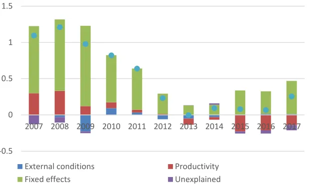
Figure 2. Decomposition of shorter-term growth (yf) by determinants in 2007-2017, sample average, in p.p. of income gap
Source: own calculations based on World bank data (available on https://wdi.worldbank.org).
5 Specification (6) does not allow to do this in a proper manner, as the estimator removes fixed effects from the model. 6 I report the results of this decomposition exercise only for the growth measured according to the ‘closing income
gap’ concept, i.e. for 4 and 4_0(, as the results for ‘standard’ growth measure are more or less the same.
-3 -2 -1 0 1 2 3 A lb a n ia A rm e n ia A ze rb a ija n B o sn ia a n d H e rz e g o v in a B u lg a ri a C ro a ti a C y p ru s E g y p t E st o n ia G e o rg ia G re e ce H u n g a ry Jo rd a n K a za k h st a n K y rg y z R e p . La tv ia Le b a n o n Li th u a n ia M a ce d o n ia M o ld o v a M o n g o li a M o n te n e g ro M o ro cc o P o la n d R o m a n ia R u ss ia S e rb ia S lo v a k R e p . S lo v e n ia T u n is ia T u rk e y Uk ra in e
External conditions Productivity Fixed effects
Unexplained YF (2007-2017 average)
-1 0 1 2
2007 2008 2009 2010 2011 2012 2013 2014 2015 2016 2017
External conditions Productivity
Fixed effects Unexplained
Shorter-term growth decomposition shows that although external environment is a ma-jor driver according to the model, not many countries enjoyed a substantial contribution from it on average basis in 2007-2017. This reflects the notion about poor room for growth due to external condition given their volatile nature. Hence, even from the perspective of short-term growth, the contribution of productivity is rather significant for many countries.
Figures 3 and 4 provide similar decomposition for a longer-term growth.
Figure 3. Decomposition of longer-term growth (yf_tr) by determinants for individual countries, 2007-2017 average, in p.p. of income gap
Source: own calculations based on World bank data (available on https://wdi.worldbank.org).
Figure 4. Decomposition of longer-term growth (yf_tr) by determinants in 2007-2017, sample average, in p.p. of income gap
Source: own calculations based on World bank data (available on https://wdi.worldbank.org).
-2 -1 0 1 2 A lb a n ia A rm e n ia A ze rb a ija n B o s& H e rz . B u lg a ri a C ro a ti a C y p ru s E g y p t E st o n ia G e o rg ia G re e ce H u n g a ry Jo rd a n K a za k h st a n K y rg y z R e p . La tv ia Le b a n o n Li th u a n ia M a ce d o n ia M o ld o v a M o n g o li a M o n te n e g ro M o ro cc o P o la n d R o m a n ia R u ss ia S e rb ia S lo v a k R e p . S lo v e n ia T u n is ia T u rk e y Uk ra in e
External conditions Productivity
Fixed effects Unexplained
YF_TR (2007-2017 average)
-0.5 0 0.5 1 1.5
2007 2008 2009 2010 2011 2012 2013 2014 2015 2016 2017
External conditions Productivity
For longer-term growth, the contribution of productivity was substantially larger than that of external conditions. At the same time, a huge contribution to growth by fixed effect should be born in mind. It signals that productivity and external conditions determinants are far from explaining growth in EM entirely. From the economic policy view, it also sig-nals that country-specific growth determinants might be also meaningful.
Figure 4 supports a widely accepted evidence of the lack of productivity gains in EM in recent years. However, jointly with Figure 3, it proves that for the whole set of EM this fact stems from very heterogeneous role of productivity in individual countries. However, countries with higher productivity gains still exhibit a higher trend growth. This sheds some more light on the phenomenon of decoupling between productivity and growth and allows to explain it within the framework where productivity is still the major growth driver.
CONCLUSIONS
The article deals with the issue of relative importance of productivity determinants vs. external conditions determinants for growth in EM. It shows that both productivity and external environment determinants are meaningful for growth in EM. However, it is crucial to differentiate between a shorter and a longer-term perspective, as the role of produc-tivity and external conditions determinants changes depending on the time-horizon. In a shorter-term, external conditions determinants are more important for growth. Here-with, external demand and financial conditions are of prior importance. Among the exter-nal environment determinants, trade conditions take up their role in a longer-term, while the role of external demand and financial condition weakens in comparison to those in a shorter-term. But in overall, productivity determinants become dominant in a longer-term. It means that productivity is still meaningful for growth and the longer the time-horizon considered, the more important productivity determinants are.
The results of this study, one the one hand, are similar to IMF (2017) and Arora and Vamvakidis (2005), as showing the importance of external conditions for growth in EM. On the other hand, they differ somehow, as stating that in a longer time-horizon produc-tivity becomes more important for economic growth, while the role of external conditions is contracting. In this part, the results of the study are more in line with Rodrick et al. (2004). Moreover, the article provides a framework where the ‘growth puzzle’ in EM – decoupling between output and TFP growth rates – can still be explained without chal-lenging the foreground role of productivity for economic growth.
From the perspective of growth-enhancing policy, the article shows that the im-portance of external conditions for EM should not lead us to incorrect belief that produc-tivity fundamentals do not matter anymore. Changes in the external environment are more likely to generate relatively short-term growth rate fluctuations, while having a mod-est impact on the sustainable growth trajectory. Hence, a country aiming to secure sus-tainable growth should still first of all think about productivity fundamentals.
stud-ies dealing with international comparisons. The evidence of the sensitivity of growth re-gressions to inclusion of productivity determinants re-echoes with Rodrick et al. (2004), and might be born in mind when exploiting the tool.
The research design of this study has got a number of limitations. First, because of data availability it deals with a relatively short time horizon and a small number of countries. Expanding the framework both in the time and space dimension might be worthwhile. Second, focusing on ‘competition’ between external conditions determi-nants and productivity determidetermi-nants, the study left out of consideration a number of alternative growth determinants. This led to leaving a substantial part of growth in EM either unexplained or assigned to country-specific/time fixed effects. Third, concen-trating on the level of growth determinants, the study does not match its effects to growth channels, which might be the contribution to the theory. Directions for future research are associated with overpassing these limitations.
REFERENCES
Acemoglu, D. (2009). Introduction to modern economic growth. Princeton, US: Princeton Unversity Press. Acemoglu, D., Johnson, S., & Robinson, J. (2001). The Colonial Origins of Comparative Development:
An Empirical Investigation. American Economic Review, 91(5), 1369-1401.
Adler, G., Duval, R., Furceri, D., Celik, S., Koloskova, K., & Poplawski-Ribeiro, M. (2017). Gone with the
headwinds: Global productivity, (IMF Staff Discussion Note 17/04). Retrieved from
https://www.imf.org/~/media/Files/Publications/SDN/2017/sdn1704.ashx on 22 October 2018. Aghion, P., & Howitt, P. (1992). A model of growth through creative destruction. Econometics,
60(2), 321-351.
Arellano, M., & Bond, S. (1991). Some tests of specification for panel data: Monte Carlo evidence and an application to employment equations. Review of Economic Studies, 58(2), 277-97. Arora, V., & Vamvakidis, A. (2005). How much do trading partners matter for economic growth?. IMF
Staff Papers, 52(1), 24-40.
Barro, R. (1991). Economic growth in a cross-section of countries. The Quarterly Journal of
Econom-ics, 106(2), 407-443.
Barro, R. (2001). Determinants of economic growth. Cambridge, Mass.: MIT Press.
Calderon, C., Loayza, N., & Schmidt-Hebbel, K. (2006). External conditions and growth performance. In R. Caballero, C. Calderon, & L. Cespedes (Eds.), External Vulnerability and Preventive Policies (pp. 41-70). Santiago, Chile: Central Bank of Chile.
Christensen L., Cummings, D., & Jorgenson, D. (1981). Relative productivity levels: 1947-1973.
Euro-pean Economic Review, 16, 61-94.
Coibion, O., Gorodnichenko, Y., & Ulate, M. (2017). The cyclical sensitivity in estimates of potential
output (NBER Working Paper No. 23580). Retrieved from
https://www.nber.org/pa-pers/w23580.pdf on 12 October 2018.
De Gregorio, J. (2018). Productivity in emerging market economies: slowdown or stagnation? (University of Chile, Department of Economics Working Paper No. 471). Retrieved from < http://econ.uchile.cl/up-loads/publicacion/38024d948e3902f952a34e0a0e968a72e4754fa7.pdf> on 15 February 2019. Edison, H., Klein, M., Ricci, L., & Slok, T. (2002). Capital account liberalization and economic
per-formance: survey and synthesis, (IMF Working Paper No. 702/120). Retrieved from <
Dollar, D., & Kraay, A. (2003). Institutions, trade, and growth. Journal of Monetary Economics, 50(1), 133-162.
EBRD. (2017). Transition report 2017-2018, London, UK: European Bank for Reconstruction and Development.
Grossman, G., & Helpman, E. (1991). Innovation and growth in the global economy. Cambridge, MA: MIT Press.
Hall, R., & Jones, C. (1999). Why do some countries produce so much more output per worker than others?. Quarterly Journal of Economics, 114(1), 83-116.
Hsieh, C., & Klenow, P. (2010). Development Accounting. American Economic Journal:
Macroeco-nomics, 2(1), 207-223.
IMF. (2015). Where are we headed? Perspectives on potential output. In IMF (Ed.), World Economic Outlook, April, 2015 (pp. 69-110). International Monetary Fund, Washington, DC.
IMF. (2016). How to get back on the fast track? In IMF (Eds.) Regional economic issues: Central,
East-ern and SoutheastEast-ern Europe, (pp. 18-47). International Monetary Fund, Washington, DC.
IMF (2017). Roads less travelled: growth in emerging markets and developing economies in a com-plicated external environment. In IMF (Eds.), World economic outlook, April, 2017 (pp. 65-120). International Monetary Fund, Washington, DC.
Kaminsky, G., Reinhart, C., & Vegh, C. (2004). When it rains, it pours: procyclical capital flows and macroeconomic policies. NBER Macroeconomics Annual, 19(2004), 11-53.
Jones, C. (2016). The facts of economic growth. In J. Taylor & H. Uhlig (Eds.), Handbook of
Macroe-conomics (pp. 3-69). Philadelphia, PA: Elsevier.
Jorgenson, D.W., Ho, M.S., & Stiroh, K.J. (2005). Growth in U.S. industries and investments in information technology and higher education. In C. Corrado, J. Haltiwanger, & D. Sichel (Eds.). Measuring capital
in the new economy (pp. 403-478). National Bureau of Economic Research, Cambridge, MA.
Klenow, P., & Rodriguez-Clare, A. (1997). The neoclassical revival in growth economics: has it gone
too far?. (NBER Macroeconomics Annual 1997, 73-114). Retrieved from
https://www.nber.org/chapters/c11037.pdf on 19 September 2018.
Kruk, D., & Bornukova, K. (2014). Belarusian Economic Growth Decomposition, (BEROC Working Pa-per No. 24). Retrieved from < http://eng.beroc.by/webroot/delivery/files/WP_24_eng_Bornu-kova&Kruk.pdf> on 15 February 2019.
Nezinsky, E., & Fifekova, E. (2014). The V4: the decade after EU entry, Entrepreneurial Business and
Economic Review, 2(2), 31-46.
Paweta, W. (2018). Impact of the international financial crisis on the business cycle in the Visegrad group, Entrepreneurial Business and Economic Review, 6(3), 43-58.
Rodrick, D., Subramanian, A., & Trebbi, F. (2004). Institutions rule: the primacy of institutions over ge-ography and integration in economic development. Journal of Economic Growth, 9(2), 131-165. Romer, P. (1990). Endogenous technical change. Journal of Political Economy, 98(5), 71-102. Solow, R. (1957). Technical Change and the Aggregate Production Function. The Review Of
Econom-ics And StatistEconom-ics, 39(3), 312-320.
Torre, L., & Colunga, L. (2015). Patterns of Total Factor Productivity Growth in Mexico: 1991-2011, (Banco de Mexica Working Paper No. 2015-24). Retrieved from
Wolff, E. (1991). Capital formation and productivity convergence over the long term. American
Eco-nomic Review, 81(3), 565-79.
Wong, W. (2001). The channels of economic growth: a channel decomposition exercise, (National University of Singapore, Department of Economics Working Paper No. 0101). Retrieved from http://www.fas.nus.edu.sg/ecs/pub/wp/ wp0101.pdf on 15 February 2019.
World Economic Forum. (2017). The global competitiveness report 2017-2018, Geneva: World Economic Forum.
Young, A. (1995) The tyranny of the numbers: confronting the statistical realities of the East Asian growth experience. Quarterly Journal of Economics, 110(3), 641-680.
Author
Dzmitry Kruk
Researcher at Belarusian Economic Research and Outreach Center (BEROC), PhD student in Cra-cow University of Economics. His research interest includes: growth and finance, growth in emerging markets, monetary policy.
Correspondence to: Mr. Dzmitry Kruk, BEROC, Gazety Pravda ave. 11-B, Minsk, 220018, Belarus, e-mail: kruk@beroc.by
ORCID http://orcid.org/0000-0003-3770-9323
Acknowledgementsand Financial Disclosure
I would like to thank Prof. Marek Dabrowski, Dr. Piotr Stanek and other participants of Interna-tional Economics Section at 4th InternaInterna-tional Scientific Conference 2018 held by Cracow Univer-sity of Economics for their helpful comments and insights.
This article has been presented as the academic paper at the scientific conference GLOB2018: “Globalization and Regionalization in the Contemporary World: Competitiveness, Development, Sustainability” organized in Kraków on 21-22 September 2019.
Copyright and License
This article is published under the terms of the Creative Commons Attribution – NoDerivs (CC BY-ND 4.0) License
http://creativecommons.org/licenses/by-nd/4.0/
Published by the Centre for Strategic and International Entrepreneurship – Krakow, Poland
The copyediting and proofreading of articles in English is financed in the framework of contract No. 913/P-DUN/2019 by the Ministry of Science and Higher Education of the Republic of Poland committed to activities aimed at science promotion.