Analysis Method for the Low-Order Resistive Interchange Instability in LHD with Stochastic Magnetic Field Line Structure

(1)

Analysis Method for the Low-Order Resistive Interchange

Instability in LHD with Stochastic Magnetic Field

Line Structure

∗

)

Ryosuke UEDA, Masahiko SATO

1)

, Kiyomasa WATANABE

1)

, Yutaka MATSUMOTO,

Yasuhiro SUZUKI

1)

, Masafumi ITAGAKI, Shun-ichi OIKAWA and Yasushi TODO

1)

Graduate School of Engineering Hokkaido University, Sapporo 060-8628, Japan

1)_{National Institute for Fusion Science, 322-6 Oroshi-cho, Toki 509-5292, Japan}

(Received 9 December 2012/Accepted 21 June 2013)

In Large Helical Device experiments, independent low-order magnetic fluctuations due to the resistive inter-change mode are commonly observed; investigating the characteristics of this instability is our ultimate goal. Two new methods for analyzing the single low-order instability in the stochastic region are developed. One method investigates it by constructing the initial single-mode perturbation. The other method investigates it by construct-ing a reference surface outside the last closed flux surface. The reference surface is necessary for constructconstruct-ing the coordinates that are used to extract the Fourier mode in the stochastic field line structure.

c

2013 The Japan Society of Plasma Science and Nuclear Fusion Research

Keywords: magnetohydrodynamics, resistive interchange mode, LHD, stochastic region, RBF expansion method DOI: 10.1585/pfr.8.2403157

1. Introduction

In high-βLarge Helical Device (LHD) experiments, independent low-order magnetic fluctuations that resonate with the rational surface are commonly observed [1]. The dependence on theβvalue and magnetic Reynolds num-ber suggests that such magnetic fluctuations are due to the resistive interchange mode. This mode is unstable in the magnetic hill region. The entire LHD plasma region typi-cally has a magnetic hill configuration with lowβ. As the

βvalue increases, a magnetic well is formed in the core region, whereas the magnetic hill remains in the peripheral region. Thus, the suppression of the resistive interchange mode in the peripheral region is thought to be important in high-βoperations. On the other hand, theoretical stud-ies predict that the structure of the magnetic surfaces is destroyed with increasingβ, and turns into the stochastic state. Therefore, to study the properties of magnetohydro-dynamics (MHD) stability in prospective LHD-type fusion reactors, it is important to investigate the characteristics of the resistive interchange mode in the stochastic magnetic ﬁeld line structure.

The interchange mode in helical-type plasma similar to that in the LHD has been studied theoretically. Many of these studies used numerical analysis codes, e.g., TERP-SICHORE [2], CAS3D [3], and NORM [4], based on the magnetic coordinates. However, to investigate the prop-erties of the resistive interchange mode in the stochas-tic region, we should use real coordinates in the MHD author’s e-mail: [email protected]

∗)_{This article is based on the presentation at the 22nd International Toki}

Conference (ITC22).

stability analysis code that handles the equilibrium with the stochastic magnetic ﬁeld line structure. Recently, the MHD Infrastructure for Plasma Simulation (MIPS) code [5, 6] was developed, and an early study of the nonlinear MHD saturation process in high-βLHD plasma was pre-sented [6]. The study predicts that the ballooning modes with a medium mode number are the most unstable and sat-urated, maintaining the pressure gradient when the plasma has a high magnetic Reynolds number. Because low-order magnetic ﬂuctuations that resonate with the rational sur-face are observed in LHD experiments, we focus on the characteristics of the resistive interchange instability with the low-order mode, which is the same as that observed in the experiments.

To analyze the independent low-order unstable mode in the stochastic magnetic field line structure, two issues must be resolved. One is the development of a method for investigating the specified single-mode instability. Al-though the original MIPS procedure employs random per-turbation of the initial conditions, this perper-turbation has multiple modes, including both stable and unstable ones. Because stable modes exist, considerable computational time is required until the growth of unstable modes ap-pear clearly. The existence of multiple unstable modes poses a problem in that we cannot investigate the speci-fied single unstable mode. In section 2, these problems are resolved by describing a single-mode perturbation in Boozer coordinates [7]. The other issue to be resolved is to define “quasi-magnetic” coordinates based on refer-ence surfaces to describe a single-mode perturbation out-side the Last Closed Flux Surface (LCFS). The use of the

c

2013 The Japan Society of Plasma

(2)

VMEC code [8] is one way to construct Boozer coordi-nates. The fixed-boundary VMEC code requires the shape of the LCFS as input. However, in the stochastic mag-netic field line structure outside the LCFS, the magmag-netic surfaces cannot be obtained by magnetic field line tracing. Without the coordinates, we cannot describe the single-mode perturbation in the stochastic field line structure. In section 3, reference closed surfaces outside the LCFS ob-tained by using the Radial Basis Function (RBF) expansion method [10] are defined. Although these reference surfaces outside LCFS are not physical, we use the surfaces as the fixed-boundary in the VMEC code to obtain Boozer-like coordinates. Using these Boozer-like coordinates, we de-scribe a single-mode perturbation outside the LCFS.

2. Development of the Initial Mode

Perturbation Method

As mentioned in the previous section, issues with the original procedure in the MIPS code need to be resolved, because this procedure cannot analyze a speciﬁed mode instability. To resolve these issues, an initial single-mode perturbation method was developed. In this method, the perturbation having a speciﬁed single unstable mode is described in Boozer coordinates. Without any other un-stable mode, the only constructed single unun-stable mode is expected to grow. In addition, without the stable mode, the linear growth of the constructed single-mode instability can be seen shortly after the beginning of the calculation, which reduces the computational time.

2.1 Method of constructing mode

perturba-tion

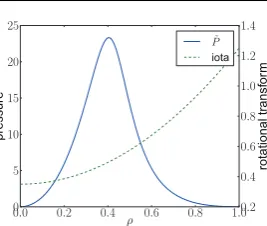
The described mode structure in Boozer coordinates is based on our knowledge of the linear analysis of the re-sistive interchange mode. The typical rere-sistive interchange mode structure of heliotron plasma is obtained by solving the eigenvalue equations based on the reduced MHD equa-tions in the straight heliotron geometry. Figure 1 shows the resistive interchange mode structure of the pressure. The poloidal mode numberm =2 and toroidal mode number

n = 1 are used. The rational surface is located around

ρ=0.4. The mode structure has a peak value around the rational surface. From this result, we model the structure of the mode perturbation in Boozer coordinates as a Gaus-sian proﬁle:

˜

P(ψ)=Aampexp

−ρ−ρs

σ

2

. (1)

HereAampis the amplitude of the perturbation, andρs

de-notes the location of the rational surface. The width of the mode structure is conditioned by theσvalue. In this study,

Aamp = 10−7 andσ = 0.05 are used. ρs depends on the

rotational transform proﬁle obtained at equilibrium. The equilibrium proﬁle is constructed by the HINT code [9]. Figure 2 shows the modeled mode structure. Because the MIPS code takes the initial conditions in real coordinates,

Fig. 1 Resistive interchange mode structure of the pressure obtained by eigenmode analysis in straight heliotron plasma.

Fig. 2 Mode structure model of pressure for the initial mode per-turbation.

Fig. 3 Mode perturbation of pressure in real coordinates in a vertically elongated cross section. Closed solid line de-notesψ=1 (ρ=1).

the mode perturbation built in Boozer coordinates is con-verted to that in real coordinates. Figure 3 shows the per-turbation on the vertically elongated cross section.

2.2 Growth of mode perturbation

The governing MHD equations in MIPS are as fol-lows:

∂p

∂t =−∇ ·(ρv)−(γ−1)p∇ ·v

+(γ−1)

νρw2+4

3νρ(∇ ·v)

2₊_η_j_·₍_j₋_j eq)

,

(2)

ρ_∂∂

tv=−ρw×v−ρ∇

v2

2

− ∇p

+j×B+4

(3)

Fig. 4 Pressure perturbation at 30,000 time steps. Magnetic Reynolds number isS=106_.

Fig. 5 Mode structures of the perturbation at 30,000 time steps. Magnetic Reynolds number isS =106_.

∂ρ

∂t =−∇ ·(ρv), (4)

w=∇ ×v, (5)

j= 1

μ0∇ ×

B, (6)

∂B

∂t =−∇ ×E, (7)

E=−v×B+η(j−j_eq). (8) The meanings of variables are the same as in Ref. [5]. The time evolution of mode perturbation was computed. The resolutions are 128×128 on the poloidal section and 256 along the toroidal direction. In the poloidal section, the computational area is set to 2.55 ≤ R ≤ 4.75 and

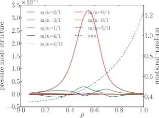
−1.1 ≤ Z ≤ 1.1. The magnetic Reynolds number andβ value areS =106andβ =2%, respectively. The initial perturbation has the single (m,n) =(2,1) mode shown in Fig. 3. Figure 4 shows the pressure perturbation at 30,000 time steps (133 Alfvén times) on the vertical cross section. It can be seen that the initial mode perturbation grows. A mode analysis of the perturbation was performed, and the perturbation proﬁle in real coordinates was mapped to Boozer coordinates. The eight largest structures of the analyzed mode are shown in Fig. 5. Among them, the (m,n)=(2,1) mode structure clearly has the largest ampli-tude. Figure 6 shows the time evolution of kinetic energy as a function of the time step. Under random perturbation

Fig. 6 Time evolution of kinetic energy. Green and blue lines denote the (2,1) mode perturbation and random pertur-bation, respectively.

(blue), the time evolution of the kinetic energy decreases until around 15,000 time steps, and then the linear growth phase appears. In contrast, under the (2,1) mode perturba-tion (green), the linear growth phase appears after around 5000 time steps. The mode perturbation is found to make the linear phase appear in fewer time steps. The rate of change of the kinetic energy depends on the growth rate. The linear growth rate under random perturbation is larger than under the (2,1) mode perturbation. Thus, random per-turbation includes various unstable modes. These include unstable modes whose growth rate is greater than that of the (2,1) mode.

3. Construction of the Reference

Sur-faces in the Stochastic Magnetic

Field Line Structure

(4)

(a) RBF cxpansion (b) Comparison between LCFS and quasi magnctic surface Fig. 7 (a) Contour map (green) and lines (red) constructed by

the RBF expansion method. (b) Comparison of LCFS (blue) and quasi-magnetic surface (green, red). One con-tour line is almost closed line (green). However, part of the line is open (red).

3.1 RBF expansion method for constructing

quasi-magnetic surfaces

Using the RBF expansion method [10], we fit the group of discrete points by tracing a magnetic field line on a poloidal cross section to a continuous curve. The curve is recognized as a quasi-magnetic surface. Within the LCFS, the curves almost coincide wth the magnetic surfaces ob-tained by magnetic line tracing. In this study, the start points of the magnetic field line tracing for the RBF ex-pansion method are

(Rstart,Zstart)=(4.0+0.01k,0), k=0,1, . . . ,70,

(9) in the horizontally elongated poloidal cross section. The magnetic field configuration at finite beta is calculated by the HINT code [9]. The centers of the RBFs are distributed on grids in the (2.2<R<5.2,−1.5<Z<1.5) region with a grid spacing ofΔ=0.3. We adopt the Gaussian function as the RBF, as in Itagaki’s study. The scaling factor of the RBF function isσ =1.0. Figure 7 (a) shows the contour map (green) and contour lines (red) obtained by the RBF expansion method.

3.2 Extracting the quasi-magnetic surfaces

for boundary geometry

Figure 7 (b) shows the larger and almost closed line (green, red) that is extracted from the contour line in Fig. 7 (a). The red line is the open part of the contour line, which is removed and interpolated so that the con-tour line becomes closed. Further, the Poincaré plot is also drawn. In particular, the blue line shows the LCFS, which is the magnetic ﬁeld line trace originating at the start point

R=4.39. Similarly, we obtain the quasi-magnetic surfaces in the stochastic region on 11 poloidal sections at toroidal angles of 0◦−18◦. However, every reference surface has to constitute the same quasi-magnetic surface. Figure 7 (b) shows that the reference surface (green line) obtained by the RBF expansion method has a larger geometry than the

Fig. 8 Boundary geometry on poloidal sections at toroidal an-gles of 0, 5.4◦, 10.8◦, and 18◦, constructed by the RBF expansion method (circles) or Fourier components in VMEC coordinates (red lines).

LCFS (blue line) and includes the region with the stochas-tic magnestochas-tic ﬁeld line structure.

3.3 Representation of the quasi magnetic

surface in VMEC coordinates

To deal with the quasi magnetic-surface as VMEC in-put, we have to represent the constructed boundary geom-etry in VMEC coordinates. The real coordinates are trans-formed to VMEC coordinates using the KFIT code, which is an improved version of DESCUR [11]. Using this code, we can obtain the Fourier representation for boundary ge-ometry. Figure 8 shows the boundary geometries obtained by the Fourier representations in VMEC coordinates (red) and those obtained by the RBF expansion method (circles) at toroidal angles of 0, 5.4◦, 10.8◦and 18◦. It can be seen that the two geometries are almost the same. The VMEC coordinates are accurately constructed outside the LCFS. Using the routine that transforms VMEC coordinates to Boozer coordinates, we can obtain Boozer-like coordinates including the stochastic region.

4. Summary

(5)

[1] K.Y. Watanabeet al., Phys. Plasmas18, 056119 (2011). [2] W.A. Copper, Plasma Phys. Control. Fusion 34, 1011

(1992).

[3] C. Nührenberg, Phys. Plasmas6, 137 (1999).

[4] K. Ichiguchi, N. Nakajima, M. Wakataniet al., Nucl. Fu-sion43, 1011 (2003).

[5] Y. Todo, N. Nakajima, M. Sato and H. Miura, Plasma Fu-sion Res.5, S2062 (2010).

[6] M. Sato, N. Nakajima, K.Y. Watanabeet al., 24th IAEA

FEC 2012, TH/P3-25 (2012).

[7] A.H. Boozer, Phys. Fluids24, 1999 (1981).

[8] S.P. Hirshman, W.I. van Rij and P. Merkel, Comput. Phys. Commun.43, 143 (1986).

[9] K. Harafujim T. Hayashi and T. Sato, J. Comput. Phys.81, 169 (1989).

[10] M. Itagaki, G. Okubo, M. Akazawaet al., Plasma Phys. Control. Fusion54, 125003 (2012).