Available online at http://www.ijabbr.com
International journal of Advanced Biological and Biomedical Research Volume 1, Issue 10, 2013: 1220-1235
Determination of Climate Changes on Streamflow Process in the West of Lake Urmia
with Used to Trend and Stationarity Analysis
Keivan KHalili 1, Farshad Ahmadi *2, Yagub Dinpashoh 3 and Ahmad Fakheri Fard 4
1
Water Engineering Department, Faculty of Agriculture, Urmia University, Urmia- IRAN, 2Msc Student of Water Engineering Department, Faculty of Agriculture, Tabriz University, Tabriz- IRAN,3 Associate Professorof Water Engineering Department, Faculty of Agriculture, Tabriz University, Tabriz- IRAN, 4 Professorof Water Engineering Department, Faculty of Agriculture, Tabriz University, Tabriz- IRAN.
ABSTRACT
One of the most important hydrological time series task is to determine if there is any trend in the data and how to achieve stationarity when there is nonstationarity behavior in data. Detecting trend and stationarity in hydrological time series may help us to understand the possible links between hydrological processes and global climate changes. In this study yearly, monthly and daily streamflow data records of Baranduz Chai, Shahar Chai and Nazlu Chai rivers and Urmia synoptic stattion in the west of Lake Urmia, located in the West Azarbaijan of Iran, used to trend and stationarity analysis. Trend analysis with Mann-Kendall and seasonal Kendall tests showed that most annual and monthly flow series had significant negative trend at 1% and 10% . Five common methods named ADF, DFGLS, ERS, KPSS and PP have been used to examine nonstationarity of river flows. Results demonstrated that most annual, monthly and daily series appear to be stationary after removing trend component from series. Also results illustrated, that mean air temperature of this region increased significantly at 1% level. Increasing air temperature causes changing most of precipitations to rain in the replace of snow that maybe the main reason of river flow decreasing and Lake Urmia depletion in recent years. Furthermore, studied rivers have high dependence on snow melt water, therefore are affected by temperature changes. This showed obviously effect of global warming on the decreasing river flow discharges in the west of Lake Urmia.
Key Words: Climate Change, Mann-Kendall test, Stationarity tests, Trend, Lake Urmia.
1. Introduction
showed that there is no obvious trend in the most of annual and monthly river discharges of Western Europe catchments in the 20th century. Although these studies examined the trends of hydrologic processes for some local regions, their because factors acting on streamflow trends on a basin scale are not necessarily similar to those acting on a regional or continental scale their extrapolations to regional or continental scale remains uncertain (Pfisher et al., 2000). Investigation on possible trend in streamflow processes seems to be related to regional climate variations and their atmospheric associations, particularly regional precipitation and temperature changes. Ghahraman and Taghvaeian (2008) demonstrate significant decreases in annual rainfall over the northwest of Iran with using the linear regression method. Dinpashoh et al.,, (2011) stablished the trends in reference crop evapotranspiration (ETO) on monthly and annual time scales in Iran and found increasing trends in monthly ETO in the northwest of Iran. Tabari and Hosseinzade (2011) found increasing trends for maximum temperature in the western half of Iran. Karaburun et al., (2011) investigated annual, seasonal and monthly temperatures in Istanbul from 1975 to 2006 and showed existence of a tendency toward warmer years. Jhajharia et al., (2012) reported negative trends in pan evaporation at annual and seasonal time scales in general for 6 sites in NE India and NE India. Annual, seasonal and monthly trends in precipitation, mean maximum and minimum temperature range were evaluated with using stations from Florida, USA by Martinez et al (2012). Results showed significant decreasing in monthly precipitation and increasing trends in mean, maximum and minimum temperature. Dibik et al., (2012) used Mann-Kendall trend analysis of precipitation and air temperature in the Lake Winnipeg watershed. They observed increasing trend in mean annual air temperature, however no significant trend in annual precipitation. Wang et al., (2012) investigated changing trends of annual mean temperature and annual precipitation over the last 50 years in Loess Plateau Region (LPR) of china. It was shown that annual mean temperature has significant increasing and annual precipitation had no-significant negative trend. Abgari et al., (2013) used non parametric methods to evaluate annual and monthly trends in river flow data from the west of Iran during the past 40 years and found downward trend in most stations (specially in October and November). Northwest of Iran (specially west of Lake Urmia), is the geographical area falls under the arid and semi-arid type of climate; however due to the agrarian is seriously vulnerable to the anthropogenic-induced climate change. It seems very likely that any changes in the availability of water adversely affect the sustainable development of agriculture and environment in northwest of Iran. However, very little information is available on trend and stationarity of streamflow processes across northwest of Iran. Therefore, the present study was conducted for three main objectives, which are as follows: (i) to detect trends in streamflow processes on daily, monthly and annual time scales of Baranduz Chai, Shahar Chai and Nazlu Chai rivers located in the West Azarbaijan with using the Mann-Kendall (MK) and seasonal Kendall (SK) tests; (ii) Testing stationarity of streamflow using the five methods which are: (1) the augmented Dickey-Fuller (ADF) unit root test, (2) Dickey-Fuller test with GLS detrending (DFGLS), (3) KPSS test, (5) Phillips-Perron (PP) test and (5) Elliot, Rothenberg and Stock Point Optimal (ERS) test; (iii) Finding any possible relationship between recent climate changes, mean air temperature and the results of trend and stationarity for streamflows in the west of Lake Urmia.
2. METHODS AND MATERIALS
2.1.Data Description
Furthermore for analyzing trend of temperature of the study area yearly and monthly data of Urmia synoptic station have been used. Details of the Urmia airport synoptic station and applied river stations are presented in Table 1.
Table1. Details of used stations in this study
Station Location Type Latitude Longitude height (m)
Time of record Start End
Dizaj Baranduz
chai river Hydrometer 37-23N 45-05E 1320 1974 2011
Mirabad Shahar chai
river Hydrometer 37-40N 44-54E 1525 1974 2004
Tapik Nazlu chai
river Hydrometer 37-26N 44-52E 1405 1974 2011
Urmia Airport Synoptic 37-32N 44-05E 1313 1974 2011
2.2.Trend analysis
The main purpose of trend analysis is to determine whether the value of a series generally increase or decrease. Nonparametric trend detection methods are less sensitive to outliers (extremes) comparing the parametric methods (such as Pearson’s correlation coefficient). In addition, a nonparametric test can test for detecting a trend in a time series without specifying whether the trend is linear or nonlinear. Furthermore, there is no need data with a certain probability distribution. Therefore, a rank-based nonparametric method, the Mann-Kendall’s test is applied in this study to streamflow time series.
2.2.1.Mann-Kendal test (MK)
Kendall (1938) proposed a measure "tau" to seek a monotonic relationship between x and y series. Mann (1945) suggested using the test significance of Kendall’s tau, where one of the variables is observations of a certain variable, which other is time as a test for trend. The test is known as Mann-Kendall’s test (referred to as MK test hereafter), which is powerful on uncovering deterministic trend. Under the null hypothesis H0, that a series { ,x x1 2,...xN}come from a population where the random variables are independent and identically distributed, the MK test statistic is:
1
1 1
sgn( )
N N
j i
i j i
S x x
(1)
Where, sgn(xixj) 1, 0
0, 0
1, 0
i j
i j
i j
x x
x x
x x
And N is the number of observations. The statistic "tau" is estimated as: 2
( 1) S N N
(2)
Kendall (1975) showed that the square root of S, for the situations may be tie (i.e., equal values) in the x values, is given by:
1 1
[ ( 1)(2 5) ( 1)(2 5)]
18
m
S i i i
i
N N N t t t
Where, m is the number of values and ti is the number of some values in the ith tied group.
Under the null hypothesis, the statistic Z defined in the following equation is approximately standard normally distributed for the sample size N>=10:
( 1) , 0
0, 0
( 1) , 0
S
S
S S
Z S
S S
(4)
If ZZ/2 then the null hypothesisH0, there is no trend in time series will be accepted. Otherwise, the H0
rejected and alternative hypothesis H1 will be accepted at α significance level. It has been found that
positive serial correlation inflates the variance of the MK statistic S and hence increases the possibility of rejecting the null hypothesis of no trend (von Storch, 1995).
2.2.2.Seasonal Kendal test (SK)
Monthly streamflow and finer time scales like 10days flow series usually exhibit strong seasonality behavior. Therefore traditional Mann-Kendall method cannot be used to examine the possible changes occur in such situations. In such a case a modified version of Kendall’s test, referred to as the seasonal Kendall test (Hirsch et al., 1982; and Slack, 1984), is used here. The seasonal Kendall test take into account the seasonality by computing the MK test on each of the p seasons separately, and combining the results. In seasonal Kendal test the overall statistic Sis computed by following equation:
1
, 1, 2,...,
p
j j
S S j p
(5)
Sj is the MK statistic (equation 1) for the season.
When serial dependence exhibit in the time series, the variance of S is defined as:
P
j
P
g P
g h
gh j
S Var S
1
1
1 1
2
)
(
(6)
Where, gh is covariance of the Kendall statistic between season g and h.
When no serial dependence detected in the time series the variance S is defined as
) (
P
j
j S Var S
1 2
(7)
The Zstatistic is approximately normally distributed and defined as:
0 ) 1 (
0 0
0 ) 1 (
S if S
S if
S if S
Z
S S
Overall tau is weighted average of p seasonal ,s, defined as:
P
j j
j P
j j
n n
1 1
(9)
where is the tau measure for season j, estimated with equation 2, and nj denotes the number of
observations without missing values for season j.
2.3.Stationary Tests
The main purpose of any stationarity test is to determine whether the mean and/or variances of observations vary with time significantly. Almost in all of the analyzing linear and nonlinear time series analysis practitioners assumed stationarity for time series. Also in most of the applications in hydrological modeling, an assumption of stationarity thus testing stationarity for justification of using those models is necessary (Salas et al.,, 1980). On the other hand, sometimes the investigation of nonstationarity may give us some insights into the underlying physical mechanism of a process. Therefore, testing for stationarity is an important topic of time series in the field of hydrology. The stationarity tests mainly carried out using the one or more of the five methods described below. It is worthy to note that these methods originated from the economic studies.
2.3.1.ADF test
Dickey-Fuller unit root tests are conducted through Ordinary least squares (OLS) estimation of regression models incorporating either an interceptor a linear trend. Consider the autoregressive AR (1) model.
t t t t y x
y . 1 t1,2,...,N (10)
Where yt is the value of streamflow at time t, N is the number of observations, xtare optional exogenous
regressors which may consist of constant or a constant and trend, and are parameters to be estimated and t are assumed to be white noise. If 1, yt is a nonstationary series and the variance of yt increases
with time and approaches infinity. If 1 then yt is a (trend) stationary series thus, the hypothesis of
(trend-) stationarity can be evaluated by testing whether the absolute value of is strictly less than one. In ADF test the null hypothesis H0 :1tested against the one-sided alternative hypothesis, i.e.
1 :
1
H . The standard DF test is carried out by estimating Equation (10) after subtracting yt-1 from the
both sides of the mentioned equation. Hence it can be written:
t t t t y x
y
. 1 (11)
1 2 1
2 2
1) . .
(
ˆ
t
N
t t N
t
t x x
x
(12)
The statistic for testing the null hypothesis that 1 is based on the usual OLS (Ordinary Least Squares) t-test as:
ˆ
ˆ 1 ˆ
ˆ
t
(13)
Where, ˆˆ is the usual OLS standard error of estimated which is defined as:
N
t t e N
t t e
x S x
S
2 2 1 2
1
2 2
1
ˆ ( )
ˆ
(14)
Where, Se denotes the standard deviation of the OLS estimate of the residuals in the regression model. Se
can be calculated as:
2 1 2
2
2 ( ˆ )
2 1
t
N
t t e x x
N
S
(15)
Dickey and Fuller (1979) derived the limiting of the statistic t under the null hypothesis ρ=1 and tables of
the percentiles of this distribution is available in Fuller (1976). The test rejects ρ=1 when t is too negative.
2.3.2.DFGLS test
Elliott et al., (1996) proposed a simple modification of the ADF tests, called as ERS in which the data are detrended so that explanatory variables are taken out of the data prior to running the test regression. ERS define a quasi-difference of yt that depends on the value a representing the specific point alternative
against which we wish to test the null:
1 1 )
(
1
t
t if if ay y
y a
y d
t t
t
t
(16)
Where, a1. Next, consider an OLS regression of the quasi-differenced data d(yt a) on the quasi-differenced d(xta):
t t
ta d x a a
y
d( ) ( ).( )
(17)
Where, xt contains either a constant, or a constant and trend. Let ˆ(a)be the OLS estimates from such
} , 1 {
} 1 {
5 . 13 1
7 1
t x
x if if T T a
t t
(18)
The DFGLS detrended data, d t
y is defined using the estimates associated with the a:
) ( ˆ
. a
x y
yd t t
t
(19)
Then DFGLS test involves estimating the standard ADF test equation and after substituting the GLS detrend d
t
y for the original yt:
t d
p t p d
t d d
t y y y u
y
t
1 1 1 ... (20)
Note that since d t
y is detrended, we do not include the xt in the DFGLS test equation. As with the ADF
test, we consider the t-ratio for aˆ from this test equation. While the DFGLS t-ratio follows a Dickey-Fuller (no constant) distribution in the constant only case, the asymptotic distribution differs when one include both a constant and trend. ERS simulate the critical values of the test statistic in this latter setting for T={50, 100, 2000, }. The null hypothesis is rejected for values that fall below these critical values.
2.3.3.KPSS test
This method has been presented by Kwiatkowski et al.,, (1992). Let{xt}, t1,2,...,N be observed series which we wish to test stationarity. Assume that we can decompose the series into the sum of a deterministic trend, a random walk and a stationary error with the following linear regression model.
t t t t r
X (21)
Where rt is a random walk, i.e.,rt rt1ut and ut is i.i.d (0, )
2
u
N ; tis a deterministic trend and tis a
stationary error. To test in this model if Xt is a trend stationary process, namely, the series is stationary around a deterministic trend. The null hypothesis will be u2 0which means that the intercept is a fixed element, against the alternative hypothesis of a positive 2
u
. In another stationarity case, the level stationarity, namely, the series is stationary around a fixed level, the null hypothesis will be 0. So that, under the null hypothesis, in the case of trend stationary, the residuals t(t=1,2,..,N) are from the
regression of x on an intercept and time trend, ett; whereas in the case of level stationarity, the
residuals etare from a regression of x on intercept only, that is etxtx . Let the partial sum process of
the et as
1
t j j
S e
, and 2be the long-run variance of et, which is defined as lim [ ]2 1 2
N
S E N
. The
consistent estimator of 2can be constructed from the residuals et by (Newey and West 1987).
2 2
1
1 1 1
1 2
ˆ ( ) ( ) .
N P N
t j t t
t j t j
P e P e e
N N
Where P is the truncation lag and wj(p) is an optional weighting function that corresponds to the choice of
a special window, e.g. Bartlett (1950) window ( ) 1 ( 1)
j
j P
P
. Then, the KPSS test statistic is given by:
N
t P
t
S N KPSS
1 2
2 2
) (
ˆ
(23)
The upper tail critical values of the asymptotic distribution of the KPSS statistic are given by Kwiatkowski et al., (1992).
2.3.4.Philips and Perron (PP) test
Phillips and Perron (1988) proposed an alternative (nonparametric) method of controlling for serial correlation when testing for a unit root. This method called here as PP method, which estimates the non-augmented DF test equation, and modifies the t-ratio of the a coefficient so that serial correlation does
not affect the asymptotic distribution of the test statistic. The PP test is based on the following statistic:
1
0 2 0 0 1
2
0 0
ˆ
( )( ( ))
ˆ ( )
2
T f se
t t
f f s
(24)
Where ˆis the estimate, and t the t-ratio of , se(ˆ)is coefficient standard error, and s is the standard
error of the test regression. In addition, 0 is a consistent estimate of the error variance in (calculated as
T S K
T 2
)
( where k is the number of regressors) and f0 is an estimator of the residual spectrum at
frequency zero. There are two choices we will have make when performing the PP test. First, we must choose whether to include a constant, a constant and a linear time trend, or neither, in the test regression. Second, we will have to choose a method for estimating f0. The asymptotic distribution of the PP
modified t-ratio is the same as that of the ADF statistic. MacKinnon (1991) reported lower-tail critical and p-values for this test.
2.3.5.ERS Point Optimal test
This method described in detaiels by Elliot et al., (1996). This method is based on the quasi-differencing regression defined in Equation (17). Residuals can be defined from Equation (17) as
) ( . ) ( ) ( ) (
ˆt a d yta d xta a
, and let SSR(a)
ˆt2(a)be the sum-of-squared residuals function. The ERS (feasible) Point Optimal test statistic of the null that a=1 against the alternative that aais then defined as:0
)) 1 ( . ) (
(SSRa aSSR f
PT
(25)
Where f0 is an estimator of the residual spectrum at frequency zero. Critical values for the ERS test
statistic are computed by interpolating the simulation results provided by Elliott et al., (1996) for T={50, 100, 2000, }.
3. RESULTS
3.1.Trend Analysis Results
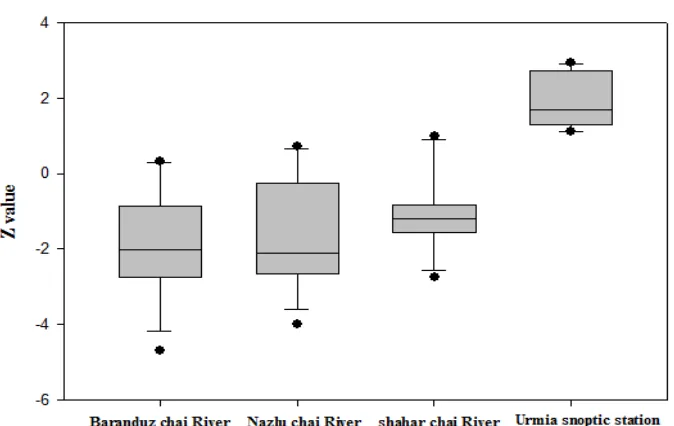
The yearly, seasonal and monthly discharge of rivers located on the west of Lake Urmia with Mann-Kendall and seasonal Mann-Kendall tests are tested. Also mean air temperature have been in order to determinate effect of global warming on river flow at the same time scales.As results showed in table 2 and figures 1 and 2, downward trend detected for annual river flow of Barandouz Chai at 5 and 10% significant level. But Shahar Chai and Nazlu Chai rivers had no significant downward trend in this time scale. For seasonal time scale, all stations showed significant negative trend at 1% level. And all monthly series exhibit decreasing trend in most months at 1 and 10% level. According to results negative significant trend observed in Barandouz-cahi river at January, March, June, July, August, September, November, December months and downward trend detected at January, June, July, August, September, November and December months in Nazlu Chai streamflow. For Shahar Chai river significant downward trend has been observed in August and September months. Mean air temperature tests showed upward trend at 1% level for both yearly and seasonal series. In monthly series, increasing significant trend at 1 and 10% levels have been observed in February, April, May, June and September.
3.2.Stationary Test Results
It is a common practice to take logs of the data before applying stationary tests (Gimeno et al., 1999). This is due to the fact that these tests are based on the linear regression, which assumes a normal distribution for data. To eliminate possible impacts of seasonality present in the streamflow processes on the effectiveness of stationarity test, besides the log transformation, data should be deseasonalized. In this study following the log transformation of the streamflow data, deseasonalization was performed. This was done by subtracting the seasonal (yearly, monthly and daily) mean values from data and dividing the results by their corresponding standard deviations. It is worthy to mention that stationary tests to the choice of lag value p are sensitive. If a small value for p selected, the remaining serial correlation in the errors will bias the test result. If p is too large, then the power of the test will suffer. Schwert (1989) and Kwiatkowski et al., (1992) proposed the Pint[ (x N 100) ]1 4 with x=4,12 for choosing the number of lag
Figure 1. Annual trend variations of studied stations
T a b le 2 . T h e r es u lt s o f M a n n K e n d a ll a n d s ea so n a l K e n d a ll t e st s o n s tr e a m fl o w a n d m e a n a ir t e m p er a tu r e se r ie
s Urm
ia s y n o p ti c st at io
n Tau 0.40 0.21 7.10 0.31 0.13 0.32 3.30 0.21 0.17 0.14 9.20 0.16 0.13 0.12
S 28
6 1 6 4 4 1 2 3 2 1 9 9
0 226 235 151 421 99 210 117 95 91
Z 3.5
8 * * 6 .2 3 * * 1 .5 3 2 .7 4 * * 1 .1 2 2 .8 2 * * 2 .9 4 * * 1 .8 8 * 1 .5 4 1 .2 3 2 .6 2 * * 1 .4 5 1 .8 2 1 .1 3 S h a h a r ch ai r iv e r T a u -0 .2 3 -0 .1 8 -0 .2 0 0 .0 0 -0 .1 3 -0 .0 8 -0 .1 6 -0 .1 4 -0 .1 9 -0 .2 8 -0 .3 5 -0 .1 0 -0 .2 4 -0 .1 9
S -16
8 -1 0 2 1 -9 0
1 56 -38 -69 -63 -88 -12
2 -1 6 3 -4 6 -1 0 8 -8 4
Z -0.9
2 -5 .0 2 * * -1 .5 8 1 .0 0 -0 .9 8 0 .6 6 -1 .2 1 -1 .1 0 -1 .5 1 -2 .1 5 * -2 .7 5 * * -0 .8 0 -1 .1 9 -1 .4 8 N az lu c h ai r iv e r T a u -0 .1 6 -0 .1 2 -0 .2 3 -0 .0 1 -0 .1 6 0 .0 8 -0 .1 6 -0 .2 8 -0 .4 5 -0 .2 7 -0 .2 9 -0 .0 6 -0 .3 0 -0 .2 5
S -11
9 -9 9 2 -1 6 2
8 -11
9 5 7 -1 0 6 -1 9 8 -3 1 8 -1 9 2 -2 0 6 -4 7 -2 1 4 -1 7 7
Z -1.4
8 -3 .7 6 * * -2 .0 2 * 0 .0 8 -1 .4 8 0 .7 1 -1 .2 9 -2 .6 7 * * -3 .9 8 * * -2 .4 0 * * -2 .5 8 * * 0 .5 8 -2 .6 7 * * -2 .2 1 * * B a ra n d u z ch ai r iv er T a u -0 .2 3 -0 .2 0 -0 .2 5 -0 .0 2 -0 .2 2 -0 .0 4 -0 .1 8 -0 .3 3 -0 .5 3 -0 .2 3 -0 .3 1 -0 .0 7 -0 .3 0 -0 .2 7
S -16
8 -1 5 9 8 -1 5 8 1
8 -159 27 -128 -236 473 -168 -222 -55 -215 -179
Z -2.1
Table3. Stationary test results for streamflow series
Rivers Series Test
parameters
Stationary Test Methods
PP test
KPSS level stationary test
KPSS trend stationary test
DFGLS test
ADF test
ERS test
Baranduz chai
Annual lag 1 1 1 1 1 1
Statistic -3.65 0.37 0.10 -3.27 -3.24 1.57
Monthly lag 8 8 8 8 8 8
Statistic -10.81 1.24 0.23 -2.85 -3.05 1.36
Daily lag 23 23 23 23 23 23
Statistic -15.78 10.18 1.51 -5.46 -9.68 0.44
Nazlu chai
Annual lag 1 1 1 1 1 1
Statistic -3.58 0.31 0.11 -2.79 -2.96 1.92
Monthly lag 11 11 11 11 11 11
Statistic -7.82 0.51 0.22 -2.26 -3.02 2.22
Daily lag 21 21 21 21 21 21
Statistic -16.73 4.45 1.82 -6.63 -9.21 0.25
Shahar chai
Annual lag 1 1 1 1 1 1
Statistic -3.54 0.22 0.07 -2.75 -2.69 1.99
Monthly lag 4 4 4 4 4 4
Statistic -7.79 0.56 0.13 -4.04 -4.36 0.59
Daily lag Statistic 26 -38.15 26 1.31 26 0.36 26 -7.10 26 -9.54 26 0.16
Note: Critical value of KPSS distribution for level stationarity hypothesis: 10% ~0.347; 5% ~0.463;
1% ~0.739; Critical value of KPSS distribution for trend stationarity hypothesis: 10% ~0.119; 5% ~0.146; 1% ~0.216.
4. Discussion
and decreasing snow storage of the studied basins. According to the river flow trend results, discharge of November December, January months and end of spring and summer decreased. This finding is in accordance with the results of Abghari et al., (2013). This was showed obviously that effect of global warming on the decreasing river flow discharge in the west of Lake Urmia.According to the results from our study, after removing trend by standardizing series, streamflow processes on all timescales became stationary. This implies that streamflow processes in the west part of Lake Urmia region are influenced by regional or even global scale. Five methods, which are ADF test (Dickey and Fuller, 1979), Dickey-Fuller test with GLS detrending (DFGLS), KPSS test (Kwiatkowski et al.,, 1992), Phillips and Perron test (1988) and Elliot, Rothenberg and Stock test (1996) were used to test for nonstationarity. Results indicated that except KPSS method all of the annual, monthly and daily series in applied methods appear to be stationary. This indicates that trend component, which has been shown by the seasonal Kendall and Mann-Kendall tests removed from series. Because of high dependency of rivers runoff located in the west of Lake Urmia on snow melt water, and temperature it can be stated that global warming is the main cause of downward trend of stuied rivers. Such downward trend for study area streamflow cause the Lake Urmia surface level decline considerably in recent years.
5. Conclusions
In this study streamflow process of Baranduz Chai, Shahar Chai and Nazlu Chai rivers at Dizaj, Mirabad and Tapik stations respectively, which located in the west of Lake Urmia, have been applied for trend and stationarity analysis. The trend of annual mean discharges was investigated using Mann-Kendall test results showed that in most stations there is obvious significant trend in annual mean discharges. Trend of monthly flow series are examined using seasonal Kendall test. Results indicated that there are significant negative trend at 1% level in all stations. In order to investigate the effect of air temperature variations and global warming on studied river flows, data of mean air temperature recorded in Urmia Synoptic station has been used. According to Tabari et al., (2011) and results of this study mean air temperature of this area increased significantly. Results of monthly and seasonally trend analysis showed decreasing in river flows happened almost one month after increasing in air mean temperature of that month. Furthermore increasing air temperature causes changing in the shape of precipitations that most of autumn and winter precipitations changed to rain in the replace of snow. In this case, evaporation from rain and rivers increases and snow storage of mountains decreases. This subject maybe the main reason of river flow decreasing and Lake Urmia depletion in recent years.Five methods concluded as ADF, Dickey-Fuller with GLS detrending (DFGLS), KPSS, Phillips and Perron and Elliot, Rothenberg and Stock tests employed to examine stationarity. Results indicated that most of the annual, monthly and daily streamflow series after removing trend became significantly stationary. This indicates that there is trend component in streamflows, which detected by the seasonal Kendall and Mann-Kendal tests. It was concluded that nonstationarity of streamflow in daily and monthly time scales might be the effect of climate change on streamflow in the study area.
6. REFERENCES
Abghari, H., Tabari, H., Talaee, P.H., 2013. River flow trends in the west of Iran during the past 40 years: Impact of precipitation variability. J of Hydrology, 101:52-60.
Balling, R.C.J.r., 1992. The Heated Debate: Greenhouse Predictions versus Climate Reality. Pacific Research Institute for Public Policy, San Francisco, 195 pp,.
Birsan, M., Zaharia, L., Branescu, E., and Chendes, V., 2008. Trends in Romanian Stream Flow over the Second Half of the 20th Century. Geophysical Research Abstracts, 10: EGU 2008 – A – 10880, 1607 – 7962.
Burn, D.H., and Hag Elnur, M.A., 2002. Detection of Hydrologic Trends and Variability. Journal of Hydrology, 255: 107-122.
De Wit, M.J.M., 2001. Effect of Climate Change on the Hydrology of the River Meuse. Report 104, Wageningen University, Environmental Sciences, Netherlands.
Dibike, Y., Prowes, T., Shrestha, R., Ahmed, R., 2012. Observed trends and future projections of precipitation and air temperature in the Lake Winnipeg watershed. Journal of Great Lakes Research, 38(3):72-82.
Dickey, D.A., and Fuller, W.A., 1979. Distribution of the Estimators for Autoregressive Time Series with a Unit Root. Journal of American Statistical Association.
Dinpashoh, Y., Jhajharia, D., Fakheri-Fard, A., Singh, V.P., and Kahya, E., 2011. Trends in reference crop evapotranspiration over Iran. Journal of Hydrology, 399: 422–433. DOI:10.1016/j.jhydrol.2011.01.021.
Elliott, G., Thomas, J., Rothenberg, J., and Stock, H., 1996. Efficient Tests for an Autoregressive Unit Root. Econometrica, 64:813-836.
Ghahraman, B., and Taghvaeian, S., 2008. Investigation of annual rainfall trends in Iran. Journal of Agricultural Science and Technology, 10:93–97.
Gimeno, R., Manchado, B., and Mingues, R., 1999. Stationarity Tests for Financial Time Series. Physica. A, 269(1): 72-78.
Hirsch, R.M., Slack, J.R., and Smith, R.A., 1982. Techniques of Trend Analysis for Monthly Water Quality Data. Water Resources Research, 18(1):107-121.
Hirsch, R.M., and Slack, J.R., 1984. A Nonparametric Trend Test for Seasonal Ddata with Serial Dependence. Water Resources Research, 20(6):727-732.
Jhajharia, D., Dinpashoh, Y., Kahya, E., Singh, V.P., and Fakheri-Fard, A., 2012. Trends in reference evapotranspiration in the humid region of northeast India. Journal of Hydrological Processes, 26:421-435. DOI: 10.1002/hyp.8140.
Kahya, E., and Kalayci, S., 2004. Trend Analysis of Streamflow in Turkey. Journal of Hydrology, 289:128-144.
Karaburun, A., Demirci, A., and Kara, F., 2011. Analysis of Spatially Distributed Annual, Seasonal and Monthly Temperatures in Istanbul from 1975 to 2006. World Applied Sciences Journal, 12 (10): 1662-1675.
Karla, A., Piechota, T.C., Davies, R., and Tootle, G.A., 2008. Changes in U.S. Streamflow and Western U.S, Snowpack. Journal of Hydrologic Engineering ASCE, 1084-069.
Kendall, M.G., 1938. A New Measure of Rank Correlation. Biometrika, 36: 81-93.
Lettenmaier, D.P., Wood, A.W., Palmer, R.N., Wood, E.F., and Stakhiv, E.Z., 1999. Water Resources Implications of Global Warming, A U.S. Regional Prespective. Clim. Change, 43: 537-579.
Lins, H.F., and Slack, J.R., 1999. Streamflow trends in United States. Geophysical Research Letters, 26(2): 227-230.
MacKinnon, J.G., 1991. Critical values for cointegration tests. Chapter 13 in R.F. Engle and C.W.J. Granger (eds), Long-run Economic Relationships: Readings in Cointegration, Oxford University Press.
Martinez, C.J., Maleski, J.J., Miller, M.F., 2012. Trends in precipitation and temperature in Florida, USA. J of Hydrology, 453:259-281.
Mann, H.B., 1945. Nonparametric test against trend. Econometrica, 13: 245-259.
MCCabe, G.J., and Wolock, D.M., 2002. A step Increase in Streamflow in the Conterminous United States. Geophysical Reasearch Letters, 29 (24): 2185.
Newey, W.K., and West, K.D., 1987. A simple, positive semi-definite, heteroskedasticity and autocorrelation consistent covariance matrix. Econometrica 55: 703-708.
Pfister, L., Humbert, J., and Hoffmann, L., 2000. Recent trends in rainfall-runoff characteristics in the Alzette River Basin, Luxembourg. Climatic Change, 45(2):323 – 337.
Phillips, P.C.B., and Perron, P., 1988. Testing for a unit root in time series regression. Biometrika, 75: 335-346.
Said, S.E., and Dicky, D., 1984. Testing for Unit Roots in Autoregressive Moving Average Models with Unknown Order. Biometrika, 71: 599-607.
Salas, J.D., Delleur, J.W., Yevjevich, V., and Lane, W.L., 1980. Applied Modeling of Hydrologic Time Series. Water Resources Publications, Littleton, Colorado.
Shin, Y., and Schmidt, P., 1992. The KPSS Stationarity Test as a Unit Root Test. Economic Letters, 38: 387-392.
Schwert, G.W., 1989. Test for Unit Roots: A Monte Carlo Investigation. Journal of Business and Economics Statistics, 7: 147-159.
Tabari, A., and Hosseinzadeh-Talaee, P., 2011. Recent trends of mean maximum and minimum air temperatures in the western half of Iran. Journal of Meteorological Atmosphere Physics, 111:121–131.
Van Gelder, P., Kuzmin, V., and Visser, P., 2000. Analysis and Statistical Forecasting of Trends of Hydrological Processes in Climate Changes. In: Proceedings of the International Symposium on Flood Defence, Vol. 1 (Toensmann F. and Koch M., Eds.), Kassel, Germany, pp D13-D22.
Von Storch. H., 1995. Misuses of Statictical Analysis in Climate Research. In: Analysis of Climate Variability: Applications of Statistical Techniques, (Storch HV and Navarra a Eds), Springer Verlag, New York, pp. 11-26.
Wang, Q., Fan, X., Qin, Z., Wang, M., 2012. Change trends of temperature and precipitation in the Loess Plateau Region of China, 1961–2010. Global and Planetary Change, 93: 138-147.
Westmacott, J.R., and Burn, D.H., 1997. Climate Change Effects on the Hydrologic Regime within the Churchill-Nelson River Basin. Journal of Hydrology, 202: 263-279.