University of Pennsylvania
ScholarlyCommons
Publicly Accessible Penn Dissertations
1-1-2015
Dynamics and Statics of Liquid-Liquid and
Gas-Liquid interfaces on Non-Uniform Substrates at the
Micron and Sub-Micron Scales
Michael Meredith Norton
University of Pennsylvania, [email protected]
Follow this and additional works at:http://repository.upenn.edu/edissertations
Part of theChemical Engineering Commons,Mechanical Engineering Commons, and the Physics Commons
This paper is posted at ScholarlyCommons.http://repository.upenn.edu/edissertations/1921 For more information, please [email protected].
Recommended Citation
Norton, Michael Meredith, "Dynamics and Statics of Liquid-Liquid and Gas-Liquid interfaces on Non-Uniform Substrates at the Micron and Sub-Micron Scales" (2015).Publicly Accessible Penn Dissertations. 1921.
Dynamics and Statics of Liquid-Liquid and Gas-Liquid interfaces on
Non-Uniform Substrates at the Micron and Sub-Micron Scales
Abstract
Droplets and bubbles are ubiquitous motifs found in natural and industrial processes. In the absence of significant external forces, liquid-liquid and gas-liquid interfaces form constant mean curvature surfaces that locally minimize the free energy of a given system subject to constraints. However, even for sub-micron bubbles and droplets free of hydrodynamic and hydrostatic stresses (small Capillary, Weber, and Bond numbers), non-equilibrium at the contact line of sessile bubbles and droplets can influence geometries and dynamics. First, the wetting of micron-sized ellipsoidal particles was considered. In the space of axially symmetric interfaces, it is found that multiple constant mean curvature surfaces can satisfy volume and contact angle constraints. Partial encapsulation may be preferred even when the droplet's volume is sufficient to fully engulf the particle. The co-existence of multiple equilibrium states suggests possible hysteretic encapsulation behavior. Secondly, motivated by electron microscopy observations of sub-micron bubbles in a liquid cell, a small mobile and growing bubble confined between two weakly diverging plates is considered theoretically. Scaling analysis suggests that observed bubbles move by continuously wetting and de-wetting the substrates onto which they are adhered. 2D and 3D models are constructed incorporating the Blake-Haynes mechanism, which relates the dynamic contact angle to contact line velocity; partial pinning of the contact line is also considered. In 2D, the system is fully described by a set of non-linear ordinary differential equations that can be readily solved. In 3D, the non-linear PDE system and constraints were solved using a pseudo-spectral method. Both 2D and 3D models predict that in order for a doubly confined bubble to grow in a super-saturated solution it must first increase its curvature; this is in contrast to a free-floating bubble whose curvature always decreases with the addition of mass/volume. Since the surface concentration is proportional to the internal pressure of the bubble, this geometric change temporarily regulates the growth of the bubble. The model predicts growth rates like those observed experimentally that are several orders of magnitude lower than predictions made by classical mass transfer driven growth theory developed by Epstein and Plesset.
Degree Type Dissertation
Degree Name
Subject Categories
DYNAMICS AND STATICS OF LIQUID-LIQUID AND GAS-LIQUID INTERFACES ON NON-UNIFORM SUBSTRATES AT THE MICRON AND SUB-MICRON
SCALES
Michael M. Norton
A DISSERTATION
in
Mechanical Engineering and Applied Mechanics
Presented to the Faculties of the University of Pennsylvania
in
Partial Fulfillment of the Requirements for the
Degree of Doctor of Philosophy
2015
Supervisor of Dissertation
______________________________
Haim H. Bau
Professor, Mechanical Engineering and Applied Mechanics
Graduate Group Chairperson
______________________________
Prashant K. Purohit
DYNAMICS AND STATICS OF LIQUID-LIQUID AND GAS-LIQUID INTERFACES ON NON-UNIFORM SUBSTRATES AT THE MICRON AND SUB-MICRON
SCALES
COPYRIGHT
2015
Acknowledgements
To all my friends and family and those listed by name below, this
accomplishment is yours as much as it is mine. First and foremost, I want to thank my
parents Robert and Sharon Norton for their love and tremendous support throughout my
studies.
I want to thank my advisor, Dr. Haim Bau, for offering his perspective and
insights as I developed my ideas through the years and for creating the environment that
made this work possible. Dr. Howard Hu, for generously offering his knowledge
throughout my time as a student and for serving on my committee. Dr. Kathleen Stebe,
for sharing her enthusiasm and passion for research with me, in addition to serving on my
committee. I want to thank my academic parents, Dr. Risa Robinson and Dr. Steven
Weinstein for their support and advice that surely brought me to where I am today.
Special thanks to Dr. Frances Ross for welcoming me into the world of electron
microscopy and creating a positive, nurturing environment in which to develop my ideas.
Dr. Calvin Li, for offering an honest perspective on academia and for enthusiastic support
of my research.
Thanks to the entire faculty and staff of the department of Mechanical
I owe many thanks to my academic cohorts in the Bau-Hu lab and Dr. Daeyeon
Lee’s lab for their conversations, and willingness to share their resources and technical
expertise. In particular, I’m gracious for my friendships with Steven Henry, Nicholas
Schneider, and Joe Grogan. Their day-to-day conversation and support helped me grow
intellectually and gain perspective on integrating academia, research, and life.
I feel deeply fortunate to have met many artists and craftspeople outside of
academia during my time in Philadelphia. In particular, I want to thank Ann Klicka,
Kimberly Shelton, Andy Upright, Leslie Grossman, Nathanial Ross, Matt Gilbert, Mike
Rossi and Chris Winterstein for their friendship and for welcoming me to a whole new,
inspiring world and offering their unique perspectives.
I am indebted to Laura Finch, Marta Mackiewicz, Eva Wô, and Katy Hardy.
Through their dedicated friendship, love, and wisdom, I gained perspective on my studies
and myself; I learned how to prioritize personal health in the face of daunting projects. I
hope that I can love and champion them and others around me in the same way. Finally, I
want to thank my lifelong friends Dan Boardman, Van Johnson, and Spencer Shultz for
their loyalty and support all these years.
This work was supported, in part, by the National Science Foundation (NSF)
NSEC DMR08-32802 through the University of Pennsylvania's Nano-Bio Interface
ABSTRACT
DYNAMICS AND STATICS OF LIQUID-LIQUID AND GAS-LIQUID INTERFACES ON NON-UNIFORM SUBSTRATES AT THE MICRON AND SUB-MICRON
SCALES
Michael M. Norton
Haim H. Bau
Droplets and bubbles are ubiquitous motifs found in natural and industrial
processes. In the absence of significant external forces, liquid-liquid and gas-liquid
interfaces form constant mean curvature surfaces that locally minimize the free energy of
a given system subject to constraints. However, even for sub-micron bubbles and droplets
free of hydrodynamic and hydrostatic stresses (small Capillary, Weber, and Bond
numbers), non-equilibrium at the contact line of sessile bubbles and droplets can
influence geometries and dynamics. First, the wetting of micron-sized ellipsoidal
particles was considered. In the space of axially symmetric interfaces, it is found that
multiple constant mean curvature surfaces can satisfy volume and contact angle
constraints. Partial encapsulation may be preferred even when the droplet's volume is
sufficient to fully engulf the particle. The co-existence of multiple equilibrium states
suggests possible hysteretic encapsulation behavior. Secondly, motivated by electron
considered. In 2D, the system is fully described by a set of non-linear ordinary
differential equations that can be readily solved. In 3D, the non-linear PDE system and
constraints were solved using a pseudo-spectral method. Both 2D and 3D models predict
that in order for a doubly confined bubble to grow in a super-saturated solution it must
first increase its curvature; this is in contrast to a free-floating bubble whose curvature
always decreases with the addition of mass/volume. Since the surface concentration is
proportional to the internal pressure of the bubble, this geometric change temporarily
regulates the growth of the bubble. The model predicts growth rates like those observed
experimentally that are several orders of magnitude lower than predictions made by
Table of Contents
Acknowledgements ... iii
ABSTRACT… ... v
Table of Contents ... vii
List of Tables ... ix
List of Figures ... x
Chapter 1. Background ... 1
Chapter 2. The Geometry of Droplets on Ellipsoids ... 4
2.1. Motivation ... 4
2.2. Materials and Methods ... 6
2.2.1. Fabrication of Elongated Polystyrene Particles ... 6
2.2.2. Encapsulation of Elongated Polystyrene Particles ... 8
2.3. Image Processing ... 10
2.4. Mathematical Model ... 12
2.5. Results and Discussion ... 15
2.6. Conclusion ... 26
Chapter 3. Liquid-‐Gas Interface Observations in SEM and TEM ... 28
3.1. Motivation ... 28
3.2. Experimental Methods ... 30
3.3. Initial Observations of Sub-‐Micron Bubbles in TEM ... 35
3.4. Bubble Transport Hypotheses ... 40
3.5. “Sliding” Sphere Model ... 46
3.6. Growth Anisotropy Revisited ... 50
Chapter 4. Bubble Growth in Hele-‐Shaw Devices ... 53
4.1. Motivation ... 53
4.2. Governing Equations and Scaling ... 57
4.3. Contact Line Dissipation ... 62
5.7. Spectral Representation ... 92
5.8. Initial Conditions ... 95
5.9. Model Results ... 96
5.9.1. Volume Controlled Case ... 96
5.9.2. Partially Pinned Bubble – Volume Controlled ... 104
5.9.3. Mass Transfer Driven Growth ... 107
5.10. Conclusions ... 112
Chapter 6. Growing Sessile Bubble with Contact Line Dissipation ... 114
6.1. Motivation ... 114
6.2. Insoluble ... 114
6.3. Compressible and Soluble ... 122
6.4. Conclusion ... 131
Chapter 7. Conclusions and Outlook ... 132
Chapter 8. Appendix ... 141
8.1. Drop Shape Calculation Using Numerical Energy Minimization ... 141
8.2. Contact Angle Measurement ... 147
8.3. Dimensionless Groups ... 147
8.4. How Ellipsoidal are the Particles? ... 149
List of Tables
Table 5.1: The magnitudes of the various properties used in the calculation of Table 5.3.The light mineral oil’s manufacturer provides the kinematic viscosity at 40oC
while the specific gravity is given at 15.6oC. Subscripts CE and PS, respectively, denote properties of the C.elegans and polystyrene ... 148
Table 5.2: Typical velocity and length scales. Subscripts D, CE, and PS denote properties belonging to a typical droplet, C.elegans, or polystyrene particle. ... 149
List of Figures
Fig. 2.1: The ellipsoidal particles’ formation process. (A) The creation of a polystyrene emulsion using a flow-focusing apparatus. (B) Evaporation of solvents from the emulsion in a warm water bath. (C) A micrograph of solidified mono-dispersed spheres. (D) Embedding PS particles in a PVA film. (E) Stretching of the heated PVA film to elongate the particles. (F) Dissolution of PVA film in water to release the ellipsoidal particles. (G) A micrograph of the ellipsoidal particles. ... 8
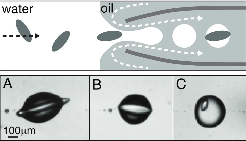
Fig. 2.2: A schematic (top) of the encapsulation process and (bottom) three typical encapsulation results. (A) a partially encapsulated particle, (B) a nearly fully engulfed particle in an ellipsoidal drop, and (C) a fully encapsulated particle in a spherical drop. ... 9
Fig. 2.3: (Left) A photograph of an elongated polystyrene particle (σ) partially
encapsulated in a water drop (α) and suspended in a continuous phase (β) of oil. The interface is computed with the unduloid solution (dashed line) and energy
minimization (hollow circles). The particle aspect ratio ε=8.0±0.9, the dimensionless volume V*=0.027±0.007, and the contact angle θ =10°. The ellipsoid’s major (a) and minor (b) axes, the droplet’s radius (r2), and the axial position of the pinning line (z1) are shown. (Right) The schematic details of the discretized domain used in the energy method. The radial position (ρ) originating from the spheroid’s center, the inclination angle (φ), the arc length (l), and the node number (n) are shown. The discretization is used in the energy method. See supplement. ... 11
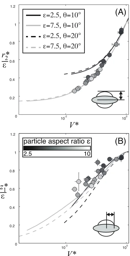
Fig. 2.4: The dimensionless maximum droplet radius r2*/ε =r2 /a (A) and the axial position of the contact line 1 1
*/ /a
z ε =z (B) as functions of the volume !!V*.
Experimental data points (circles) are color-coded according to their aspect ratio. Black indicates a stubby particle; the lighter the color, the more slender the particle. The theoretical predictions are depicted for two aspect ratios, ε=2.5 (gray line) and 7.5 (black line), and two contact angles, !θ=10° (solid line) and
!θ =20° (dashed
line). ... 17
Fig. 2.5: Contours of constant contact angle θ and constant volume V*are depicted in the space of the unduloid coefficients
( )
* 1
r
χ
and * 2r ; ε =3. Regions I (white
background) and II (gray background) correspond, respectively, to drop volumes
* 1
V < and V* >1. The hollow (red) circle denotes the smallest fully engulfing, spherical drop with V* =1. The solid dots indicate the maximum possible
unduloidal drop volume at a given contact angle. ... 19
Fig. 2.6: The shapes of the two solution branches (V* =1.20, solid lines) and that of the
limiting drop (V* =1.34, red line). θ =60° and ε =3. ... 22
Fig. 2.8: A magnified image of the framed region in Fig. 7. ΔE*(A) and * 1
z (B) are depicted as functions of V*. θ =60° and ε =3. The arrows describe a gedanken
experiment. ... 25
Fig. 2.9: Normalized curvature (A) and axial force (B) as functions of dimensionless volume; ε =3. Hollow circle denotes a spherical, engulfing drop. ... 26
F 32
Fig. 3.2: (Left) Total cell thickness and (Right) slope as a function of dimensionless position where a is the half-width of the membrane !!a=50µm (the origin is at the center of the membrane) for !!P/Patm=10−2,10−1,100!and!10. ... 33
Fig. 3.3: Intensity profiles from two STEM images (inset) before (bottom) and after (top) bubble creation converted to water thickness (asterisks and circles correspond, resptively, to before and after bubble creation) compared to the Maier-Schneider theory[79]. Estimated pressures were respectively ~1/7 and ~1/2 of an atmosphere. ... 33
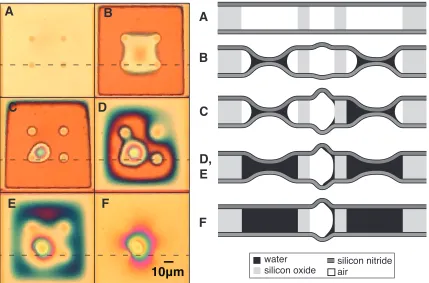
Fig. 3.4: (Left) Light microscope images of the silicon nitride membrane at various stages of liquid cell filling and (Right) a schematic of the cross-section along the dashed line (not to scale, deformations are exageratted for clarity). Color variations are due to height variatons that result in constructive and destructive interference of different wavelengths. (A) Unfilled liquid cell. (B-C) Capillary action pulling the windows together, and trapping an air bubble. (D-F) After adding liquid to the ports, the membranes spontaneoulsly relax, note that the bubble’s projected area increases. ... 35
Fig. 3.5: Composite image created from several TEM images observed at a magnification of 5,000X. All images are unaltered to illustrate the difference between vignetting and larger scale transmission gradients. Each still is !!1.8[µm]
across. ... 38
Fig. 3.6: (Right) TEM image of an empty liquid cell and (Left) the same image with enhanced contrast, illustrating vignetting. ... 38
Fig. 3.7 : Trajectories of bubbles observed at three different nanoaquarium locations. (A – top) and (B - middle) are observations made at 5,000x, (C - bottom) is at 10,000x. ... 39
Fig. 3.8: A typical bubble and its intensity profile taken along the principal axes and the direction of motion. Markings on intensity profile illustrate the drop in background intensity that occurs across the length of the bubble. ... 43
view, bright field TEM images, and intensity profiles taken along the principal axis. ... 46
Fig. 3.11: Translational velocity !x! as a function of growth rate of the hydraulic radius !R!
for bubbles observed at 10,000x (gray “+”) and 5,000x (gray dots) magnifications. A bubble at each magnification is hilighted (connected points) along with its moving average trajectory in
!
!
{ }
R!,x! space. Solid and dashed lines are, respectively, eqn.[3.3] (Fig. 3.10.C) and eqn. [3.4] (Fig. 3.10.A). !θ0=45°.
!ϕ=10−1,10−1.25,10−1.5! .
... 49
Fig. 3.12: Contact-line and centroid evolution of a bubble that nucleated in the field view. At early times the bubble grows while the position of the rear portion of the contact line changes very little; the last several frames show a sudden change in behavior. To show the passage of time, early profiles are plotted with more
transparency.!!Δt=1/15!s. ... 52
Fig. 3.13: Measured translational velocity (symbols) as a function of (A) bubble’s hydraulic radius and (B) as a function of aspect ratio. N=23. Data symbol’s size is proportional to the hydraulic radius. The solid lines in (A) correspond to !!x!~RH
and !!x!~10RH. Solid arrow in (B) indicates the passage of time. ... 52
Fig. 4.1: Schematic of 2D bubble slug showing contact line positionsx±, contact angles
θ
±, local channel half-height !h±, radius of curvature R, half-length L, and centerposition X with exaggerated taper ϕ. ... 64
Fig. 4.2: θ− (red) and θ+ (black) contact angle evolution (A) when the wedge angle
!ϕ=
{
0.1,0.3,0.5,0.7}
(!!V0* =0.004 and
!θ0=45
°) and (B) when the area flux
! !V0
* =
{
0.001,!0.002,!0.01,!0.02}
(!ϕ=0.25 and !θ0=45°). ... 71
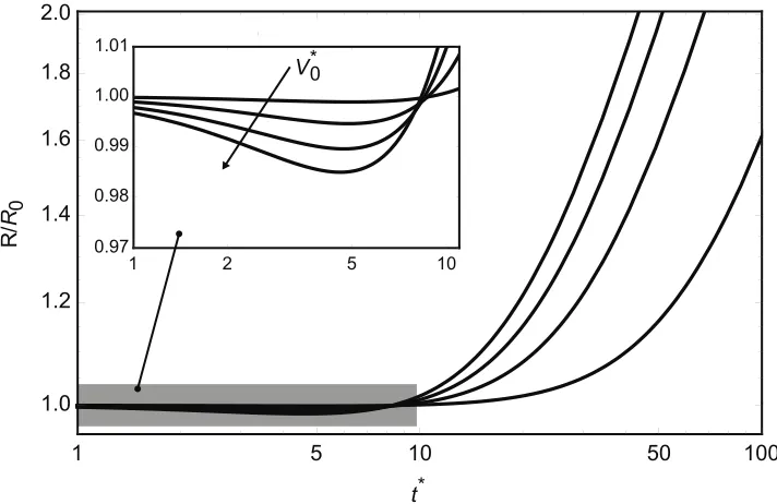
Fig. 4.3: Bubble radius of curvature normalized by starting radius as a function of time.
! !V0
* =
{
0.001,!0.002,!0.01,!0.02}
.!ϕ=0.25 and !θ0=45
°. ... 72
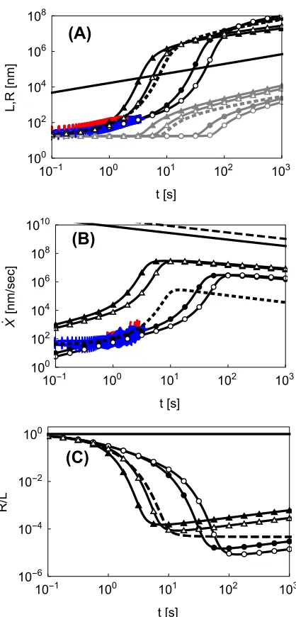
Fig. 4.4: Bubble half-length and radius (A), velocity (B), and ratio R/L (C) as functions of time. The blue “+” and red dots represent experimental data from, respectively, 10,000x and 5,000x observations. We plot four combinations of !ηCLand ϕ:
!
!ηCL=η0{10
1,103} are respectively, triangles and circles; and
!ϕ=10−6,10−6.25 are
respectively solid and hollow symbols. Dashed lines correspond to
!
!ηCL,−→ ∞ . Solid
and dashed lines are Epstein-Plesset theory using eqn. [3.3] for the velocity with
!ϕ=10−6and !10−6.25 (note that the growth rates are nearly identical while the
velocities differ). In (B), black trends are the half-length L and gray trends are t he corresponding radius of curvature R. !η0=8.9×10⁻⁴!Pa!s,
!
!h0=15!nm, !α =−4, !!θ0=30
°, and
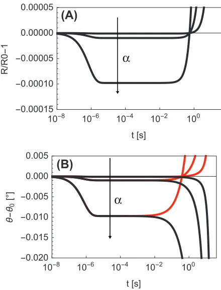
Fig. 4.5:!!R/R0−1 (A) and !θ±−θ0 (± are, respectively, black and red) (B) as functions of time.
!α=
{
−2,−3,−4}
. !!ηCL=η0103 and ϕ=10−6. All other parameters are the
same as in Fig. 4.4. ... 76
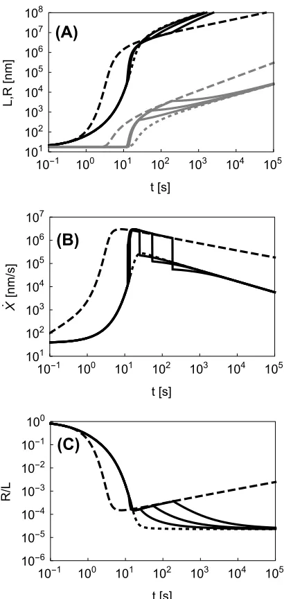
Fig. 4.6: Bubble half-length and radius of curvature (A), velocity (B), and ratio R/L (C) as functions of time. Blake-Haynes model !!ηCL=η0103 (dashed), pinned rear contact
line
!
!ηCL,−→ ∞(dotted), and hysteresis with!!βA=
{
1.10,1.15,1.20}
and !!βR=1 (black,from left to right) results. For all trends, !α =−4!ϕ=10−6. ... 78
Fig. 5.1: Problem schematic, top view. Solid curve is the contact line, dashed curve is the bubble geometry at the mid-plane of the wedge. ... 85
Fig. 5.2: Coefficient evolution (n=1,2…N) normalized by the 0th order mode for three different truncations (N=3,4,5). In the long time limit, the contact line assumes a perfectly circular geometry regardless of where the series was truncated. Different line styles correspond to the three different N used (see key); coefficents (n) are labeled. ... 98
Fig. 5.3: Relative Error !R,!Xand!ρ0(1st, 2nd, and 3rd rows, respectively) for N=0,1,2,3,4 compared to N=5 (
!
!Error=
(
fN−f5)
f5 ). Left column shows temporal evolution ofthe error and in the right column, gray scale indicate time (from light to dark,
!
!t=10−1,101,103,105 ). ... 99
Fig. 5.4: (Left Column) Temporal evolution of bubble center !X, average contact line radius !ρ0, and radius of curvature !Rand (Right Column) their time derivatives for
!
!V0= 1×10
−3,5×10−3,1×10⁻²
{
}
; values correspond to curves from bottom to top in all plots. ... 101Fig. 5.5: Temporal evolution of the ratio between the radius of curvature !R and the 0th mode !ρ0 that governs the average radius of the droplet. The droplet begins as a sphere (the initial ratio being dictated by the contact angle and wedge angle eqn. [5.37]) but becomes more “squashed” as time goes on. Under volume controlled cases !!V*∝V
0
*t3, a geometric steady state of self-similar growth is reached. From
top to bottom
! !V0
*=
{
1×10−3,5×10−3,1×10⁻²}
. As noted when describing the initialcontact line normalized by the average radius !ρ0 and centered around !X, note that a larger time range is used (!!t=0,100,200!500) for the !Φ=0.01 case to illustrate that the same elongated geometry of !Φ=0.1 is approached. !θ0=45° ... 107
Fig. 5.9: Comparison between 2D model (dotted line) presented in Chapter 4 and 3D model (solid line) of (A) Bubble size (half length L for 2D model or !ρ0 for 3D model), (B) velocity, and (C) radius of curvature R for a few different wedge angles,
!Φ= 10
−4,10−5,10−7
{
}
. Growth is driven by mass transfer.!
!η=η010
3,α=−3,h
0=15[nm] ... 109
Fig. 5.10: Contact line evolution comparison between experiment (data points) and mass transfer driven model (lines) with partial contact line pinning (A) and without it (B), darker lines and points correspond to later times. Values that provided the best fit to the experimental data are !!Φ=10−6.3,η=η
010
2,α=−2.73,h
0=15[nm], time between
frames !!Δt=0.2[s]. ... 110
Fig. 5.11: Comparison between 2D model with (gray, dotted line) and without (black, dotted line) a pinned rear contact line, 3D model with and without contact line pinning (respectively, gray and black solid lines), and the experimental data of 7 bubbles that nucleated at the same location. (A) Bubble size (half length L for 2D model or !ρ0 for 3D model), (B) velocity, and (C) radius of curvature R for mass transfer driven growth!!Φ=10−6.3,η=η
010
2,α=−2.73,h
0=15[nm], these are the
same values that provided the best fit in Fig. 5.10. An open, gray circle marks the end of the predictions made by the pinned, 3D model. ... 111
Fig. 6.1: Schematic of a spherical sessile bubble (white) of radius !R with a contact angle
θ (as measured from the liquid side, gray). ... 116
Fig. 6.2: (A) radius of curvature, (B) contact angle and (C) contact line radius of an incompressible droplet growing according to !!V*=V
0 *t*3 ,
! !V0
* =
{
10−2,10−1,!1,!10,102,103}
. At !!t≫1 , !R∝t (dotted line) and !θ →! 0 (larger growth rates are associated with steady state values further from equilbrium).
!θ0=45
° ... 117
Fig. 6.3: (A) radius of curvature, (B) contact angle and (C) contact line radius of an incompressible droplet initiated at a non-equilibrium contact angle and relaxing toward its equilbrium state while conserving volume, !!V0*=0. All droplets are given
the same initial volume such that the final radius of curvature of the equiliberated droplet !!R*=1.
!θ0=45
°
. ... 120 Fig. 6.4: (A) Contact angle evolution of a droplet beginning at a non-equilibrium contact
angle while conserving volume !!V0* =0. Trends compare full model (black line) and
linearized model (eqn. [6.7]) (gray dashed line) for
!
!θi= 30
°,60°
(B) Relaxation time constant !λ1 (eqn. [6.8]) as a function of initial contact angle for
!θ0= 45
°,90°,135°
{
}
... 121Fig. 6.5: A sample of the mesh (with !θ0=45°) used for the finite element calculation of
the total mass flux into the bubble plotted in Fig. 6.6. The bubble has unit radius, the actual domain size used was 50 times the size of the bubble. ... 123
Fig. 6.6: Comparison of the (dimensionless) mass flow into a sessile bubble as a function of contact angle between a spherically symmetric solute field (black line) and a more realistic calculated using the finite element method (black points). Note that when the bubble is a perfect hemisphere (!θ =90° ) the two methods agree due to
symmetry. ... 124
Fig. 6.7: (A) radius of curvature, (B) contact angle and (C) contact line radius of a shrinking bubble
!Ω2= 10
−4,10−3,10−2,10−1,1,10
{
}
.!α=1.1,!!P∞*=0.01 and!Ω1=0.019. ... 126 Fig. 6.8: (A) radius of curvature, (B) contact angle and (C) contact line radius of a
bubble whose surface concentration matches the concentration in the solute initially
!α=1, but begins with a non-equilibrium contact angle, !θ
( )
0 ={
1°,15°,30°}
. Thebubbles grow; however, the contact angle evolution is non-monotonic., !θ0=45°,
!
!P∞=0.01, !Ω1=0.019 and !Ω2=10
−3. ... 127
Fig. 6.9: (A) radius of curvature, (B) contact angle and (C) contact line radius of a shrinking bubble
!α =
{
0.999,0.99,0.9}
. Solid, dotted, and dashed lines are,respectively !Ω2→0, !Ω2=10 −5 and
!Ω2=10
−4. !
!P∞
*=0.01!and!Ω
1=0.019. ... 128
Fig. 6.10: (A) radius of curvature, (B) contact angle comparison between theory mass transfer driven theory and the experimental work of Li et al.[106]
!Ω2= 1,10
−1,10−2,10−3,0
{
}
, !θ0=160° ... 130Fig. 7.1: An SEM micrograph of a large bubble oscillating in the nanoaquarium liquid cell. The bubble is oscillating at approximatley 100 Hz. Because of the slow scan speed of the microscope, the bubble oscillates several times while the image is captured. ... 138
Fig. 8.2: The axial position of the pinning line (A) and the drop radius r2*/ε =r2/a (B) as functions of the dimensionless volume V*. The solid lines and the symbols
denote, respectively, the unduloid solution and the energy minimization solution.
ε=5 and θ =90°. ... 146
Chapter 1.
Background
Droplets and bubbles are ubiquitous motifs found in natural and industrial
processes; as such, interest spans multiple fields within engineering, physics, and
mathematics. At the micro- and nano- scale multi-phase systems are of interest to
developers of droplet-based high-throughput lab-on-chip devices and meta-materials built
up from emulsions and colloids[1]-[3]. In these applications, the immiscibility of two
phases is utilized to either transport a disperse phase (typically water) of a well-controlled
size containing reactants or specimens of interest within a carrier fluid (typically mineral
or silicon oil), or to provide an interface for colloidal assembly.
In all these cases, the geometry of the solid, the volume of the disperse phase, and
the contact angle determine the shape of the liquid-liquid interface or gas-liquid interface
and ultimately the behavior of the system. Clever conduit design in drop-based devices
can induce the merging of bubbles and droplets, or incite instabilities forcing them to
dispense from a fluid stream or divide. Colloids can be made to jam on a confined
interface and create non-spherical, stabilized emulsions[4], or the curvature of the
at the contact line can critically alter the behavior of the system[9]-[12]. Contact line
physics also impact colloidal adsorption to interfaces [13] and are important for
deposition of Langmuir-Blodgett films [14].
In this thesis, interface geometry, interface-substrate interactions, and contact line
dynamics will be explored in two different systems where capillary forces dominate over
viscous, inertial, and body forces. In Chapter 2, the geometry of sub-millimeter droplets
of water adhered to ellipsoidal polystyrene particles of comparable size will be examined.
It will be shown that when a substrate is finite and curved, that multiple interface
geometries can exist for a given volume of the disperse phase. However, it is found that
because these configurations are geometrically disparate, the system can exhibit
conformational hysteresis. Theory shows that if one begins with a small droplet bound to
the particle and increases its volume the system will evolve through one set of geometries
while if one begins with a droplet that fully engulfs the ellipsoid and shrinks it, a different
set of geometries will be accessed. Chapter 3 focuses on novel electron microscopy
observations of growing and moving sub-micron bubbles created by
electron-beam-induced radiolysis [15], [16] and confined within a Hele-Shaw-like apparatus comprised
of a micro-fabricated pressure vessel designed to enable imaging with electrons [17].
Chapter 4 will illustrate how classical theories describing bubble growth[18]-[21] are not
applicable under the conditions encountered in Chapter 3 and need to be modified to
explicitly account for the interplay between contact line dynamics [9]-[12], confinement,
and mass transfer. It will be demonstrated by developing a 2D model based on the
Blake-Haynes model for contact line movement [12] that the restricted movement of the contact
curvature increase with volume at short time scales. Chapter 5 will expand on the
intuition gained from the 2D model to develop a 3D model valid for highly confined high
aspect ratio bubbles (bubbles whose height is much less than their projected radius). The
model is able to predict the contact line shapes observed experimentally and confirms the
important role of pinning at early times. Chapter 6 examines a theoretically simpler but
still important scenario of a bubble on a single substrate growing and shrinking due to
diffusion with the same contact line resistance model used in the previous chapters.
Model predictions show that, unlike the doubly-confined cases considered in Chapters 4
and 5, growth is relatively unaffected. However, for a dissolving bubble, it is shown that
as contact line resistance is increased, dissolution can be inhibited and the bubble
temporarily stabilized; the model can be thought of as a generalization to the completely
pinned nanobubbles modeled by Lohse and Zhang [22]. This work closes in Chapter 7
with suggestions for further theoretical work on bubbles that move by contact line
wetting and de-wetting and hi-lights two ostensibly beam-induced interfacial fluid
dynamical phenomena relevant to liquid cell electron microscopy: interface oscillations
Chapter 2.
The Geometry of Droplets on Ellipsoids
2.1.
Motivation
Rapid and controllable encapsulation of colloidal objects in aqueous drops is
useful for high throughput studies of bacteria [23], [24], cells [25], embryos [26], [27],
and larger multi-cellular organisms such as nematodes [28]. High throughput devices
confer the opportunity to efficiently explore the effects of genetic and environmental
factors on phenotype. The same encapsulation method can also be used to form
anisotropic colloidal materials with customized properties. This work is motivated by our
work on encapsulating Caenorhabditis elegans (C. elegans) in water drops dispersed in
oil, using a flow-focusing platform similar to the one described in Utada et al. [29].
It was observed that, under certain conditions, the animals were partially
encapsulated and under others, fully encapsulated. C. elegans are compliant and deform
under the action of surface tension forces. To gain insights into the encapsulation process,
it is desirable to examine separately the effect of particle’s size and elasticity. Hence, it
was advantageous to study a simpler system of rigid particles. To estimate the importance
of elasticity in the particle-droplet system, we compare the capillary force resulting from
the pinned contact line to the critical load required for Euler-buckling [30]. The ratio of
these two forces is given by the dimensionless group Γ=
(
8γa2cosθ) (
/ π2Eb3)
, whereE, γ, a, b, and θ are, respectively, the elastic modulus, surface tension, minor particle
study, we focus on polystyrene particles with Γ~O(10−7
). In contrast, Γ~O(106
) for
live C. elegans. By focusing on rigid particles, we are able to examine geometric effects
in the absence of elastic ones.
In the absence of gravitational forces, the oil-water interfaces belong to a special class of
axisymmetric, constant curvature solutions of the Young-Laplace equation known as
unduloids or Delaunay surfaces [31]. Princen[32], Roe [33] and Carroll[34] were the first
to apply the unduloidal solutions of the Young-Laplace equation to the cylindrical
fiber-wetting problem. The pinning of droplets and bubbles on patterned substrates have
attracted ongoing interest from both experimentalists and theorists [35]-[40]. In
particular, Hanumanthu and Stebe determined the equilibrium positions and stability of
droplets pierced by a cone[41] and Michielsen[42] experimentally confirmed that droplet
equilibrium positions coincided with the free-energy minima. None of the above studies
has considered finite length particles that can be either partially or fully encapsulated by
the drop.
In this chapter, the shape of axisymmetric drops encapsulating ellipsoidal
particles as a function of drop volume, contact angle, and particle dimensions is
determined. I discuss experimental results and extend Carroll’s classical fiber wetting
exist: a spherical engulfed state and two pinned, unduloidal states. For one pinned
solution branch, the distance of the contact line from the particle’s center increases as the
droplet volume increases. For the other pinned solution branch, counter to intuition, the
opposite is true; the axial pinning position retracts upon droplet volume increase. While
not energetically favorable, this second barrel configuration possesses a lower mean
curvature and lower internal pressure than the first. As the droplet volume is increased,
the two solution branches eventually coalesce at a limit point that signifies the end of the
existence of axially symmetric pinned solutions. Further volume increases result in either
the breaking of axial symmetry (which we do not consider in this work) or a fully
engulfed state. We gain further insights into the problem by calculating the system’s free
energy as a function of state, which reveals the existence of hysteretic behavior.
2.2.
Materials and Methods
2.2.1.
Fabrication of Elongated Polystyrene Particles
Polystyrene spheres were formed (Fig. 2.1) with a flow-focusing device constructed
from glass capillaries in the same manner as Utada et al. [29]. A solution of polystyrene
(Scientific Polymer Products, Inc., Mw 190,000, CAS: 9003-53-6, CAT: 845) 15% w/w
dissolved in a solvent, comprised of chloroform 75% v/v (Fisher Science, CAT: C606)
and toluene 25% v/v (Fisher Science, CAT: T290), was flowed into the device at a flow
rate of Qinner =300µl/hr to form the dispersed phase (Fig. 2.1.A). The outer phase
13000-23000 (Sigma Aldrich, CAT: 363170) that helped stabilize the polystyrene
emulsion and was pumped in at a rate Qouter =10,00µl/hr. The emulsion was discharged
into a 40oC water bath. The solvents evaporated, and the drops solidified to form
~ 100µmdiameter spheres (Fig. 2.1.C).
To form elongated particles, we followed a process previously described in [43]-[48].
Briefly, the particles were embedded in a liquid film of PVA (87-89% hydrolyzed Mw
85,000-124,000, Sigma Aldrich CAT 363081) dissolved in water. Evaporation of the
water yielded a solid, free-standing film of PVA (Fig. 2.1.D) embedded with the PS
particles. The film was subsequently clamped into a pulling apparatus, heated to above
the glass transition temperature of polystyrene (~100oC), using a handheld heat gun, and
pulled (Fig. 2.1.E). The applied tension caused the particles to elongate and assume
nearly ellipsoidal shapes. While under tension, the film and particles were cooled to room
temperature, rendering the particles’ deformations permanent. The PVA film was then
dissolved in water to release the now ellipsoidal particles. The particles were washed
multiple times by exchanging the water suspending them to remove excess PVA. The
so-formed ellipsoidal particles varied significantly in their sizes, which required us to
individually measure the dimensions of the particles with which we experimented. Fig.
angle, and droplet morphology also depend strongly on the surfactant concentration. The
contact angle measurement is described in supplemental information.
Fig. 2.1: The ellipsoidal particles’ formation process. (A) The creation of a polystyrene emulsion using a flow-focusing apparatus. (B) Evaporation of solvents from the emulsion in a warm water bath. (C) A micrograph of solidified mono-dispersed spheres. (D)
Embedding PS particles in a PVA film. (E) Stretching of the heated PVA film to elongate the particles. (F) Dissolution of PVA film in water to release the ellipsoidal particles. (G) A micrograph of the ellipsoidal particles.
2.2.2.
Encapsulation of Elongated Polystyrene Particles
The encapsulation of the polystyrene ellipsoids took place in a flow-focusing device
similar to the one used to create the polystyrene spheres. Fig. 2.2(top) depicts a
Polystyrene Solution
water
PVA
PVA
w.
w.
A
B
D
E
F
100μm
G
schematic of the encapsulation process. Polystyrene ellipsoids were first imbibed into a
length of vinyl tubing from a dish containing rinsed particles. The tube was subsequently
connected to a syringe pump at one end and to the flow-focusing device at its other end.
The suspension was then discharged through the device. The jet (central stream) laden
with the particles was sheathed with a co-stream of immiscible oil. Observations were
carried out using an inverted optical microscope (Nikon Diaphot 300) at 4×
magnification; encapsulation events were captured at 10,000-15,000 frames per second
with a high-speed SR-CMOS camera (Phantom V7.1). Fig. 2.2(bottom) shows three
typical encapsulation results: (A) a partially encapsulated particle, (B) a nearly fully
engulfed particle in an ellipsoidal drop, and (C) a fully encapsulated particle in a
spherical drop.
water
oil
2.3.
Image Processing
The encapsulated particles were imaged while in the flow focusing device (Fig.
2.2). The images of the encapsulated particles were processed with ImageJ and Matlab to
deduce the droplet volume, the position of the pinning line, the maximum radius of the
droplet, and the particle dimensions.
In ImageJ, the oil-water interfaces were traced using the multi-point tool as
schematically depicted on the right hand side of Fig. 2.3. The top and bottom profiles of
each projection of an encapsulated particle were traced out in five consecutive frames
and the center, inclination, major axis (a), and minor axis (b) were determined. We found
that the particles can be approximated reasonably well as prolate ellipsoids with the
averages of a and b serving, respectively, as the major and minor axes. See the Appendix
for a discussion of the accuracy of this approximation. The ellipsoid’s aspect ratio
/ 1
a b
ε = > . The volume of the drop V was estimated using trapezoidal integration of the
discretized droplet surface.
We present our experimental data and theoretical predictions with dimensionless
quantities. The minor radius b is the length scale. The droplet’s dimensionless equatorial
radius and contact line position are, respectively, r2* =r2/b and *
1 1/
z =z b. The volume
of the drop (V) is normalized with the volume V0 of the smallest spherical drop that
encapsulates the particle. In other words,
(
3 2)
0 4 3
V = π a −ab is the difference between
the volume of a sphere of radius a and the ellipsoid’s volume. The dimensionless volume
*
The measurements of the interface geometry were adversely affected by optical
aberrations resulting from the difference in the indices of refraction of the glass, water,
and mineral oil and the device’s circular geometry. Specifically, the encapsulated
particles appeared smaller in width than their true size. To minimize errors from this
distortion, we used the exposed ends of the polystyrene particle for the ellipsoid fitting.
This method worked well for the partially encapsulated particles, but posed a challenge
when the particles were nearly fully encapsulated since there was little polystyrene-oil
interface available for curve fitting.
Fig. 2.3: (Left) A photograph of an elongated polystyrene particle (σ) partially
encapsulated in a water drop (α) and suspended in a continuous phase (β) of oil. The
interface is computed with the unduloid solution (dashed line) and energy minimization
(hollow circles). The particle aspect ratio ε=8.0±0.9, the dimensionless volume
V*=0.027±0.007, and the contact angle θ =10°. The ellipsoid’s major (a) and minor (b)
l
φ
n100
μ
m
n=N
n=1 z1
r2 r1
α
β
β
σ
ρ
ασ;nρ
αβ;na
b
2.4.
Mathematical Model
In this section, we describe the calculation of the axisymmetric encapsulating drop’s
shape. We consider three incompressible domains: a rigid elongated particle σ, a droplet
α, and continuous phase β (Fig. 2.3). Since the Bond number 2
2
| | /
Bo= ρβ −ρα gr γαβ,
the capillary numberCa=µβU /γαβ, and the Weber number We U2D/
β αβ
ρ γ
= are all on
the order of 0.1 or less (see Appendix I), we assume the droplet to be at a uniform
pressure. In the above, ρ ~O
(
103kg m/ 3)
is the fluid density; g is the gravitationalacceleration; r2 ~O
(
100µm)
is the maximum droplet radius; γαβ ~O mN m(
1 /)
is theinterfacial surface tension between phases α and β; ~O
(
10 3Pa s)
β
µ
− ⋅ is the viscosity;(
)
~ 1D O mm is the diameter of the glass capillary, and U O mm s~
(
1 /)
is the averagefluid velocity. Clean oil/water interfaces have an interfacial tension ~O
(
10mN m/)
[49],but the addition of surfactant may lower this number by an order of magnitude [29], [50].
To determine the interface between the drop (α) and continuous phase (β) we employ
two different methods. The first method takes advantage of the pressure uniformity inside
the drop under equilibrium conditions and in the absence of external fields (Bo<<1). The
Young-Laplace equation implies that the interface αβ must have a constant mean
curvature. The corresponding axisymmetric surfaces are, therefore, unduloids or
Delaunay surfaces [31]. The interface can be specified by a general transcendental
( )
( )
( )
2 2 2 2 2 2 2 2 1 21 sin cos
, 1 sin sin
, ,
r k u v
u v r k u v
ar F k u r E k u
⎧ − ⎫ ⎪ ⎪ ⎪ ⎪ =⎨ − ⎬ ⎪ + ⎪ ⎪ ⎪ ⎩ ⎭ r [2.1]
at the particle’s center. The position vector is parameterized by the unduloid’s surface
parameter u and the azimuthal angle v. Bold and italic print letters denote, respectively,
vectors and scalars. The functions F and E are, respectively, the incomplete elliptic
integrals of the first kind and second kind. The modulus
2 2 2 1 1 r k r χ ⎛ ⎞ = −⎜ ⎟ ⎝ ⎠ , where 2 1 2 1 cos cos u u r r r r ϕ χ ϕ − = − .
In the above, r1 is the radius of the ellipsoid at the contact line; r2 is the major radius of
the unduloid; and ϕu is the angle that the unduloid’s surface makes with the z-axis. The
contact angle θ ϕ ϕ= u − e, where
1 arctan e z r z ϕ = ⎡⎢−∂∂ ⎤⎥ ⎢ ⎥
2 1 1 1
a z r =b −⎜ ⎟⎛ ⎞
⎝ ⎠ . [2.3]
The unduloid parameter at the pinning line
u1=
arcsin 1 k 1− r1 r2 " # $ % & ' 2 " # $ $ % & ' ' ( ) * * * + ,
-when 0≤ϕu ≤π
π −arcsin 1
k 1− r1 r2 " # $ % & ' 2 " # $ $ % & ' ' ( ) * * * + ,
-when π ≤ ϕu≤2π 1 2 3 3 3 3 4 3 3 3 3 5 6 3 3 3 3 7 3 3 3 3
. [2.4]
Equation [2.4] together with the equation
(
2)
(
2)
1 , 1 2 , 1 1
r F k u r E k u z
χ + = [2.5]
enable us to determine u1 and r2.
Our second solution strategy minimizes the system’s free energy subject to a volume
constraint by discretizing the drop’s surface and finding the stationary state. The energy
minimization technique can handle more general circumstances than addressed here. In
the interest of space, the description of the energy method is deferred to Appendix I. The
energy method yielded identical results to the ones obtained when assuming unduloidal
2.5.
Results and Discussion
We start by comparing the predicted shape of the drop-oil interface with the
experimentally observed one. Fig. 2.3 (LHS) overlays the theoretical predictions (dashed
line - unduloid surface, and hollow circles - energy minimization) on top of the
experimentally observed drop, partially encapsulating an ellipsoidal particle with aspect
ratio ε =8.0 0.9± . The droplet’s dimensionless volume is V*=0.027 0.007± and the
contact angle θ =10°. Although a couple of small droplets are visible in the background,
they do not appear to distort the shape of the interface. Both theoretical predictions are in
excellent agreement with each other (<3% root mean square difference) and in good
agreement with the experimental data (<13% root mean square discrepancy).
Fig. 2.4.A and B depict, respectively, the drop’s dimensionless radius *
2
r (at the
symmetry plane z=0) and the dimensionless axial position of the pinning line *
1
z as
functions of the dimensionless volume V*. The lines and circles denote, respectively,
theoretical predictions and experimental data. The four curves featured in Fig. 2.4
correspond to permutations of two aspect ratios, ε=2.5 (black line) and 7.5 (gray line),
and two contact angles, θ =10° (solid line) and 20° (dashed line). Error bars represent
insensitive to the precise value of the contact angle. The predictions for * 1
z exhibited a
greater dependence on the contact angle θ. As V* increased, so did *
2
r and *
1
z . For a
fixed volume, the greater the hydrophilicity (the smaller the contact angle) is, the smaller
the droplet radius *
2
r and the greater the distance to the pinning line ( *
1
z ) are. Generally,
the theoretical predictions are in reasonable agreement with experimental observations.
The average root mean square discrepancies between the predicted and experimentally
observed *
2
r and *
1
z values are, respectively, 3% and 9%. A significant source of error is
due to the volume estimate that is calculated as the product of three measured linear
dimensions. Additionally, when the particles are long (ε>>1) and the drops small ( V*
<<1), the free-energy varies slowly with the pinning position ( *
1
z ), causing a lengthy
relaxation time [42]. An experimental error would result when the approach to
equilibrium occurs over a time interval that exceeds the observation time in our dynamic
experiments [13]. Yet another complication is potential wettability gradients along the
particles’ surfaces, resulting from non-uniform surfactant absorption and particle
Fig. 2.4: The dimensionless maximum droplet radius r2*/ε =r2 /a (A) and the axial
position of the contact line z*/ε =z /a (B) as functions of the volume *.
10-2 100 0
0.2 0.4 0.6 0.8 1 1.2
10-2 100 0
0.2 0.4 0.6 0.8 1 1.2
V*
10 2.5
particle aspect ratio ε
ε=2.5, θ=10° ε=7.5, θ=10° ε=2.5, θ=20° ε=7.5, θ=20°
(A)
(B)
V*
z*
1r*
2Next, we predict behaviors that are not readily accessible experimentally. Fig.
2.5 depicts the relationship among various parameters that characterize the unduloid. All
variables are dimensionless, and the particle’s aspect ratio ε =3. The abscissa and
ordinate are spanned, respectively, by
( )
*1
r
χ
and *2
r . The various solid curves correspond
to the specified contact angles. The dashed lines correspond to the drop’s volume. For
example, when the drop has volume V* =0.05 and contact angle θ =60°, *
2 1.51
x = and
*
1 0.29
x
χ =− . Regions I (white) and II (gray) correspond, respectively, to drop volumes
* 1
V < and V* >1. In the latter case, the volume is sufficiently large to allow a spherical
drop to fully engulf the particle. The hollow (red) circle represents the state when the
drop has a spherical shape, V* =1, *
1 0 r = , *
2
r =ε, and the particle is fully engulfed. See
the inset next to the hollow circle. All constant contact angle curves emanate from the
hollow circle since as *
1
z →ε, V* →1, indicating that all unduloids approach a spherical
configuration in this limit. The region *
1 0 r
χ < corresponds to situations when χ <0 (
* * 1 2 cosϕu <r r/ ).
Fig. 2.5 shows that, for each contact angle, there is a maximum volume *
max
V that
can be supported by an unduloidal drop. The unduloids corresponding to *
max
V are
denoted with solid (red) dots and can be found explicitly by determining
( )
*1
r
χ
and *2 r
( )
( )
( )
1 2 1
2 1 2 d d d V V r r dV r r r r θ θ θ χ χ χ ∂ ∂ ⎡ ⎤ ⎢∂ ∂ ⎥⎧ ⎫ ⎧ ⎫ ⎢= ⎥ ⎨ ⎬ ⎢ ∂ ∂ ⎥⎨ ⎬ ⎩ ⎭ ⎢ ⎥⎩ ⎭ ∂ ∂ ⎣ ⎦ [2.6]
becomes singular for a given contact angle. When * *
max
V >V , the drops are spherical and
completely engulf the particle (i.e., Fig. 2.2.C).
extended 180º 150º 90º 60º 30º 0º 0.05 0.50 1.00 1.50 2.00
I
II
retractedr*χ
1
-1.0 -0.5 0.0 0.5 1.0
When !!V*<1 , Fig. 2.5 illustrates that there is only one possible unduloidal drop
configuration for any given drop volume and contact angle. When V* >1, multiple
unduloidal drop configurations are possible, however. Witness that, when V*>1 and
0
θ > , constant volume curves intersect constant contact angle curves twice. In other
words, there are three possible axisymmetric drop configurations: two consisting of
partial engulfment (the right and left insets at the top of Fig. 2.5) and one of complete
engulfment (Fig. 2.2.C). To obtain further insight into the two possible partially engulfed
configurations, Fig. 2.6 depicts the two unduloids when θ =60° and V* =1.2 (solid
lines). We include in the figure also a third unduloid having the limiting volume
* 1.34
max
V = (θ =60°, dashed line). We refer to this unduloid as the limiting drop. This
third unduloid corresponds to the red solid dot in Fig. 2.5. For better visibility, we
enlarge the region next to the contact line in the inset. We refer to the drop
configurations to the left and right of the limiting drop as the retracted and extended
branches, respectively. Let’s consider a gedanken experiment in which one gradually
increases the drop’s volume. As the drop volume increases, both the contact lines
associated with the retracted and extended branches approach the position of the drop
with the limiting volume. The contact line of the retracted branch migrates away from the
particle’s center, increasing the particle’s wetted area, as we observed in the experiments.
Counter to intuition, the extended drop contracts as its volume increases. The extended
configuration always has a lower curvature than the extended branch. To determine
which branch is preferred, we will consider the surface energy of each configuration.
In addition to the two axisymmetric pinned, barrel states (B) and the fully engulfed
as an axially-asymmetric clam-shell (C-S) [36] and an expelled (EX) state in which the
particle resides entirely in the continuous phase, outside the drop. In this paper, we have
restricted ourselves to axisymmetric configurations, and we cannot comment on possible
transitions to the C-S state. We will compare, however, the free energies of the various
axisymmetric states. We use the expelled state as the reference state (state of zero
energy). Fig. 2.7 depicts the dimensionless free-energies
( )
ΔE* of the pinned states(solid lines) and, when admissible, of the engulfed states (dotted lines) as functions of the
volume V* for various contact angles θ. The particle’s aspect ratio ε =3. We use γb2 as
the energy scale. We identify three regions. In region I (V*<1), only one pinned
axisymmetric conformation is possible. In region II (1 * *
max V V <
< , shaded area), full
encapsulation (dashed line) and two pinned solutions (solid lines) are possible. The two
pinned solution branches meet at V* =1. The lower and upper, pinned branches
correspond, respectively, to the retracted and extended states. The retracted state is a state
of lower energy than the extended state. In region III ( * *
max
V >V ), no pinned solutions are
possible. When θ<70°, the pinned, retracted state is the lower energy state while the
engulfed and expelled states are metastable. When θ >70°,expulsion is the preferred
Fig. 2.6: The shapes of the two solution branches (V* =1.20, solid lines) and that of the
limiting drop (V* =1.34, red line). θ =60° and ε =3.
To better clarify the energy landscape in region II, Fig. 2.8.A magnifies the region
enclosed in the dotted rectangular frame of Fig. 2.7 (θ =60°). Fig. 2.8.B depicts the
position of the pinning line when the drop is pinned ( *
1
z <ε, * * max
V <V , solid lines) and
the radius of the engulfing spherical drop (when V* >1 , dashed line). Let’s consider a
hypothetical experiment in which one gradually increases the volume of the drop from
state A. When V*<1, only the pinned, retracted state (solid line) is possible (see inset
next to A). Once V* exceeds one, an additional pinned state, an extended state (solid
red), and an engulfed state (dashed line) becomes possible. In the gray region (
* * *
1<V <VC =Vmax), three states coexist. When 1 * *
B
V V
< < , the pinned, retracted state is
the state of lowest energy. When * *
B
V =V (state B), the engulfed and pinned states have
the same energy. When * * *
B V C
V < <V , the engulfed state is energetically most favorable.
r*
z*
1.0 2.0 3.0
0.0
0.0 1.0 2.0 3.0
1.20
1.20 1.34
0.1 0.2 0.4
0.02.8 2.9 3.0 3.1 0.3
Point C is a limit point at which the retracted and extended pinned branches meet. When
* * C
V >V , only the fully engulfed state exists. In the hypothetical experiment, one would
anticipate that when the drop volume is gradually increased, the pinned, retracted state
would persist until * *
D
V =V . Further increase in volume will induce a discontinuous
transition to the engulfed state (D). If one were to gradually decrease the drop volume
from state (D), the system would likely follow a different path, a path of engulfed states,
up to state (E) before jumping discontinuously to the pinned state (F). The “extended”
pinned branch, which provides an alternative route between (C) and (E), is likely
inaccessible. In the above, we described a potential hysteretic behavior in which the
system follows different paths in the directions of increasing and decreasing volumes
when 1 * *
max V V < < .
I II III
180º 150º 120º
90º
60º
0º 30º
V*
0.0 1.0 2.0 3.0
Δ
E*
0
Next, we examine the axial force that the drop applies on the particle
( )
(
)
{
}
* * * *
1 1
2 cos 1
z u
F =−π r ϕ + −r κ . [2.7]
In the above, κ* =bκ is the dimensionless uniform curvature (twice the mean curvature)
of the drop. Fig. 2.9.A depicts the normalized curvature as a function of the normalized
volume V* for various contact angles. The force is normalized with bγαβ. The first term
in eq. 8 is the force exerted by the contact line on the particle. This force can be either
compressive or tensile depending on the magnitude of the angle of the tangent to the
drop’s surface ϕu. The second term in [2.7] results from the Laplace pressure acting on
the particle’s surface. This force is always compressive in the case of a prolate
ellipsoid. Fig. 2.9.B depicts the axial force *
z
F as a function of the droplet volume V*
for several contact angles. Positive and negative *
z
F represent, respectively, tension and
compression. When the drop is wetting (θ <90°), the contact line exerts a compressive
force. When θ >90°, tensile force is possible. The transition from compression to tension
occurs when the pinning line force balances the compressive force due to the pressure in
Fig. 2.8: A magnified image of the framed region in Fig. 7. ΔE*(A) and * 1
z (B) are
depicted as functions of V*. θ =60° and ε =3. The arrows describe a gedanken
experiment.
A
B C
D E
F
A
D
C E
F
B
I
II
III
ΔE*
2.2 3.0 3.4
3.2
2.4 2.8
2.6
2.0
0.6 0.8 1.0 1.2 1.4 1.6
-7.8 -7.0 -6.6
-6.8
-7.6 -7.2
-7.4
-8.0
0.6 0.8 1.0 1.2 1.4 1.6