A Systematic Study of Online Class Imbalance Learning with Concept Drift

(1)

A Systematic Study of Online Class Imbalance

Learning with Concept Drift

Shuo Wang,

Member, IEEE,

Leandro L. Minku,

Member, IEEE,

and Xin Yao,

Fellow, IEEE

Abstract—As an emerging research topic, online class im-balance learning often combines the challenges of both class imbalance and concept drift. It deals with data streams having very skewed class distributions, where concept drift may occur. It has recently received increased research attention; however, very little work addresses the combined problem where both class imbalance and concept drift coexist. As the first systematic study of handling concept drift in class-imbalanced data streams, this paper first provides a comprehensive review of current research progress in this field, including current research focuses and open challenges. Then, an in-depth experimental study is performed, with the goal of understanding how to best overcome concept drift in online learning with class imbalance.

Index Terms—Online learning, class imbalance, concept drift, resampling.

I. INTRODUCTION

With the wide application of machine learning algorithms to the real world, class imbalance and concept drift have become crucial learning issues. Applications in various domains such as risk management [1], anomaly detection [2], software engi-neering [3], and social media mining [4] are affected by both class imbalance and concept drift. Class imbalance happens when the data categories are not equally represented, i.e., at least one category is minority compared to other categories [5]. It can cause learning bias towards the majority class and poor generalization. Concept drift is a change in the underlying distribution of the problem, and is a significant issue specially when learning from data streams [6]. It requires learners to be adaptive to dynamic changes.

Class imbalance and concept drift can significantly hinder predictive performance, and the problem becomes particularly challenging when they occur simultaneously. This challenge arises from the fact that one problem can affect the treatment of the other. For example, drift detection algorithms based on the traditional classification error may be sensitive to the imbalanced degree and become less effective; and class im-balance techniques need to be adaptive to changing imim-balance rates, otherwise the class receiving the preferential treatment may not be the correct minority class at the current moment. Although there have been papers studying data streams with an imbalanced distribution and data streams with concept drift

S. Wang and X. Yao (the corresponding author) are with the Centre of Excellence for Research in Computational Intelligence and Applications (CERCIA), School of Computer Science, The University of Birmingham, Edgbaston, Birmingham B15 2TT, UK. X. Yao is also with the Department of Computer Science and Engineering, Southern University of Science and Tech-nology, Shenzhen, 518055, China. E-mail:{S.Wang, X.Yao}@cs.bham.ac.uk. L. L. Minku is with the Department of Informatics, University of Leicester, Leicester LE1 7RH, UK. E-mail: [email protected].

respectively, very little work discusses the cases when both class imbalance and concept drift exist. Hoens et al. gave the first overview on the combined issue, but only some chunk-based learning techniques were introduced [7]. Our paper aims to provide a more systematic study of handling concept drift in class-imbalanced data streams using experimental studies. We focus on online (i.e. one-by-one) learning, because it is a more difficult case than chunk-based learning, considering that only a single instance is available at a time. Besides, online learning approaches can be applied to problems where data arrives in chunks, but chunk-based learning approaches cannot be applied to online problems where high speed and memory constraints are present. Online learning approaches are particularly useful for applications that produce high-speed data streams, such as robotic systems and sensor networks [3]. We first give a comprehensive review of current research progress in this field, including problem definitions, problem and approach categorization, performance evaluation and up-to-date approaches. It reveals new challenges and research gaps. Most existing work focuses on the concept drift in posterior probabilities (i.e. real concept drift [8], changes in P(y|x)). The challenges in other types of concept drift have not been fully discussed and addressed. Especially, the change in prior probabilities P(y) is closely related to class imbalance and has been overlooked by most existing work. Most proposed concept drift detection approaches are designed for and tested on balanced data streams. Very few approaches aim to tackle class imbalance and concept drift simultaneously. Among limited solutions, it is still unclear which approach is better and when. It is also unknown whether and how applying class imbalance techniques (e.g. resampling methods) affects concept drift detection and online prediction.

To fill in the research gaps, we then provide an experi-mental insight into how to best overcome concept drift in online learning with class imbalance, by focusing on three research questions: 1) what are the challenges in detecting each type of concept drift when the data stream is imbalanced? 2) Among the proposed methods designed for online class imbalance learning with concept drift, which one performs better for which type of concept drift? 3) Would applying class imbalance techniques (e.g. resampling methods) facilitate concept drift detection and online prediction? Six recent approaches, DDM-OCI [9], LFR [10], PAUC-PH [11] [12], OOB [13], RLSACP [14] and ESOS-ELM [15], are compared and analyzed in depth under each of the three fundamental types of concept drift (i.e. changes in prior probabilityP(y), class-conditional probability density function (pdf) p(x|y)

(2)

as well as real-world data sets. To the best of our knowledge, they are the very few methods that are explicitly designed for online learning problems with class imbalance and concept drift so far.

Finally, based on the review and experimental results, we propose several important issues that need to be consid-ered for developing an effective algorithm for learning from imbalanced data streams with concept drift. We stress the importance of studying the mutual effect of class imbalance and concept drift.

The major contributions of this paper include: (1) this is the first comprehensive study that looks into concept drift detection in class-imbalanced data streams; (2) data prob-lems are categorized into different types of concept drift and class imbalance with illustrative applications; (3) existing approaches are compared and analysed systematically in each type; (4) pros and cons of each approach are investigated; (5) the results provide guidance for choosing the appropriate technique and developing better algorithms for future learning tasks; (6) this is also the first work exploring the role of class imbalance techniques in concept drift detection, which sheds light on whether and how to tackle class imbalance and concept drift simultaneously.

The rest of this paper is organized as follows. Section II for-mulates the learning problem, including a learning framework and detailed problem descriptions and introduction of class im-balance and concept drift individually. Section III reviews the combined issue of class imbalance and concept drift, including example applications and existing solutions. Section IV carries out the experimental study, aiming to find out the answers to the three research questions. Section V draws the conclusions and points out potential future directions.

II. ONLINELEARNINGFRAMEWORK WITHCLASS

IMBALANCE ANDCONCEPTDRIFT

In data stream applications, data arrives over time in streams of examples or batches of examples. The information up to a specific time step t is used to build/update predictive models, which then predict the new example(s) arriving at time stept+ 1. Learning under such conditions needs chunk-based learning or online learning algorithms, depending on the number of training examples available at each time step. According to the most agreed definitions [6] [16], chunk-based learning algorithms process a batch of data examples at each time step, such as the case of daily internet usage from a set of users; online learning algorithms process examples one by one and the predictive model is updated after receiving each example [17], such as the case of sensor readings at every second in engineering systems. The term “incremental learning” is also frequently used under this scenario. It is usually referred to as any algorithm that can process data streams with certain criteria met [18].

On one hand, online learning can be viewed as a special case of chunk-based learning. Online learning algorithms can be used to deal with data coming in batches. They both build and continuously update a learning model to accommodate newly available data, and simultaneously maintain its performance on

old data, giving rise to the stability-plasticity dilemma [19]. On the other hand, the way of designing online and chunk-based learning algorithms can be very different [6]. Most chunk-based learning algorithms are unsuitable for online learning tasks, because batch learners process a chunk of data each time, possibly using an offline learning algorithm for each chunk. Online learning requires the model being adapted immediately upon seeing the new example, and the example is then immediately discarded, which allows to process high-speed data streams. From this point of view, designing online learning algorithm can be more challenging but so far has received much less attention than the other.

First, the online learner needs to learn from a single data example, so it needs a more sophisticated training mechanism. Second, data streams are often non-stationary (concept drift). The limited availability of training examples at the current moment in online learning hinders the detection of such changes and the application of techniques to overcome the change. Third, it is often seen that data is class imbalanced in many classification tasks, such as the fault detection task in an engineering system, where the fault is always the minority. Class imbalance aggravates the learning difficulty [5]. This dif-ficulty can be further complicated by a dynamically-changing imbalanced distribution [20]. However, there is a severe lack of research addressing the combined issue of class imbalance and concept drift in online learning.

To fill in this research gap, this paper aims at a comprehen-sive review of the work done to overcome class imbalance and concept drift, a systematic study of learning challenges, and an in-depth analysis of the performance of current approaches. We begin by formalizing the learning problem in this section.

A. Learning Procedure

In supervised online classification, suppose a data gen-erating process provides a sequence of examples (xt, yt)

arriving one at a time from an unknown probability distribution pt(x, y). xt is the input vector belonging to an input space

X, and yt is the corresponding class label belonging to the

label set Y = {c1, . . . , cN}. We build an online classifier

F that receives the new input xt at time step t and then

makes a prediction. The predicted class label is denoted by

ˆ

yt. After some time, the classifier receives the true labelyt,

used to evaluate the predictive performance and further train the classifier. This whole process will be repeated at following time steps. It is worth pointing out that we do not assume new training examples always arrive at regular and pre-defined intervals here. In other words, the actual time interval between time step t and t+ 1 may be different from the actual time interval betweent+ 1 andt+ 2.

One challenge arises when data is class imbalanced. Class imbalance is an important data feature, commonly seen in applications such as spam filtering [21] and fault diagno-sis [2] [3]. It is the phenomenon when some classes of data are highly under-represented (i.e. minority) compared to other classes (i.e. majority). For example, if prior probabilities of the classesP(ci)P(cj), thencj is a majority class andci

(3)

data is that the relatively or absolutely underrepresented class cannot draw equal attention to the learning algorithm, which often leads to very specific classification rules or missing rules for this class without much generalization ability for future prediction. It has been well-studied in offline learning [22], and has attracted growing attention in data stream learning in recent years [7].

In many applications, such as energy forecasting and climate data analysis [23], the data generator operates in nonstationary environments. It gives rise to another challenge, called “con-cept drift”. It means that the probability density function (pdf) of the data generating process is changing over time. For such cases, the fundamental assumption of traditional data mining – the training and testing data are sampled from the same static and unknown distribution – does not hold anymore. Therefore, it is crucial to monitor the underlying changes, and adapt the model to accommodate the changes accordingly.

When both issues exist, the online learner needs to be carefully designed for effectiveness, efficiency and adaptivity. An online class imbalance learning framework was proposed in [20] as a guide for algorithm design. The framework breaks down the learning procedure into three modules – a class imbalance detector, a concept drift detector and an adaptive online learner, as illustrated in Fig. 1.

1. Class Imbalance Detector

2. Concept Drift Detector Data Stream

3. Online Learner Imbalance

Status

Drift for each class

Output Output

Fig. 1: Learning framework for online class imbalance learn-ing [20].

The class imbalance detector reports the current class imbal-ance status of data streams. The concept drift detector captures concept drifts involving changes in classification boundaries. Based on the information provided by the first two modules, the adaptive online learner determines when and how to respond to the detected class imbalance and concept drift, in order to maintain its performance. The learning objective of an online class imbalance algorithm can be described as “recognizing minority-class data effectively, adaptively and timely without sacrificing the performance on the majority

class” [20].

B. Problem Descriptions

A more detailed introduction about class imbalance and concept drift is given here individually, including the termi-nology, research focuses and state-of-the-art approaches. The purpose of this section is to understand the fundamental issues that we need to take extra care of in online class imbalance learning. We also aim at understanding whether and how the current research in class imbalance learning and concept drift detection are individually related to their combined issue elaborated later in Section III, rather than to provide an exhaustive list of approaches in the literature. Among others, we will answer the following questions: can existing class imbalance techniques process data streams? Would existing concept drift detectors be able to handle imbalanced data streams?

1) Class imbalance: In class imbalance problems, the minority class is usually much more difficult or expensive to be collected than the majority class, such as the spam class in spam filtering and the fraud class in credit card application. Thus, misclassifying a minority-class example is more costly. Unfortunately, the performance of most conventional machine learning algorithms is significantly compromised by class imbalance, because they assume or expect balanced class distributions or equal misclassification costs. Their training procedure with the aim of maximizing overall accuracy often leads to a high probability of the induced classifier predicting an example as the majority class, and a low recognition rate on the minority class. In reality, it is common to see that the majority class has accuracy close to 100% and the minority class has very low accuracy between 0%-10% [24]. The negative effect of class imbalance on classifiers, such as decision trees [22], neural networks [25], k-Nearest Neighbour (kNN) [26] [27] [28] and SVM [29] [30], has been studied. A classifier that provides a balanced degree of predictive performance for all classes is required. The major research questions in this area are summarized and answered as follows:

(a)How do we define the imbalanced degree of data?

It seems to be a trivial question. However, there is no consensus on the definition in the literature. To describe how imbalanced the data is, researchers choose to use the percentage of the minority class in the data set [31], the size ratio between classes [32], or simply a list of the number of examples in each class [33]. The coefficient of variance is used in [34], which is less straightforward. The description of imbalance status may not be a crucial issue in offline learning, but becomes more important in online learning, because there is no static data set in online scenarios. It is necessary to have some measurement automatically describing the up-to-date imbalanced degree and techniques monitoring the changes in class imbalance status. This will help the online learner to decide when and how to tackle class imbalance. The issue of changes in class imbalance status is relevant to concept drift, which will be further discussed in the next subsection.

(4)

size [20], expressing the size percentage of each class in the data stream. It is updated incrementally at each time step by using a time decay (forgetting) factor, which emphasizes the current status of data and weakens the effect of old data. Based on this, a class imbalance detector was proposed to determine which classes should be regarded as the minority/majority and how imbalanced the current data stream is, and then used for designing better online classifiers [13] [3]. The merit of this indicator is that it is suitable for data with arbitrary number of classes.

(b) When does class imbalance matter?

It has been shown that class imbalance is not the only problem responsible for the performance reduction of clas-sifiers. Classifiers’ sensitivity to class imbalance also depends on the complexity and overall size of the data set. Data complexity comprises issues such as overlapping [35] [36] and small disjuncts [37]. The degree of overlapping between classes and how the minority class examples distribute in data space aggravate the negative effect of class imbalance. The small disjunct problem is associated with the within-class imbalance [38]. Regarding the size of the training data, a very large domain has a good chance that the minority class is represented by a reasonable number of examples, and thus may be less affected by imbalance than a small domain containing very few minority class examples. In other words, the rarity of the minority class can be in a relative or absolute sense in terms of the number of available examples [5].

In particular, authors in [39] [40] distinguished and analysed four types of data distributions in the minority class – safe, borderline, outliers and rare examples. Safe examples are located in the homogenous regions populated by the examples from one class only; borderline examples are scattered in the boundary regions between classes, where the examples from both classes overlap; rare examples and outliers are singular examples located deeper in the regions dominated by the majority class. Borderline, rare and outlier data sets were found to be the real source of difficulties in learning imbalanced data sets offline, which have also been shown to be the harder cases in online applications [13]. Therefore, for any developed algorithms dealing with imbalanced data online, it is worth discussing their performance on data with different types of distributions.

(c) How can we tackle class imbalance effectively (state-of-the-art solutions)?

A number of algorithms have been proposed to tackle class imbalance at the data and algorithm levels. Data-level algorithms include a variety of resampling techniques, manip-ulating training data to rectify the skewed class distributions. They oversample minority-class examples (i.e. expanding the minority class), undersample majority-class examples (i.e. shrinking the majority class), or combine both, until the data set is relatively balanced. Random oversampling and random undersampling are the simplest and most popular resampling techniques, where examples are randomly chosen to be added or removed. There are also smart resampling techniques (a.k.a guided resampling). For example, SMOTE [33] is a widely used oversampling method, which generates new minority-class data points based on the similarities between original

minority-class examples in the feature space. Other smart oversampling techniques include Borderline-SMOTE [41], ADASYN [42], MWMOTE [43], to name but a few. Smart undersampling techniques include Tomek links [44], One-sided selection [45], Neighbourhood cleaning rule [46], etc. The effectiveness of resampling techniques have been proved in real-world applications [47]. They work independently of classifiers, and are thus more versatile than algorithm-level methods. The key is to choose an appropriate sampling rate [48], which is relatively easy for two-class data sets, but becomes more complicated for multi-class data sets [49]. Empirical studies have been carried out to compare different resampling methods [31]. Particularly, it is shown that smart resampling techniques are not necessarily superior to random oversampling and undersampling; besides, they cannot be applied to online scenarios directly, because they work on a static data set for the relation among the training examples. Some initial effort has been made recently, to extend smart resampling techniques to online learning [50].

Algorithm-level methods address class imbalance by mod-ifying their training mechanism with the direct goal of better accuracy on the minority class, including one-class learn-ing [51], cost-sensitive learnlearn-ing [52] and threshold meth-ods [53]. They require different treatments for specific kinds of learning algorithms. In other words, they are algorithm-dependent, so they are not as widely used as data-level meth-ods. Some online cost-sensitive methods have been proposed, such as CSOGD [54] and RLSACP [14]. They are restricted to the perceptron-based classifiers, and require pre-defined misclassification costs of classes that may or may not be updated during the online learning.

Finally, ensemble learning (also known as multiple classifier systems) [55] has become a major category of approaches to handling class imbalance [56]. It combines multiple classifiers as base learners and aims to outperform every one of them. It can be easily adapted for emphasizing the minority class by integrating different resampling techniques [57] [58] [59] [60] or by making base classifiers cost-sensitive [61] [62] [63] [64]. A few ensemble methods are available for online class imbal-ance learning, such as OOB and UOB [13] applying random oversampling and undersampling in Online Bagging [65], and WOS-ELM [66] training a set of cost-sensitive online extreme learning machines.

It is worth pointing out that, the aforementioned online learning algorithms designed for imbalanced data are unsuit-able for non-stationary data streams. They do not involve any mechanism handling drifts that affect classification boundaries, although OOB and UOB can detect and react to class imbal-ance changes.

(d) How do we evaluate the performance of class imbalance learning algorithms?

(5)

Table I illustrates the confusion matrix of a two-class problem, producing four numbers on testing data.

TABLE I: Confusion matrix for a two-class problem.

Predicted as positive Predicted as negative Actual positive True positive (TP) False negative (FN) Actual negative False positive (FP) True negative (TN)

From the confusion matrix, we can derive the expressions for recall andprecision:

recall= T P

T P+F N, (1)

precision= T P

T P +F P. (2)

Recall (i.e. TP rate) is a measure of completeness – the proportion of positive class examples that are classified cor-rectly to all positive class examples. Precision is a measure of exactness – the proportion of positive class examples that are classified correctly to the examples predicted as positive by the classifier. The learning objective of class imbalance learning is to improve recall without hurting precision. However, improv-ing recall and precision can be conflictimprov-ing. Thus, F-measure is defined to show the trade-off between them.

F m= 1 +β

2

·recall·precision

β2_·_precision₊_recall , (3)

whereβcorresponds to the relative importance of recall and precision. It is usually set to 1. Kubat et al. [45] proposed to use G-mean to replace overall accuracy:

Gm=

r

T P T P+F N ×

T N

T N+F P. (4)

It is the geometric mean of positive accuracy (i.e. TP rate) and negative accuracy (i.e. TN rate). A good classifier should have high accuracies on both classes, and thus a high G-mean. According to [5], any metric that uses values from both rows of the confusion matrix for addition (or subtraction) will be inherently sensitive to class imbalance. In other words, the performance measure will change as class distribution changes, even though the underlying performance of the classifier does not. This performance inconsistency can cause problems when we compare different algorithms over different data sets. Precision and F-measure, unfortunately, are sensitive to the class distribution. Therefore, recall and G-mean are better options.

To compare classifiers over a range of sample distributions, AUC (abbr. of the Area Under the ROC curve) is the best choice. A ROC curve depicts all possible trade-offs between TP rate and FP rate, where FP rate = F P/(T N+F P). TP rate and FP rate can be understood as the benefits and costs of classification with respect to data distributions. Each point on the curve corresponds to a single trade-off. A better classifier should produce a ROC curve closer to the top left corner. AUC represents a ROC curve as a single scalar value by estimating the area under the curve, varying in [0, 1]. It is insensitive to the class distribution, because both TP rate and FP rate use values from only one row of the confusion matrix.

AUC is usually generated by varying the classification decision threshold for separating positive and negative classes in the testing data set [67] [68]. In other words, calculating AUC requires a set of confusion matrices. Therefore, unlike other measures based on a single confusion matrix, AUC cannot be used as an evaluation metric in online learning without memorizing data. Although a recent study has modified AUC for evaluating online classifiers [11], it still needs to collect recently received examples.

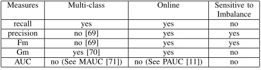
The properties of the above measures are summarized in Table II. They are defined under the two-class context. They cannot be used to evaluate multi-class data directly, except for recall. Their multi-class versions have been devel-oped [69] [70] [71]. The “multi-class” and “online” columns in the table show whether the corresponding measure can be used directly without modification in multi-class and online data scenarios.

TABLE II: Performance evaluation measures for class imbal-ance problems.

Measures Multi-class Online Sensitive to Imbalance

recall yes yes no

precision no [69] yes yes

Fm no [69] yes yes

Gm yes [70] yes no

AUC no (See MAUC [71]) no (See PAUC [11]) no

2) Concept drift: Concept drift is said to occur when the joint probability P(x, y) changes [8] [72] [73]. The key research topics in this area include:

(a)How many types of concept drift are there? Which type is more challenging?

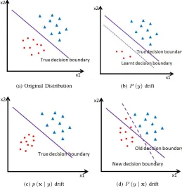
Concept drift can manifest three fundamental forms of changes corresponding to the three major variables in the Bayes’ theorem [74]: 1) a change in prior probability P(y); 2) a change in class-conditional pdf p(x|y); 3) a change in posterior probability P(y|x). The three types of concept drift are illustrated in Figure 2, comparing to the original data distribution shown in Figure 2(a).

Fig. 2(b) shows the P(y) type of concept drift without affecting p(x|y) and P(y|x). The decision boundary re-mains unaffected. The prior probability of the circle class is reduced in this example. Such change can lead to class imbalance. A well-learnt discrimination function may drift away from the true decision boundary, due to the imbalanced class distribution.

Fig. 2(c) shows the p(x|y) type of concept drift without affecting P(y) and P(y|x). The true decision boundary remains unaffected. Elwell and Polikar claimed that this type of drift is the result of an incomplete representation of the true distribution in current data, which simply requires providing supplemental data information to the learning model [75].

(6)

(a) Original Distribution (b)P(y)drift

(c)p(x|y)drift (d)P(y|x)drift

Fig. 2: Illustration of 3 concept drift types.

or partially unsuitable, and the learning model needs to be adapted to the new knowledge.

The posterior distribution change clearly indicates the most fundamental change in the data generating function. This is classified asreal concept drift. The other two types belong to

virtual concept drift [7], which does not change the decision (class) boundaries. In practice, one type of concept drift may appear in combination with other types.

Existing studies primarily focus on the development of drift detection methods and techniques to overcome the real drift. There is a significant lack of research on virtual drift, which can also deteriorate classification performance. As illustrated in Fig. 2(b), even though these types of drift do not affect the true decision boundaries, they can cause a well-learnt decision boundary to become unsuitable. Unfortunately, the current techniques for handling real drift may not be suitable for virtual drift, because they present very different learning difficulties and require different solutions. For instance, the methods for handling real drift often choose to reset and retrain the classifier, in order to forget the old concept and better learn the new concept. This is not an appropriate strategy for data with virtual drift, because the examples from previous time steps may still remain valid and help the current classification in virtual drift cases. It would be more effective and efficient to calibrate the existing classifier than retraining it. Besides, techniques for handling real drift typically rely on feedback about the performance of the classifier, while techniques for handling virtual drift can operate without such feedback [8]. From our point of view, all three types are equally important. Particularly, the two virtual types require more research effort than currently dedicated work by our community. A systematic study of the challenges in each type

will be given in Section IV.

Concept drift has further been characterized by its speed, severity, cyclical nature, etc. A detailed and mutually exclusive categorization can be found in [73]. For example, according to speed, concept drift can be either abrupt, when the generating function is changed suddenly (usually within one time step), or gradual, when the distribution evolves slowly over time. They are the most commonly discussed types in the literature, because the effectiveness of drift detection methods can vary with the drifting speed. While most methods are quite success-ful in detecting abrupt drifts, as future data is no longer related to old data [76], gradual drifts are often more difficult, because the slow change can delay or hide the hint left by the drift. We can see some drift detection methods specifically designed for gradual concept drift, such as Early Drift Detection method (EDDM) [77].

(b)How can we tackle concept drift effectively (state-of-the-art solutions)?

There is a wide range of algorithms for learning in non-stationary environments. Most of them assume and specialize in some specific types of concept drift, although real-world data often contains multiple types. They are commonly cate-gorized into two major groups: active vs. passive approaches, depending on whether an explicit drift detection mechanism is employed. Active approaches (also known as trigger-based approaches) determine whether and when a drift has occurred before taking any actions. They operate based on two mecha-nisms – a change detector aiming to sense the drift accurately and timely, and an adaptation mechanism aiming to maintain the performance of the classifier by reacting to the detected drift. Passive approaches (also known as adaptive classifiers) evolve the classifier continuously without an explicit trigger reporting the drift. A comprehensive review of up-to-date techniques tackling concept drift is given by Ditzler et al. [16]. They further organise these techniques based on their core mechanisms, summarized in Table III. This table will help us to understand how online class imbalance algorithms are designed, which will be introduced in details in Section III. There exist other ways to classify the proposed algorithms, such as Gama et al.’s taxonomy based on the four modules of an adaptive learning system [8], and Webb et al.’s quantitative characterization [78]. This paper adopts the one proposed by Ditzler et al. [16] for its simplicity.

(7)

TABLE III: Categorization of concept drift techniques. See [16] for the full list of techniques under each category.

Active

Step1. Change

Hypothesis tests: assess the validity of a hypothesis by comparing the distributions of two sets of fix-length data sequences.

Change-point methods: identify the change point by analyzing all possible partitions of a fixed data sequence.

detection Sequential hypothesis tests: provide a one-off detection of change or no change, by inspecting incoming examples one by one (sequentially).

Change detection tests: analyze the statistical behavior of streams of data in a fully sequential manner, such as a feature value or classification error. They are either based on a pre-defined threshold or some statistical features representing current data.

Step2. Classifier

Windowing: the classifier is retrained based on a window with up-to-date examples. The window length can be either fixed or adaptive.

Weighting: all received examples are weighted according to time or classification error, which are then used to adaptation update the classifier.

Random Sampling: the examples used to retrain the classifier are randomly chosen based on certain rules. Ensemble: build a new model in the classifier for the new concept.

Passive Single classifier: update a single classifier, such as decision trees, online information network, and extreme learning machine. Ensemble: add, remove or modify the models in an ensemble classifier.

metrics that are more robust to the imbalance degree. More details will be given in Section III. Some other algorithms are specifically designed for data streams coming in batches, such as AUE [82] and the Learn++ family [75]. These algorithms cannot be applied to online cases directly.

(c) How do we evaluate the performance of concept drift detectors and online classifiers?

To fully test the performance of drift detection approaches (especially an active detector), it is necessary to discuss both data with artificial concept drifts and real-world data with unknown drifts. Using data with artificial concept drifts allows us to easily manipulate the type and timing of concept drifts, so as to obtain an in-depth understanding of the performance of approaches under various conditions. Testing on data from real-world problems helps us to understand their effectiveness from the practical point of view, but the information about when and how concept drift occurs is unknown in most cases. The following aspects are usually considered to assess the accuracy of active drift detectors. Their measurement is based on data with artificial concept drifts where drifts are known.

• True detection rate: the possibility of detecting the true concept drift. It shows the accuracy of the detection approach.

• False alarm rate: the possibility of reporting a concept drift that does not exist (false-positive rate). It character-izes the costs and reliability of the detection approach.

• Delay of detection: an estimate of how many time steps are required on average to detect a drift after the actual occurrence. It reflects how much time would be taken before the drift is detected.

Wang and Abraham [10] use a histogram to visualize the distribution of detection points from the drift detection approach over multiple runs. It reflects all the three aspects above in one plot. It is worth nothing that there are trade-offs between these measures. For example, an approach with a high true detection rate may produce a high false alarm rate. A very recent algorithm, Hierarchical Change-Detection Tests (HCDTs), was proposed to explicitly deal with the trade-off [83].

After the performance of drift detection approaches is better understood, we need to quantify the effect of those detections on the performance of predictive models. All the performance

metrics introduced in the previous section of “class imbalance” can be used. The key question here is how to calculate them in the streaming settings with evolving data. The performance of the classifier may get better or worse every now and then. There are two common ways to depict such performance over time – holdout and prequential evaluation [8].

Holdout evaluation is mostly used when the testing data set (holdout set) is available in advance. At each time step or every few time steps, the performance measures are calculated based on the valid testing set, which must represent the same data concept as the training data at that moment. However, this is a very rigorous requirement for data from real-world applications.

In prequential evaluation, data received at each time step is used for testing before it is used for training. From this, the performance measures can be incrementally updated for evaluation and comparison. This strategy does not require a holdout set, and the model is always tested on unseen data.

When the data stream is stationary, the prequential perfor-mance measures can be computed based on the accumulated sum of a loss function from the beginning of the training. However, if the data stream is evolving, the accumulated measure can mask the fluctuation in performance and the adaptation ability of the classifier. For example, consider that an online classifier correctly predicts 90 out of 100 examples received so far (90% accuracy on data with the original concept). Then, an abrupt concept drift occurs at time step 101, which makes the classifier only correctly predict 3 out of 10 examples from the new concept (30% accuracy on data with the new concept). If we use the accumulated measure based on all the historical data, the overall accuracy will be 93/110, which seems to be high but does not reflect the true performance on the new data concept. This problem can be solved by using a sliding window or a time-based fading factor that weigh observations [84].

III. OVERCOMINGCLASSIMBALANCE ANDCONCEPT

DRIFTSIMULTANEOUSLY

(8)

the drift detection algorithms based on the traditional clas-sification error may be sensitive to imbalanced degree and become less effective; the class imbalance techniques need to be adaptive to changing P(y), otherwise the class receiving the preferential treatment may not be the correct minority class at the current moment. Therefore, their mutual effect should be considered during the algorithm design.

A. Illustrative Applications

The combined problems of concept drift and class imbal-ance have been found in many real-world applications. Three examples are given here, to help us understand each type of concept drift.

1) Environment monitoring with P(y) drift: Environment monitoring systems usually consist of various sensors gener-ating streaming data in high speed. Real-time prediction is required. For example, a smart building has sensors deployed to monitor hazardous events. Any sensor fault can cause catastrophic failures. Machine learning algorithms can be used to build models based on the sensor information, aiming to predict faults in sensors accurately and timely [3]. First, the data is characterized by class imbalance, because obtaining a fault in such systems can be very expensive. Examples repre-senting faults are the minority. Second, the number of faults varies with the faulty condition. If the damage gets worse over time, the faults will occur more and more frequently. It implies a prior probability change, a type of virtual concept drift.

2) Spam filtering with p(x|y) drift: Spam filtering is a typical classification problem involving class imbalance and concept drift [85]. First of all, the spam class is the minority and suffers from a higher misclassification cost. Second, the spammers are actively working on how to break through the filter. It means that the adversary actions are adaptive. For example, one of the spamming behaviours is to change email content and presentation in disguise, implying a possible class-conditional pdf (p(x|y)) change [8].

3) Social media analysis with P(y|x) drift: In social media (e.g. twitter, facebook), consider the example where a company would like to make relevant product recommenda-tions to people who have shown some type of interest in their tweets. Machine learning algorithms can be used to discover who is interested in the product based on the tweets [86]. The number of users who have shown the interest is always very small. So, this is a minority class. Meanwhile, users’ interest changes from time to time. Users may lose their interest in the current trendy product very quickly, causing posterior probability (P(y|x)) changes.

Although the above examples are associated with only one type of concept drift, different types often coexist in real-world problems, which are hard to know in advance. For the example of spam filtering, which email belongs to spam also depends on users’ interpretation. Users may re-label a particular category of normal emails as spam, which indicates a posterior probability change.

B. Approaches to Tackling Both Class Imbalance and Concept Drift

Some research efforts have been made to address the joint problem of concept drift and class imbalance, due to the rising need from practical problems [87] [1]. Uncorrelated Bagging is one of the earliest algorithms, which builds an ensemble of classifiers trained on a more balanced set of data through resampling and overcomes concept drift passively by weighing the base classifier based on their discrimina-tive power [88] [89] [90]. Selecdiscrimina-tively recursive approaches SERA [91] and REA [92] use similar ideas to Uncorrelated Bagging of building an ensemble of weighted classifiers, but with a “smarter” oversampling technique. Learn++.CDS and Learn++.NIE are more recent algorithms, which tackle class imbalance through the oversampling technique SMOTE [33] or a sub-ensemble technique, and overcome concept drift through a dynamic weighting strategy [93]. HUWRS.IP [94] improves HUWRS [95] to deal with imbalanced data streams by introducing an instance propagation scheme based on a Na¨ıve Bayes classifier, and using Hellinger distance as a weighting measure for concept drift detection. The Hellinger weight for drift detection is calculated as the average of the minority-class and majority-class Hellinger distance between the two feature distributions. It guarantees equal weight to the Hellinger distance between the minority-class and majority-class distributions. The instance propagation scheme selects old minority-class examples that are relevant to the current data concept. It avoids the problem of using misleading ex-amples from the old data concept. However, relevant exex-amples may not exist in some rapid drifting cases. So, Hellinger Dis-tance Decision Tree (HDDT) was proposed to use Hellinger distance as the decision tree splitting criteria that is imbalance-insensitive [96]. All these approaches belong to chunk-based learning algorithms. Their core techniques work when a batch of data is received at each time step, i.e., they are unsuitable for online processing. Developing a true online algorithm for concept drift is very challenging because of the difficulties in measuring minority-class statistics using only one example at a time [16].

(9)

TABLE IV: Online approaches to tackling concept drift and class imbalance, and their properties.

Approaches Category? Class Access to Additional Multi- Drift type? imbalance? old data? data? class?

DDM-OCI [9] Active (change detection test + windowing) No No No No P(y|x) LFR [10] Active (change detection test + windowing) No No No No P(y|x) PAUC-PH [11] Active (change detection test + windowing) No Yes No No P(y|x) RLSACP [14]/ONN [98] Passive (single classifier) Yes Yes No No all 3 types

ESOS-ELM [15] Passive+Active (ensemble) Yes No Yes No p(x|y),P(y|x)

OOB/UOB using CID [13] Active (weighting) Yes No No No P(y)

indicator in Page-Hinkley (PH) test [97]. However, it needs access to historical data. DDM-OCI, LFR and PAUC-based PH test are active drift detectors designed for imbalanced data streams, and are independent of classification algorithms. They aim at concept drift with classification boundary changes by default. Therefore, if a concept drift is reported, they will reset and retrain the online model. Although these drift detectors are designed for imbalanced data, they themselves do not involve any class imbalance techniques, such as resampling, to adjust the decision boundary of the online model. It is still unclear how they perform when working with class imbalance techniques.

Besides the above active approaches, the perceptron-based algorithms RLSACP [14], ONN [98] and ESOS-ELM [15] adapt the classification model to non-stationary environments passively, and involve mechanisms to overcome class imbal-ance. RLSACP and ONN are single-model approaches with the same general idea. Their error function for updating the perceptron weights is modified, including a forgetting function for model adaptation and an error weighting strategy as the class imbalance treatment. The forgetting function has a pre-defined form, allowing the old data concept to be forgotten gradually. The error weights in RLSACP are incrementally updated based either on the classification performance or the imbalance rate from recently received data. It was shown that weight updating based on the imbalance rate leads to better performance.

ESOS-ELM is an ensemble approach, maintaining a set of online sequential extreme learning machines (OS-ELM) [99]. For tackling class imbalance, resampling is applied in a way that each OS-ELM is trained with approximately equal number of minority- and majority-class examples. For tackling concept drift, voting weights of base classifiers are updated according to their performance G-mean on a separate validation data set from the same environment as the current training data. In addition to the passive drift detection technique, ESOS-ELM includes an independent module – ELM-store, to handle re-curring concept drift. ELM-store maintains a pool of weighted extreme learning machines (WELM) [66] to retain old infor-mation. It adopts a threshold-based technique and hypothesis testing to detect abrupt and gradual concept drift actively. If a concept drift is reported, a new WELM will be built and kept in ELM-store. If any stored model performs better than the current OS-ELM ensemble, indicating a possible recurring concept, it will be introduced in the ensemble. ESOS-ELM assumes the imbalance rate is known in advance and fixed. It needs a separate data set for initializing OS-ELMs and WELMs, which must include examples from all classes. It

is also necessary to have validation data sets reflecting every data concept for concept drift detection, which can be a quite restrictive requirement for real-world data.

With a different goal of concept drift detection from the above, a class imbalance detection (CID) approach was pro-posed, aiming at P(y) changes [20]. It reports the current imbalance status and provides information of which classes belong to the minority and which classes belong to the majority. Particularly, a key indicator is the real-time class size w(t)_k , the percentage of class ck at time step t. When a

new examplext arrives,w

(t)

k is incrementally updated by the

following equation [20]:

w(t)_k =θw_k(t−1)+ (1−θ) [(xt, ck)],(k= 1, . . . , N) (5)

where [(xt, ck)] = 1 if the true class label of xt is ck,

and 0 otherwise. θ (0< θ <1) is a pre-defined time decay (forgetting) factor, which reduces the contribution of older data to the calculation of class sizes along with time. It is independent of learning algorithms, so it can be used with any type of online classifiers. For example, it has been used in OOB and UOB [13] for deciding the resampling rate adap-tively and overcoming class imbalance effecadap-tively over time. OOB and UOB integrate oversampling and undersampling re-spectively into ensemble algorithm Online Bagging (OB) [65]. Oversampling and undersampling are one of the simplest and most effective techniques of tackling class imbalance [31].

The properties of the above online approaches are summa-rized in Table IV, answering the following six questions in order:

• How do they handle concept drift (the type based on the

categorization in Table III)?

• Do they involve any class imbalance technique to improve

the predictive performance of online models, in addition to concept drift detection?

• Do they need access to previously received data?

• Do they need additional data sets for initialisation or validation?

• Can they handle data streams with more than two classes (multi-class data)?

• Which type of concept drift can it deal with?

IV. PERFORMANCEANALYSIS

(10)

what are the difficulties in detecting each type of concept drift? Little work has given separate discussions on the three fundamental types of concept drift, especially the P(y)drift. It is important to understand their differences, so that the most suitable approaches can be used for the best performance.

2) Among existing approaches designed for imbalanced data streams with concept drift, which approach is better and when?Although a few approaches have been proposed for the purpose of overcoming concept drift and class imbalance, it is still unclear how well they perform for each type of concept drift.3) Whether and how do class imbalance techniques affect concept drift detection and online prediction? No study has looked into the mutual effect of applying class imbalance techniques and concept drift detection methods. Understanding the role of class imbalance techniques will help us to develop more effective concept drift detection methods for imbalanced data.

A. Data Sets

For an accurate analysis and comparable results, we choose two most commonly used artificial data generators, SINE1 [80] and SEA [100], to produce imbalanced data streams containing three simulated types of concept drift. In SINE1, each gener-ated point has two attributes(x1, x2), uniformly distributed in

[0,1]. The concept is decided by where the point is located (above the sin function or not). In SEA, each sample has three attributesx1,x2 andx3 with values between 0 and 10.

Only the first two attributes are relevant. The class label is determined by a threshold.

This is one of the very few studies that individually discuss P(y),p(x|y)andP(y|x)types of concept drift in depth. In addition, each generator produces two data streams with a different drifting speed – abrupt and gradual drifts. The drifting speed is defined as the inverse of the time taken for a new concept to completely replace the old one [73]. According to speed, drifts can be either abrupt, when the generating function is changed completely in only one time step, or gradual, otherwise. The data streams with a gradual concept drift are denoted by ‘g’ in the following experiment, i.e. SINE1g [77] and SEAg. Every data stream has 3000 time steps, with one concept drift starting at time step 1501. The new concept in SINE1 and SEA fully takes over the data stream from time step 1501; the concept drift in SINE1g and SEAg takes 500 time steps to complete, which means that the new concept fully replaces the old one from time step 2001. The detailed settings for generating each type of concept drift are included in the individual subsections.

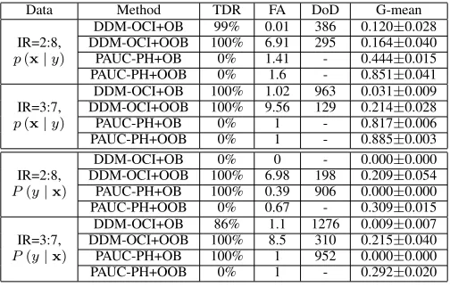
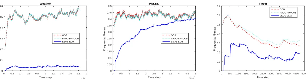
After the detailed analysis of the three types of concept drift, three real-world data sets are included in our experiment with unknown concept drift, which are PAKDD 2009 credit card data (PAKDD) [101], Weather data [76] and UDI Tweet-erCrawl data [102]. Data in PAKDD are collected from the private label credit card operation of a Brazilian retail chain. The task of this problem is to identify whether the client has a good or bad credit. The “bad” credit is the minority class, taking 19.75% of the provided modelling data. Because the data have been collected from a time interval in the past,

gradual market change occurs. The Weather data set aims to predict whether rain precipitation was observed on each day, with inherent seasonal changes. The class of “rain” is the minority, taking 31% of the data set. The original Tweet data include 50 million tweets posted mainly from 2008 to 2011. The task is to predict the tweet topic. We choose a time interval, containing 8774 examples and covering seven tweet topics [103]. Then, we further reduce it to 2-class data by using only two out of seven topics for our experiment. These real-world data will help us to understand the effectiveness of existing concept drift and class imbalance approaches in practical scenarios, which usually have more complex data distributions and concept drift.

B. Experimental and Evaluation Settings

The approaches listed in Table IV, which are explicitly designed for the combined problem of class imbalance and concept drift, are discussed in our experiment. For the three active drift detection methods – DDM-OCI, LFR and PAUC-PH, they need to work with online learning algorithms for classification. We choose two approaches to build the online model, the traditional Online Bagging (abbr. OB) [65] and OOB with CID [13], to build the online model. Because OOB applies oversampling to overcome class imbalance and OB does not, it can help us to observe the role of class imbalance techniques (oversampling in our experiment) in concept drift detection. UOB is not chosen, for the consideration that undersampling may cause unstable performance which may indirectly affect our observation [13]. Between RLSACP and ONN, due to their similarity and the more theoretical support in RLSACP, only RLSACP is included in our experiment.

Considering RLSACP and ESOS-ELM are perceptron-based methods, we use the Multilayer Perceptron (MLP) classifier as the base learner of OB and OOB. The number of neurons in the hidden layer of MLPs is set to the average of the number of attributes and classes in data, which is also the number of perceptrons in RLSACP and in the base learner of ESOS-ELM. All ensemble methods maintain 15 base learners. For ESOS-ELM, we disable the “ELM-Store”, which is designed for recurring concept drift; we allow that its ensemble size can grow to 20. In addition, ESOS-ELM requires an initialisation data set to initialize ELMs, and validation data sets to adjust misclassification costs. When dealing with artificial data, we use the first 100 examples to initialize ESOS-ELM, and generate a separate validation data set for each concept stage. We track the performance of all the methods from time step 101.

In summary, ten algorithms join the comparison from Table IV: OB, OOB, DDM-OCI+OB/OOB, PAUC-PH+OB/OOB, LFR+OB/OOB, RLSACP and ESOS-ELM. OB is the baseline without involving any class imbalance and concept drift techniques.

(11)

TABLE V: Artificial data streams withP(y)concept drift.

ID Data Speed Class +1 Class -1

Concept OldP(y) NewP(y) Concept OldP(y) NewP(y) 1 SINE1 Abrupt

Points belowx2= sin (x1) 0.1 0.9 Points above or onx2= sin (x1) 0.9 0.1

2 SINE1g Gradual

3 SEA Abrupt _x

1+x2≤7 0.5 0.1 x1+x2>7 0.5 0.9

4 SEAg Gradual

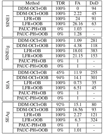
comparison, because they are insensitive to imbalance rates. When discussing the generated artificial data sets with ground truth known, we also compare the true detection rate (abbr. TDR), total number of false alarms (abbr. FA) and delay of detection (abbr. DoD) (as defined in Section II) among methods using any of the three active drift detectors (i.e. DDM-OCI, LFR and PAUC-PH). The calculation of TDR, FA and DoD is the same for both of the abrupt and the gradual drifting cases, based on the following understanding: before a real concept drift occurs (before time step 1500 in our cases), all the reported alarms are considered as false alarms; after a real concept drift starts (after time step 1500 in our cases), the first detection is seen as the true drift detection; after that and before the next new real concept drift, the consequent detections are considered as false alarms.

Furthermore, because we are particularly interested in how the learner performs on the new data concept in the artificial data sets, we calculate the average recall and G-mean over all the time steps after the concept drift completely ends (time step 1500 for the abrupt drifting cases and time step 2000 for the gradual drifting cases). It is worth noting that the recall and G-mean values are reset to 0 when the drift starts and ends for an accurate analysis. We use the Wilcoxon Sign Rank test at the confidence level of 95% as our significance test in this paper.

C. Comparative Study on Artificial Data

C.1. P(y)Concept Drift

This section focuses on the P(y) type of concept drift, withoutp(x|y)andP(y|x)changes. Data streams SINE1 and SINE1g have a severe class imbalance change, in which the minority (majority) class during the first half of data streams becomes the majority (minority) during the latter half. SEA and SEAg have a less severe change, in which the data stream presented to be balanced during the first half becomes imbalanced during the latter half. P(y) is changed linearly during the concept transition period (time step 1501 to time step 2000) in the gradual drifting cases. The concrete setting for each data stream is summarized in Table V.

Table VI compares the detection performance of the three active concept drift detectors, in terms of TDR, FA and DoD. We can see that DDM-OCI and LFR are sensitive to class imbalance changes in data. They present very high true detection rate; especially, LFR has 100% TDR in all cases regardless of whether resampling is used to tackle class imbalance. PAUC-PH does not report any concept drift, showing 0% TDR in all cases. This is because DDM-OCI and LFR use time-decayed metrics as the indicator of concept drift, which have higher sensitivity to performance change in general than the prequential AUC used by PAUC-PH. LFR

shows even higher TDR than DDM-OCI, because it tracks four rates in the confusion matrix instead of one. For the same reason, DDM-OCI and LFR have a higher chance of issuing false alarms than PAUC-PH. For DDM-OCI, oversampling in OOB increases the probability of reporting a concept drift by observing TDR in SEA and SEAg, compared to OB. This is because more examples are used for training in OOB, which improves the performance on the minority class for concept drift detection.

TABLE VI: Performance of the 3 active concept drift detectors on artificial data withP(y)changes: TDR, FA and DoD. The ‘-’ symbol indicates that no concept drift is detected.

Method TDR FA DoD

SINE1

DDM-OCI+OB 100% 0 94 DDM-OCI+OOB 100% 2.22 45 LFR+OB 100% 24 91 LFR+OOB 100% 26.16 63 PAUC-PH+OB 0% 1.03 -PAUC-PH+OOB 0% 1.28

-SINE1g

DDM-OCI+OB 100% 1.09 281 DDM-OCI+OOB 100% 4.38 118 LFR+OB 100% 18.01 383 LFR+OOB 100% 21.15 153

PAUC-PH+OB 0% 1

-PAUC-PH+OOB 0% 1

-SEA

PAUC-PH+OB 0% 1

-PAUC-PH+OOB 0% 1

-SEAg

PAUC-PH+OB 0% 1

-PAUC-PH+OOB 0% 1.01

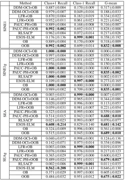
-Table VII compares recall and G-mean of all models over the new data concept, i.e. performance over time steps 1501-3000 for data streams with an abrupt change and performance over time steps 2001-3000 for data streams with a gradual change, showing whether and how well the drift detector can help with learning after concept drift is completed. In SINE1 and SINE1g, the negative class presents to be the minority after the change; in SEA and SEAg, the positive class presents to be the minority after the change.

(12)

TABLE VII: Performance of online learners on artificial data withP(y)changes: means and standard deviations of average recall of each class and average G-mean over the new data concept. The significantly best values among all methods are shown in bold italics.

Method Class+1 Recall Class-1 Recall G-mean

SINE1

DDM-OCI+OB 0.887±0.004 0.170±0.009 0.317±0.009 DDM-OCI+OOB 0.979±0.007 0.049±0.016 0.188±0.033 LFR+OB 0.870±0.004 0.183±0.019 0.334±0.022 LFR+OOB 0.952±0.011 0.061±0.023 0.221±0.042 PAUC-PH+OB 0.889±0.004 0.168±0.008 0.316±0.007 PAUC-PH+OOB 0.992±0.002 0.692±0.013 0.828±0.008 RLSACP 0.962±0.004 0.072±0.014 0.217±0.026 ESOS-ELM 0.176±0.136 0.999±0.001 0.358±0.192 OB 0.889±0.004 0.170±0.009 0.318±0.009 OOB 0.992±0.002 0.699±0.014 0.832±0.008

SINE1g

SEA

SEAg

It also explains that OOB and OOB using PAUC-PH have very close performance. None of the other OB and OOB models show competitive recall and G-mean. Especially for those using DDM-OCI and LFR, their G-mean is significantly lower than PAUC-PH with OOB models, due to their high FA. The high number of false alarms causes too much resetting and performance loss. OOB can increase the chance of producing a false alarm, based on the observation that it led to a higher FA than OB models, because more minority-class examples join the training. This explains why G-mean from DDM-OCI and LFR is even lower in OOB models than in OB models, for the case of SINE1.

Therefore, we conclude that, forP(y)type of concept drift, it is not necessary to apply any drift detection techniques that are not specifically designed for class imbalance changes; the use of these drift detectors could be even detrimental to the predictive performance due to false alarms and performance resetting; the adaptive resampling in OOB is sufficient to deal with the change and maintain the predictive performance; when using OOB with other active concept drift detectors, the number of false alarms and performance resetting need to be

carefully considered.

C.2.p(x|y)Concept Drift

The data streams in this section only involvep(x|y)type of concept drift, without P(y) and P(y|x) changes. The class imbalance ratio is fixed to 1:9 and we let the positive class be the minority, so that the data stream is constantly imbalanced. The concept drift in each data stream is controlled byp(x)of the negative class, as shown in Table VIII.P(x1)

is changed linearly during the concept transition period in the gradual drifting cases.

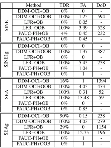
Table IX compares the detection performance of the three active concept drift detectors. Similar to our previous results, DDM-OCI and LFR are more sensitive to P(x|y)changes than PAUC-PH. When DDM-OCI and LFR work with OOB, their TDR shows 100%; and LFR has higher FA and shorter DOD than DDM-OCI, due to more indicators it monitors. PAUC-PH shows 0% TDR in most cases of working with both OB and OOB. Different from P(y) changes, when DDM-OCI and LFR work with OB, their TDR is rather low, which suggests that their sensitivity is dependent on the class imbalance techniques. To explain this, we observe OB’s recall of each class over time. Unlike the cases with class imbalance changes, where it is possible for the minority-class examples to become more frequent, the data streams generated in this section have a fixed minority class with a constantly small prior probability. The minority-class recall remains low (e.g. 0 in SINE1 and SINE1g cases) due to the imbalanced distribution. These detectors cannot detect any concept drift, because the classification performance they monitored does not change significantly. In other words, the classification dif-ficulty indirectly affects the detection sensitivity of DDM-OCI and LFR. When oversampling is applied, which introduces more training examples for the minority class, the performance metrics (G-mean, recall and precision) monitored by DDM-OCI and LFR can be substantially improved. It also increases the possibility of reporting a concept drift. This explains the low detection rate of DDM-OCI and LFR when working with OB and their high detection rate when working with OOB.

(13)

TABLE VIII: Artificial data streams withp(x|y)concept drift.

ID Data Speed Class +1 Class -1

Old concept New concept Old concept New concept

1 SINE1 Abrupt Points below Points below Points above or onx2= sin (x1) Points above or onx2= sin (x1)

2 SINE1g Gradual x2= sin (x1) x2= sin (x1) andP(x1<0.5) = 0.9 andP(x1<0.5) = 0.1

3 SEA Abrupt _x

1+x2≤7 x1+x2≤7 x1+x2>7 x1+x2>7

4 SEAg Gradual andP(x1<5) = 0.9 andP(x1<5) = 0.1

TABLE IX: Performance of the 3 active concept drift detectors on artificial data with p(x|y)changes: TDR, FA and DoD. The ‘-’ symbol indicates that no concept drift is detected.

Method TDR FA DoD

SINE1

DDM-OCI+OB 0% 0

-DDM-OCI+OOB 100% 1.25 594

LFR+OB 0% 0.05

-LFR+OOB 100% 3.99 528 PAUC-PH+OB 4% 0.45 232 PAUC-PH+OOB 0% 0.45

-SINE1g

DDM-OCI+OB 0% 0

-DDM-OCI+OOB 100% 1.37 387

LFR+OB 0% 0

-LFR+OOB 100% 5.45 258 PAUC-PH+OB 0% 1.04

-PAUC-PH+OOB 0% 1

-SEA

DDM-OCI+OB 16% 1 1394 DDM-OCI+OOB 100% 4.03 473

LFR+OB 100% 0.31 52 LFR+OOB 100% 13.48 59

PAUC-PH+OB 0% 0

-PAUC-PH+OOB 0% 0.85

-SEAg

DDM-OCI+OB 90% 0.15 238 DDM-OCI+OOB 100% 4.03 279

LFR+OB 29% 0 1154

LFR+OOB 100% 12.75 196

PAUC-PH+OB 0% 1

-PAUC-PH+OOB 0% 1

-achieves the best performance. Besides, while the adopted class imbalance technique can improve the final prediction, it can also improve the performance of active concept drift detection methods, depending on their working mechanism.

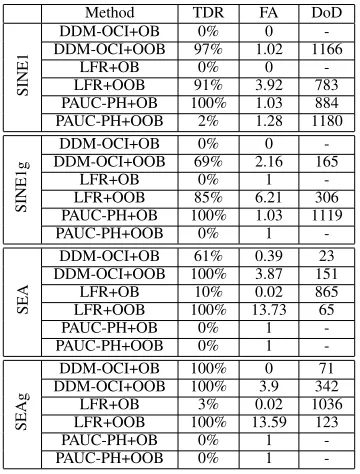
C.3. P(y|x)Concept Drift

The data streams in this section only involve P(y|x)

type of concept drift, without P(y) and p(x|y) changes. Following the settings in Section IV-C.2, we fix the class imbalance ratio to 1:9 and let the positive class be the minority, so that the data stream is constantly imbalanced. As shown in Table XI, the data distribution in SINE1 and SINE1g involves a concept swap, and this change occurs probabilistically in SINE1g; the data distribution in SEA and SEAg has a concept threshold moving, and this change occurs continuously in SEAg. The change in SEA and SEAg is less severe than the change in SINE1 and SINE1g, because some of the examples from the old concept are still valid under the new concept after the threshold moves completely. The concept drift discussed in this section belongs to the real concept drift category, which affects the classification boundary and is expected to be captured by all concept drift detectors.

According to Table XII, we can see that DDM-OCI and LFR have difficulty in detecting the concept drift when working with OB, because of the poor recall and G-mean produced by OB, which is also observed and explained in Section IV-C.2.

TABLE X: Performance of online learners on artificial data with p(x|y) changes: means and standard deviations of average recall of each class and average G-mean over the new data concept. The significantly best values among all methods are shown in bold italics.

Method Class+1 Recall Class-1 Recall G-mean

SINE1

SINE1g

SEA

SEAg