http://www.sciencepublishinggroup.com/j/acm doi: 10.11648/j.acm.20190805.11
ISSN: 2328-5605 (Print); ISSN: 2328-5613 (Online)
On Optimal Parameter Not Only for the SOR Method
Stanislaw Marian Grzegorski
Institute of Computer Science, Lublin University of Technology, Nadbystrzycka, Lublin, Poland
Email address:
To cite this article:
Stanislaw Marian Grzegorski. On Optimal Parameter Not Only for the SOR Method. Applied and Computational Mathematics.
Vol. 8, No. 5, 2019, pp. 82-87. doi: 10.11648/j.acm.20190805.11
Received: October 15, 2019; Accepted: November 18, 2019; Published: November 22, 2019
Abstract:
The Jacobi, Gauss-Seidel and SOR methods belong to the class of simple iterative methods for linear systems. Because of the parameter ω, the SOR method is more effective than the Gauss-Seidel method. Here, a new approach to the simple iterative methods is proposed. A new parameter q can be introduced to every simple iterative method. Then, if a matrix of a system is positive definite and the parameter q is sufficiently large, the method is convergent. The original Jacobi method is convergent only if the matrix is diagonally dominated, while the Jacobi method with the parameter q is convergent for every positive definite matrix. The optimality criterion for the choice of the parameter q is given, and thus, interesting results for the Jacobi, Richardson and Gauss-Seidel methods are obtained. The Gauss-Seidel method with the parameter q, in a sense, is equivalent to the SOR method. From the formula for the optimal value of qresults the formula for optimal value of ω. Up to present, this formula was known only in special cases. Practical useful approximate formula for optimal value ω is also given. The influence of the parameter q on the speed of convergence of the simple iterative methods is shown in a numerical example. Numerical experiments confirm: for very large scale systems the speed of convergence of the SOR method with optimal or approximate parameter ω is near the same (in some cases better) as the speed of convergence of the conjugate gradients method.Keywords:
Iterative Methods for Linear Systems, Optimal Parameter for SOR Method, Positive Definite Matrices1. Introduction
The solution of linear systems is a fundamental problem in numerical analysis, especially, if the system has a very large scale. Such systems appear while solving partial differential equations, nonlinear systems or optimization problems. The literature in this area is very rich, for example, Koutis et al. [1] present a very interesting fast algorithm for solving linear systems using the techniques of graph theory, but their method can be used only for symmetric diagonally dominant matrices. In solving the linear systems, preconditions play a very important role. Because of preconditions, the algorithm proposed by Boman and Scott [2] for elliptic finite element systems is near-linear. Hogg and Scott [3] apply a direct method to obtain an approximate solution and then use an iterative method to improve its accuracy. Here, we return to the classical simple iterative methods, such as the following: the Jacobi method, the Richardson method, the Gauss-Seidel method and the Successive Over-Relaxation (SOR) method. The theoretical basis of the simple iterative methods can be found in [4-7]. Broyden [8] gives the theorem about
convergence of the SOR method. There are many results concerning the optimal parameter for the SOR method. Up to now, the formula for optimal parameter for the SOR method is known only in special cases. For example, in the papers [6, 9, 10] you can find exact formula for optimal parameter for some discretization of Poisson equation. Here, we give such formula for every positive definite and symmetric matrix. In papers [11-13] the authors use an approximate value of the parameter . Nevanlinna [14] explains why the SOR and conjugate gradients methods are essentially equally fast for discretized Laplacians. Additionally, Woźniakowski [15] has proved that under some assumptions Jacobi, Gauss-Seidel and SOR methods are numericly stable.
Let us consider the linear system
(1) where , , , and is a positive definite matrix. Let be divided into two parts, i.e. , where is a nonsingular matrix and the linear system
follows:
0
− , = 0,1,2, … (2)
Let = + ! + ", where ! is the diagonal matrix and
, " are lower and upper triangular matrices, respectively. If
= !, we obtain the Jacobi method; if = + ! we obtain the Gauss-Seidel method; if = +#$, (0,2), we obtain the SOR method. Here, we introduce a parameter % to the formula (2) in the following way:
( + %&) = − ( − %&) ,
where & is the unit matrix. The simple iterative method with the parameter % is defined as:
= 0
= ( + %&) ( − ( −%&) ), = 0,1,2, … (3)
In the analysis of the convergence, the main role plays the matrix
' = ( + %&) ( − %&) (4) or, more precisely, the spectral radius ((') of the matrix '. A sufficient condition for the convergence is ((') < 1. We can consider the following cases:
= 0. Then the sequence (3) is equivalent to
* = −+= 0
% , = 0,1,2, …
where the residual + = − . In this case we have the Richardson method. If % =,-,./,
--.,-, we then have the minimum
residual (mr) method;
b. = !. In this case we obtain the Jacobi method with the parameter % and, for sufficiently large %, the method is convergent not only for a diagonally dominated, but also for every positive definite matrix;
c. = + !. If % is appropriately chosen, then the effectiveness of the Gauss-Seidel method with % is equivalent to the SOR method;
d. is a block-diagonal matrix; e. is a tri-diagonal matrix.
Why is % important in the simple iterative methods? For a sufficiently large %, the matrix + %& is positive definite and even diagonally dominated. In addition, the conditional number
κ( + %&) =00123(/) 4
156(/) 4 < 7( )
for
% > 0
and
lim
4→=7( + %&) = 1.
The expression >(/)>(/) plays an important role in the analysis of the speed of convergence of some of the iterative methods. In Section 2, one can find the theorem regarding the convergence and speed of convergence of the sequence (3). The optimality criterion for the choice of the parameter % is given. In Section 3, the residual method with % is analyzed and the minimal spectral radius is calculated. The results concerning the Gauss-Seidel and SOR methods can be found in Section 4, and formulas for the optimal values of % and are given. In Section 5, the results of some of the numerical experiments are presented. This Section shows how the number of iterations depends on the parameter %. Additionally, a comparison of the speed of convergence for some of the iterative methods is made.
2. Convergence of the Method
We take under consideration the system (1), where is a positive definite matrix. The sequence ? @ may be written as
= 0,
= − ' , (5)
where = ( + %&) and ' is defined by (4). If A denotes the solution of the system (1), then A = −
' A. Subtracting the last equation from (5), we obtain
− A = −'( − A) (6) The sufficient condition for the convergence of the sequence ? @ has the form ((') < 1. Let an eigenpair
(B(%), ), where B(%) C, C for the matrix ' be given. Then
( − %&) = B(%)( + %&) , ∗ = 1,
where ∗ denotes transposition and complex conjugate of the vector . This equation implies the formula
B(%) = ∗/E 4 ∗/F 4=
∗/
∗/F 4− 1 (7)
and lim4→=B(%) = −1. Next, the theorem about regarding convergence of the sequence (3) will be proved.
Theorem 1. Let be a positive definite matrix. Then there exists % such that for % > %
((') < 1 and ((') ≥ max JK,K,-LFK
-K ,
K-LF -K K- -MFKN for = 1,2, …, (8) where + = − and K K = O .
Proof. Let us denote ∗ = P + QR and ∗ = S + TR, where R = √−1 and P, Q, S, T . Then
B(%) =Y 4 ZXV 4 WX,
and
Because ∗ ∗ ∗ > 0 for ≠ 0, we have
T = −Q and P + S > 0. The inequality |B(%)| < 1 is equivalent to
|S − %| < |P + %| (10)
Let %′ = (S − P). Then P + % > 0 and |S − %| < P + % are satisfied for % > %^. Let us define
% = maxK K_ `a6
? b( ∗ − ∗ )@ (11)
Then ((') < 1 for % > % . Subtracting (6) for − 1 from (6) for , we obtain
− = −'( − )
and
((') ≥K -LF -K
K - -MFK (12)
Let A be the solution of system (1). Then,
+ = − − ( A − ) = ( − A) (13) Because − A = −'( − A), we have
+ = ( − A) = − '( − A) = − ' ( − A) = − ' + .
which implies
K+ K ≤ ((')K+ K (14) This result concludes the proof of Theorem 1.
Remark 1. If is a negative definite matrix, then there exists % such that ((') < 1 for % < % .
Remark 2. If % > (( ), then b?B(%)@ (−1,0). This result means that % should be chosen from the interval
(% , % ), where % is defined in (11) and % = K K=. Remark 3. The function
d(%) = |B(%)| =(S − %) + Q(P + %) + Q
is a unimodal function on the interval (% , ∞), and d(%) reaches its minimum when % = S. This result concerns only one eigenvalue. If we want to choose the optimal % for the sequence ? @, we then must apply the definition B(%) and the following equation
− minK K_ b?B(%)@ = maxK K_ b?B(%)@. (15)
Using (7) and (15) we define the optimality criterion as
minK K_ ./
./F 4= 2 − maxK K_ ./
./F 4 (16)
and then
((') = 1 − minK K_ ./.F/ 4= maxK K_ ./
./F 4− 1. (17)
3. The Richardson Method
Let = 0. Then ' =4( − %&) =/4− & and
λ(') = .4/ − 1, O = 1.
The relation λ(') (−1,1) implies 0 < O < 2%. Thus, if is a positive definite matrix and % > Bgh ( ), then
((') < 1 and the sequence ? @ is convergent to the solution of the system (1). The optimal % should satisfy equation (16)
min K K_
O
% = 2 − maxK K_ O
% ,
and this means
BgX ( ) = 2% − Bgh ( ).
Lastly,
%ijk = lBgX ( ) + Bgh ( )m (18)
and then
((') = maxK K_ n%O
ijk − 1n = 1 − BgX ( )/%ijk =0123(/) 0156(/)
0123(/) 0156(/)= >(/)
>(/) (19)
If we assume XX = p for R = 1,2, … , , then the Jacobi method with parameter % is equivalent to the Richardson method, and for both methods we get the same results.
4. The Gauss-Seidel Method with the
Parameter q
Let be expressed as the sum of three matrices
= + ! + " (20) where D is a diagonal matrix and , " are lower and upper triangular matrices, respectively. The Gauss-Seidel (GS) method is defined by
= ( + !) ( − " ), = 0,1,2, … (21) The successive over-relaxation (SOR) method is also known as the extrapolated Gauss-Seidel method. In this case
= q +1!r sq1! − ! − "r + t,
class of matrices is given in [4]. In contrast, the properties of the Gauss-Seidel method with the parameter % can be analyzed easily, and it is possible to calculate the optimal value % and the spectral radius for '.
Let be a symmetric and positive definite matrix. Then the Gauss-Seidel method with the parameter % has the form
= − ' (23) where = ( + ! + %&) , ' = ( + ! + %&) ( O− %&).
The method is convergent if
% >% = maxK K_ `a6
? b( ∗ − ∗ )@=
=12 maxK K_ b? ∗ O − ∗ − ∗! @
= −12 minK K_ O! = −1
2 minuXu XX.
Of course, the Gauss-Seidel method is convergent if
% = 0. We next will use criterion (16) to establish the optimal value %. Because O = ( O )Ofor and
O = O + O! =1
2 ( O + O! ),
We therefore have
./ ./F 4=
./
./ .# 4.
The function d(v) =k hk is increasing for v > −w and the function x(v) =h ky is decreasing for w > 0 and c> 0. This relationship implies
0F 0F z 4≤
./
./F 4≤06 0g 46 (24)
where { = min uXu XX, | = max uXu XX, B =
min B( ) and B = max B( ). The criterion of optimality has the form
2B
B + | + 2% = 2 −B + { + 2%2B
This equation is equivalent to
4% + 2%({ + |) + {| − B B = 0.
The greater root of the last equation has the form
%ijk =~(−{ − | + •(| − {) + 4B B ) (25)
and then
((') = 1 −B + p + 2%2B ijk=
•7( ) + v + v − 1 •7( ) + v + v + 1
where =z g0
F .
Usually, in the analysis of the SOR method (for example [8]), it is assumed that XX= 1 for R = 1,2, … , . If we assume that XX= p, for R = 1,2, … , , then
%ijk= l•B B − pm (26)
and
((') = 1 − 0F 0F € 4•‚ƒ=
•0F06 0F •0F06 0F=
•>(/) •>(/)
In this way we have proved the following theorem. Theorem 2. If is a symmetric, positive definite matrix and XX = p for R = 1,2, … , , then the Gauss-Seidel method with the parameter % is convergent for % > − p and if
%ijk = l•B B − pm (27)
then the spectral radius of the matrix ' has the form
((') =•>(/)•>(/) (28)
Remark 4. If | > {, then
((') >•7( ) − 1 •7( ) + 1
In this case, as the first preconditioner, we propose the matrix ! and solve the system ! = ! or, in the symmetric case, we propose ! FE and solve the system
! FE ! FE„ = ! FE , where = ! FE„.
Remark 5. Usually, we do not know B and B of the matrix . In such cases, it is safely to choose % > %ijk than
% < %ijk. For example, K K= can be used rather than B , and
m can be used rather than B .
Remark 6. The parameter % may be changed at every iteration. If
max JK,-LFK K,-K ,
K -LF -K
K - -MFKN ≥ 1 (29)
then we should increase the parameter %. It is also possible to apply certain minimization techniques to minimize the last expression.
In the end of this Section, we propose the following theorem regarding the SOR method.
Theorem 3. Let be a symmetric and positive definite matrix and let XX = p for R = 1,2, … , . Then the Gauss-Seidel method with % is equivalent to the SOR method with
=€ 4€ . The optimal value of for the SOR method can be calculated from the formula
ijk =€ •0€F06 (30)
Proof. We compare two matrices: a)For the SOR method
'…†‡= ( +1!) q O− (1− 1)!r , (0,2);
b)For the Gauss-Seidel method with %
If $€ % p, then '…†‡ = '‰… and because %ijk =
l•B B − pm, we obtain
ijk=p + %p ijk =
2p p + •B B
Remark 7. In practice, we can start the SOR method with = √€
√€ •K/KŠ, and we obtain an algorithm that is
equivalent to the Gauss-Seidel method with % =
0.5 (•pK K=-d).
Remark 8. A new variant of the Gauss-Seidel method. Let
= + ! + O, where ! is a symmetric and nonsingular
matrix. We next define = + ! and the sequence
= − ' , where = ( + %&) , and ' =
( + %&) ( O− %&). In this case
B(%) = ∗∗ − 2%+ 2% , ∗ = 1.
From the optimality criterion, we obtain %ijk= •B B and ((') =•>(/)•>(/) .
Next, we observe that the rate of convergence of the sequence ? @ is independent of the form of the matrix !; as a result, usually, ! would be a diagonal matrix and its elements could be different.
5. Numerical Example
Let ≥ 2 and ≤ − 1 be given. Here, we take the system = into consideration, where the matrix is defined as
XŒ= •
2 R = Ž, |X Œ| R ≠ Ž, |R − Ž| ≤
0 b••b‘ℎb+b
(31)
for R, Ž = 1,2, … , and X= 1 for R = 1,2, … , . At every iteration, we use the same stopping criterion
K+ K ≤ 10 “ (32)
where + = − . In Table 1, we can see the character of the dependence of the number of iterations on the parameter
%. These results were computed for = 1000, = 30 and for the Richardson method.
Table 1. The speed of convergence depends on the parameter %.
q Number of iteration
4.9 divergence
5.0 3540
5.1 240
5.4 64
5.7 38
5.8 34
5.9 32
6.0 33
7.0 38
10.0 55
100.0 553
In this case, the Jacobi method is divergent and because
XX= 2 for R = 1,2, … , , the Jacobi method with parameter % gives the same results as the Richardson method in which % is chosen appropriately.
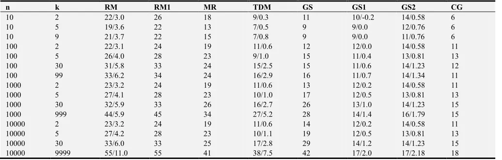
Table 2 provides a comparison of the methods that were mentioned earlier:
a)RM – the Richardson method with optimal %, (% is calculated in the numerical experiment),
b)RM1 – the Richardson method with % = 0.5 (K K=+
p),
c)MR – the minimum residual method % =,,-./,
--.,-,
d)TDM – the tri-diagonal method with optimal %, e)GS – the Gauss-Seidel method (% = 0), f) GS1 – the Gauss-Seidel method with optimal %,
g)GS2 – the Gauss-Seidel method with
% = 0.5 (•pK K=− p), (% is an approximation of
%ijk for the Gauss-Seidel method – see Remark 5).
Because XX= 2, for R = 1,2, … , , this algorithm is equivalent to the new variant of the Gauss-Seidel method (Remark 8),
h)CG – the conjugate gradient method.
Table 2. Comparison of the number of iterations for different values n and k. The notation NI/q denotes: NI – number of iterations, q – the value of % used in the given iterative process.
n k RM RM1 MR TDM GS GS1 GS2 CG
10 2 22/3.0 26 18 9/0.3 11 10/-0.2 14/0.58 6
10 5 19/3.6 22 13 7/0.5 9 9/0.0 12/0.76 6
10 9 21/3.7 22 15 7/0.8 9 9/0.0 11/0.76 6
100 2 22/3.1 24 19 11/0.6 12 12/0.0 14/0.58 11
100 5 26/4.0 28 23 9/1.0 15 11/0.4 13/0.81 13
100 30 31/5.8 33 24 15/2.5 15 11/0.6 14/1.23 12
100 99 33/6.2 34 24 16/2.9 16 11/0.7 14/1.34 11
1000 2 23/3.2 24 19 11/0.6 13 12/0.2 14/0.58 11
1000 5 27/4.1 28 23 10/1.0 17 12/0.5 13/0.81 13
1000 30 32/5.9 33 26 16/2.7 26 13/1.0 14/1.23 15
1000 999 44/5.9 45 34 27/5.2 28 14/1.4 16/1.79 15
10000 2 23/3.2 24 19 11/0.6 14 12/0.2 14/0.58 11
10000 5 27/4.2 28 23 10/1.1 19 12/0.5 13/0.81 13
10000 30 33/6.0 33 25 17/2.8 29 14/1.2 14/1.23 15
6. Conclusions
A new approach to the simple iterative methods is done. Owing to introducing a new parameter q the Jacobi, Richardson, Gauss-Seidel methods are convergent for every linear system with a positive definite matrix. The optimality criterion for the parameter q is given. Thus, interesting results for the Jacobi, Richardson and Gauss-Seidel method are obtained. The Gauss-Seidel method with the parameter %, in a sense, is equivalent to the SOR method. From the formula for the optimal value of % results the formula for optimal value of . Up to present, this formula was known only in special cases. Practical useful approximate formula for optimal value is also given. Numerical experiments confirm: for very large scale systems the speed of convergence of the SOR method with optimal or approximate parameter is near the same as the speed of convergence of conjugate gradients method.
References
[1] I. Koutis, G. L. Miller, R. Peng, A fast solver for a class of linear systems, Communications of the ACM 55 (10) (2010) 99-107.
[2] E. G. Boman, B. Hendrickson, S. Vavasis, Solving elliptic finite element systems in near-linear time with support preconditioners, SIAM J. Numer. Anal. 46 (6) (2008) 3264-3284.
[3] J. D. Hogg, J. A. Scott, A fast and robust mixed-precision solver for the solution of sparse symmetric linear systems, ACM Trans. on Math. Soft. 37 (2) (2010).
[4] J. Stoer, R. Bulirsch, Introduction to Numerical Analysis, Third Ed., Springer Verlag, 2002.
[5] Y. Saad, Iterative Methods for Sparse Linear Systems, Second Ed., SIAM Press, 2016.
[6] D. S. Watkins, Fundamentals of Matrix Computations, Second Ed., Wiley, 2002.
[7] D. M. Young, Iterative Solutions of Large Linear Systems, Academic Press, New York, 1971, reprinted by Dover 2003. [8] C. G. Broyden, On the convergence criteria for the method of
successive over-relaxation, Mathematics of Computation 18 (85) (1964) 136-141.
[9] S. Yang, M. K. Gobbert, The optimal relaxation parameter for the SOR method applied to the Poisson equation in any space dimensions, Appl. Math. Letters, 22 (2009) 325-331.
[10] J. W. Demmel, Applied Numerical Linear Algebra, SIAM Press, 1997.
[11] I. K. Youssef, S. M. Ali, M. Y. Hamada, On the Line Successive Overrelaxation Method, Applied and Computational Mathematics, 5, 3 (2016) 103-106.
[12] Cheng-yi Zhang, Zichen Xue, A convergence analysis of SOR iterative methods for linear systems with week H-matrices, Open Mathematics, 2016.
[13] S. Karunanithi, N. Gajalakshmi, M. Malarvishi, M. Saileshwari, A Study on comparison of Jacobi, Gauss-Seidel and SOR methods for the solution in system of linear equations, Int. J. of Math. Trends and Technology, (IJMTT), 56, 4, 2018.
[14] O. Nevanlinna, How fast can iterative methods be? In “Recent Advances in Iterative Methods”, ed. by G. Golub, A. Greenbaum, M. Luskin, Math. and its Appl., 60 (2012) 135-148.