Errors of Misclassification Associated with Edgeworth Series Distribution (ESD)

http://www.sciencepublishinggroup.com/j/ajtas doi: 10.11648/j.ajtas.20190806.12

ISSN: 2326-8999 (Print); ISSN: 2326-9006 (Online)

Errors of Misclassification Associated with Edgeworth

Series Distribution (ESD)

Awogbemi Clement Adeyeye

*

, Onyeagu Sidney Iheanyi

Statistics Department, Nnamdi Azikiwe University, Awka, Nigeria

Email address:

*

Corresponding author

To cite this article:

Awogbemi Clement Adeyeye, Onyeagu Sidney Iheanyi. Errors of Misclassifications Associated with Edgeworth Series Distribution (ESD). American Journal of Theoretical and Applied Statistics. Vol. 8, No. 6, 2019, pp. 203-213. doi: 10.11648/j.ajtas.20190806.12

Received: March 2, 2019; Accepted: March 30, 2019; Published: November 8, 2019

Abstract:

This study investigates the errors of misclassification associated with Edgeworth Series Distribution (ESD) with a view to assessing the effects of sampling from non-normality. The effects of applying a normal classificatory rule when it is actually a persistent non-normal distribution were examined. These were achieved by comparing the errors of misclassification for ESD with ND using small sample sizes at every level of skewness factor. The simulation procedure for the experiment of the study was implemented using numerical inverse interpolation method in R program to generate a uniformly distributed random variable N. A configuration size of 1000 was obtained for the two training samples drawn at every level of skewness factor (λ3), in the range (0.00625, 0.4). This was repeated for different small sample sizes by comparing errors of

misclassification of ESD with ND. The simulation results showed that the optimum probabilities of misclassification by ESD: (E12E) decreases and (E12E) increases, as the skewness factor (λ3) increases. The optimum total probability of misclassification

is stable as λ₃ also increases. The probability of misclassification E12E ≥ E12N and E21E ≥ E21N at every level of λ3. Thus, the

total probabilities of misclassification are not greatly affected by the skewness factor. This asserts that the normal classification procedure is robust against departure from normality.

Keywords:

Errors of Misclassification, Edgeworth Series Distribution, Skewness Factor, Classificatory Rule, Optimum Probability of Misclassification

1. Introduction

1.1. Background to the Study

The study of discrimination and classification problems with a view to assessing the effects of departure from the usual assumptions of normality cannot be overemphasized. In discrimination, we are concerned with the existence of two or more groups and a sample of observations from each of the groups. We are therefore required to design a rule based on measurements from these observations to the correct population when we do not know from which of the two populations it emanates [1, 22].

Classification is concerned with prediction or allocation of observations into groups in which a sample of observations is also given. The problem is to classify the observations into groups which are as distinct as possible [16].

Classification problem occurs when a researcher makes a

number of measurements on observations and wishes to classify the observations into one of several groups on the basis of the measurements. The observations cannot be identified with a group directly without recourse to the measurements. Fisher [8], illustrating this concept, classified iris flower from unknown group (specie) to any of the three known species (Iris Setosa red, Iris Versicolour green, and Iris Virginica black) on the basis of their attributes (Sepal length in cm, Sepal width in cm, Petal length in cm and Petal width in cm).

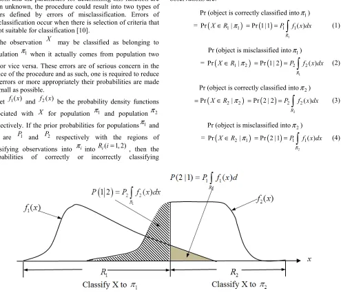
random and the parameters for determining this function are often unknown, the procedure could result into two types of errors defined by errors of misclassification. Errors of misclassification occur when there is selection of criteria that is not suitable for classification [10].

The observation X may be classified as belonging to population π1 _{when it actually comes from population two}

2

π _{or vice versa. These errors are of serious concern in the} choice of the procedure and as such, one is required to reduce the errors or more appropriately their probabilities are made as small as possible.

Let f x1( ) _and f2( )x _{be the probability density functions} associated with X for population π1 _{and population}π2 respectively. If the prior probabilities for populationsπ1 _and

2

π _are P1 _and P2 _{respectively with the regions of}

classifying observations into πi _into R ii( =1, 2) _{, then the}

probabilities of correctly or incorrectly classifying

observations are:

Pr (object is correctly classified intoπ₁)

=

(

)

( )

1

1 1 1 1

Pr | Pr 1 | 1 ( )

R

X∈R π = =P

∫

f x dx (1)

Pr (object is misclassified intoπ₁)

=

(

)

( )

1

1 2 2 2

Pr | Pr 1 | 2 ( )

R

X∈R π = =P

∫

f x dx (2)

Pr (object is correctly classified intoπ₂)

(

)

( )

2

2 2 2 2

Pr | Pr 2 | 2 ( )

R

X R π P f x dx

= ∈ = =

∫

(3)

Pr (object is misclassified intoπ₂)

=

(

)

( )

2

2 1 1 1

Pr | Pr 2 | 1 ( )

R

X∈R π = =P

∫

f x dx (4)

Figure 1. Probabilities of Misclassification.

In constructing a classification procedure, it is needful to minimize on the average, the bad effects of misclassification since a good classification procedure results to few misclassifications [18].

The Linear Discriminant Function (LDF) is a statistical procedure constructed as

(

1 2

)

1 1

(

1 2

)

1

. 2

X

µ µ

_{− Σ}−  ₋

µ µ

₋ 

 

  It

assigns p dimensional observation vector X into one of the two populations π_i (i = 1, 2) and it is employed as an assignment rule when:

(a)The density functions of observations from populations 1

π and π₂ are multivariate normal:

( , ),

1,2

N

p

i

i

i

π

µ

Σ =

(b)The variance-covariance matrix (Σ1) in population π1 is the same as Σ₂in population

π

₂;

(c)The prior probabilities of observations coming from

populations π₁andπ₂ are known;

(d)The parameters of the density functions in (a) are known.

Suppose the assumptions specified above are satisfied, then the Linear Discriminant Functions (LDF) provides optimal assignment rule in that it cannot be improved upon and the errors of misclassification are minimized. However, when some or all the assumptions are violated, it would be of interest to researchers to determine the effects of the violation on the procedures using LDF. If the parameters in (a) above are estimated from the samples, two problems may arise from the estimation stage. We may have missing values in the data and the initial sample may not be properly assigned due to inaccuracy in the initial assignment.

1.2. Statement of the Problem

regions for classification. The question that emanates is: “how does this failure to transform to normality, prior to classification, affect the probability of misclassification”? This problem was investigated by comparing the errors of misclassification associated with Johnson’s system distributions in the appropriate transformable non-normal case with that of normal distribution [6]. Errors of misclassification associated with Gamma were also examined by [15]. Considerable work has been done by researchers in connection with errors of misclassification when the underlying distribution is transformable non-normal distribution, but the errors of misclassification associated with persistent non-normal distribution remain unresolved [12].

For any classification rule, the associated error rates are often used as criteria for evaluation of classification performance. These error rates are easily calculated when population parameters are known. However, when these parameters are unknown and must be estimated from the samples, the exact overall expected rate for the Fisher’s Linear Discriminant Function becomes virtually intractable. There is also a loss of information which affects the estimation of the probabilities of misclassification, in that it may be underestimated or overestimated. In order to rectify this problem, we derive the asymptotic distribution for the expected probability of misclassification of the distribution under consideration [17].

The aim of this study is to investigate errors of misclassification associated with Edgeworth Series Distribution (ESD). The research work seeks to achieve the following objectives:

i. To examine the effect of applying the normal classificatory rule when the distribution is ESD by comparing the errors of misclassification using the Normal Distribution (ND) and ESD classification rules. ii.To use simulated data to validate the established results

of the study.

2. Literature Review

The problem of estimating probabilities of misclassification has received remarkable attention in the literature ever since [8] introduced the Linear Discriminant Function. An extensive bibliography on this subject has been published by [21] since the probabilities of misclassification provide a way of evaluating the performance of the classification procedure.

Several investigations have also been conducted on the effects of non-normality on classification rules:

The robustness of the LDF and QDF with respect to certain types of non-normality was studied by [4], considering Johnson’s system of distributions which are transformable to normality. They considered three members of the family: log normal transformation

log( ), 0

Y

i

=

x

i

< < ∞

x

i

, Logit normal transformation

1

log i ,0 1

i

x x

Y_i   x_i

−

 

= < < and Inverse hyperbolic sine normal

transformation

Y

sin ( ),

1

x

x

i

=

−

i

−∞ < < ∞

i

. Sampling studies

were conducted in order to examine the behavior of the errors of misclassification, and they found out that the total error of misclassification is greatly increased as individual errors are distorted for all transformations in the case of the LDF. Approximate minimax rules were investigated because of the distortion in the errors and are found to reduce the errors of misclassification greatly.

The effect of non-normality on the QDF was investigated by [13]. They assumed that the data were transformable to normality. They derived random samples from non-normal distributions in order to study the effect of non-normality on QDF. Their results indicated that the actual error rates were considerably larger than the optimal rates in the case of zero mean difference.

The robustness of the Linear Discriminant Function (LDF) to non-normality using three Johnson system’s of distributions was examined by [6]. Though their work was restricted to transformable normality only, they opined that further work be carried out on a distribution that is non-normal with robustness on small sample sizes.

The effect of applying normal classificatory rule with focus on non-normality was also examined by [12]. He also obtained the asymptotic distribution of errors of misclassification in the non -normal case using Johnson’s system of distribution. The distribution function G z₁( ) and the expected value of the conditional distribution E e

( )

₁₂

were evaluated for various values of given parameters theoretically using Johnson system of distributions. It was observed that the presence of outliers in one sample does not affect the behavior of the error rates in general.

Errors of misclassification for classification problems with two classes of univariate-gamma distribution were studied by [15]. The gamma density functions given as

( )

( )

i 1_exp

(

)

_{, 1, 2}

i i

f x x x i

θ θ

λ _λ

θ −

= − =

Γ (5)

were reparameterized to the form

(

)

( )

1

, , exp , , 0,

i i i

i

x

f x x

θ

θ

θ

µ θ

θ µ µ θ

θ − µ

 

  _{ }

 

= −  >

Γ  

(6)

The effects of applying the normal classificatory rule to non-normal transformable gamma distribution were studied and assessed by comparing probabilities of misclassification (optimum and conditional). This was based on the Linear Discriminant Function (LDF) for normality and the likelihood ratio rule (LR) for gamma populations for various combination of λ λ₁, ₂ and θ. They concluded that for small values of θ, n1 and n2, the distribution functions do not

In this study, we examine the persistent non-transformable, non-normal distribution by investigating the effects of applying the normal classificatory rule when the distribution is ESD using empirical approach. We also develop expected probability of misclassification for ESD and its asymptotic distribution.

3. Method

The effects of non-normality in a two population discriminatory problem on the errors of misclassification are examined when the Anderson’s statistic (W) defined by means of Edgeworth Series Distribution (ESD) is used for classifying an observation as emanating from population π₁ or π₂.The effects would be studied for varying values of skewness factor based on the boundary of unimodal region for Edgeworth Series Distribution.

Optimum probabilities of misclassification for ESD are computed from known parameters and subsequently, the apparent probabilities of misclassification in respect of ESD for known and estimated parameters are generated.

3.1. Edgeworth Series Distribution (ESD)

Edgeworth Series Distribution (ESD) constitutes an expansion which is a series that approximates a probability distribution in terms of its cumulants and the Hermite polynomials. It relates the probability density function to that of a standard normal distribution [19].

The use of ESD is expedient because approximations to distribution of sample statistics of higher order than

1 2

n− is of concern interest in asymptotic theory of statistics. An important tool that evaluates the refinements is provided for by ESD. Its expansions take cognizance of a method of using information about a higher order moment to increase approximations accuracy [17].

Let F(x) be the distribution to be approximated,

{ }

k_n its cumulants, γ_k the cumulants of a standard normal distribution function and D the differential operator with respect to x. Also, let Φ and φ be the standard normal distribution and standard normal density function respectively. Then

F(x) = exp

(

) ( )

_{( )}

1 n!

n

n n x

n

D k γ

∞

=

−

− Φ

∑

(7)

This is identical with the expansions in Hermite orthogonal function for a probability density function

( )

( )

0

(x)

k n n

P x c H φ x

∞

=

=

∑

(8)

whereH_{( )n} are Hermite polynomials and

( )

( )

( )

1 !

k n

C P x H x dx k

∞ −∞

=

∫

(9)

By considering the standardized sum of n independent and identically distributed random variables, Edgeworth Series is obtained by collecting terms in equation (10) according to the power of n [11].

Let X X_{1, 2,}...X_n be independent and identically distributed random variables with mean θ₀ =µ and finite variance σ2. If

θ

$n is constructed from a sample of size n and

$

1 2

0

( n )

n− θ −θ is asymptotically and normally distributed, then Edgeworth Series expansions are developed as approximations to distribution of estimates θ_n of unknown quantities θ₀. Thus the distribution functions of

$

1 2

0

( n )

n− θ −θ is expanded as a power series in 1 2

n− _{so that}

$

(

)

1

2 1

2 0

2

1 2

( ) ( ) ( ) ... n ( ) ( ) ...

j n

n

P θ θ x x

n P

xφ x P xφ x

σ

− −

+

 

 ₋ 

 _≤ _{= Φ + + +}

 

 

 

(10)

where φ( )x =

( )

2

2

1

1 ₂

2 2

x

e σ

σ− π − − _{is the standard normal} density function

and ( )x

Φ = ( )

x

x du φ

−∞

∫

is the standard normal distribution

function

Equation (10) is the Edgeworth Series expansion. The functions Pj are polynomials with coefficients depending on

cumulants of θ$n−θ₀. In particular, Pj is a polynomial of

degree at 3j -1.

Suppose X_ij,i=1, 2, j=1, 2,K,n_{i denote two}

independent random samples from populations π_i,i=1, 2 respectively. The observations Xij emanate from the

common distribution defined by the density function

3 3

( ) 1 , 1, 2

6

i i

x

f x λ D φ µ x i

σ

  _{ − }

= −_ _{  } − ∞ < < ∞ =

 

  (11)

The parameter λ µ =₃, _i(i 1, 2) satisfies the conditions:

3 , i

λ µ

−∞ < < ∞ − ∞ < < ∞ and, where D denotes the

differential operator d

dx,

( )

1

(

)

2 2

2 2

exp 2

i

x

x

i

π µ

σ σ

µ

φ σ

_ _= − − − 

 

  _{ }

−

and

λ

3 is the skewness factor [4].

3.2. Proposed Method of Estimating Probabilities of Misclassification

Let X_ij,i=1, 2;j=1, 2...n_i be independent samples of sizes n n₁, ₂ from populations π1, π2. To estimate the apparent

probabilities of misclassification, we define

1

12

1 1

n j E

j

E

n

γ

=

=

∑

(13)

where

γ

_j=1ifX1j is classified as belonging to π2 and γi =0

if X1j is classified as belonging to π1,j=1, 2,...n1.

The sample X₁₁,...X_1n is taken from π₁ and each observation is classified in accordance with the rules in equations (35) and (36).

Similarly,

2

21

2 1

n j E

j

E

n

δ

=

=

∑

(14)

where

δ

_j=1if X2j is classified as belonging to π1 and

0

j

δ

= if X2j is classified as belonging to π2, j=1, 2,...n2 The sample X₂₁,...X_2n is taken from π₂ and each observation is classified in accordance with the rules in equations (35) and (36).

The notation E12E and E21E represent the apparent

probabilities of misclassification when observations from populationsπ₁andπ₂ are misclassified respectively by ESD rule.

For the purpose of comparison, the classification rule in equation (37) is successively applied to X1j,X2j. The

proportion misclassified is estimated by the same procedure. Thus,

1

12

1 1

n j N

j

E

n

γ

=

=

∑

(15)

And

2

21

2 1

n j N

j

E

n

σ

=

=

∑

(16)

represent the two errors of misclassification. 3.3. Classification Rules for Normal Distribution

Let the probability density function of X inπ_i(i=1, 2) be

1 1

( ) exp[ ], , 1, 2

2 2

i i

x

f x

µ

x i

σ

σ π

−

 

= −   −∞ < < ∞ =

  (17)

If

θ

is the mean of the observation X and

1 2

:

:

0

H

θ µ

=

vs Ha

θ µ

=

, then the likelihood when

1 2

µ µ

<

2 2

1 1 2

2

2 2

1 1 2

( ) 1 1

exp

( ) 2 2

1 1

2 2

f x x x

L f x

x x

L

µ

µ

σ

σ

µ

µ

σ

σ

 _{ −   − } 

 

= = −   +  

     

 

− −

   

= −   +  

    (18)

(

) (

)

(

)

1 2 2 1

2

1 2

1 2

1 2 2

1 2

x

x

µ µ

µ

µ

σ

µ µ

µ µ

σ

 

= − _ − + _ −

−

 

 

=_ − + _{ }  

(19)

Equation (19) is the Anderson’s discriminant function (W) when the distributions in the two populations are univariate normal with the same variance but different means [20]. We reject H0 if L< K, where K is a constant.

From Equation (19) and the decision rule made, the classification rule specifies as follows:

1 2

0

0

Classify X

if W

Classify X

if W

π

π

∈

>

∈

≤

(20)

Equation (20) reduces to

(

)

(

)

1 1 2

2 1 2

1 2 1 2

Classify X if X

Classify X if X

π µ µ

π µ µ

∈ < +

∈ ≥ +

(21)

Similarly, when µ₁>µ₂ the classification rule becomes

(

)

(

)

2 1 2

1 1 2

1 2 1 2

Classify X if X

Classify X if X

π µ µ

π µ µ

∈ < +

∈ ≥ +

(22)

When the parameters

µ µ

_{1, 2} are unknown, and estimated by X X₁, ₂ from the sample sizes ofn and n_{1 2} respectively, the classification rule becomes:

1 2

1 1 2

1 2

1 1 2

, 2

, 2

X X

Classify X if X X X

and

X X

Classify X if X X X

π

π

+

∈ < <

+

∈ > ≥

(

1 2

)

2 1 2

1 2

2 1 2

, ,

2

, 2

X X

Similarly X if X X X

X X

and classify X if X X X

π

π

+

∈ ≥ <

+

∈ ≤ ≥

(24)

3.4. Classification Rule for Edgeworth Series Distribution (ESD)

Let the pdf of X in

π

i

be

3 3

( ) 1 , , 1, 2

6

i i

x

f x λ D φ µ x i

σ −

   

= −    −∞ < < ∞ =

   

(25)

When µ₁<µ₂, the likelihood ratio becomes

3

3 1 3 1 1

3 3

1

3

2 _{3 2 3 2 2}

3 3 1 2 6 ( ) ( ) 1 2 6

x x x

f x L

f x _{x x x}

λ µ λ µ _φ µ σ σ σ σ σ λ µ λ µ _φ µ σ σ σ σ σ  _{  −    − }  _{ − } − +                         = =  _{  −    − }  _{ − } − +  _ _ _ _{ }_ _  _{ }     (26)

Equation (26) becomes

2 1 2 2 1 exp 2 1 exp 2 x P L x Q µ σ µ σ  _{ − }  −  _{ }        =  _{ − }  −  _{ }        (27) 3

3 1 3 1

3 3

1

2 6

x x

where P λ µ λ µ

σ σ σ σ  _{ −   − }    = −  +           (28) and 3

3 2 3 2

3 3

1

2 6

x x

Q λ µ λ µ

σ σ σ σ  _{ −   − }    = −  +           (29)

We reject H0 by if

ln L < K (30) Taking K =1 reduces equation (30) to ln L< 0

Thus, we reject X∈π₁if

2 2

1 2

1 2 1 2

2

1 1

ln ln 0

2 2

ln 0

2

x x

P Q

This reduces to P x Q µ µ σ σ µ µ µ µ σ − −    

−   − +   <

   

 

   ₊   ₋ 

+ − <

      

   

   

(31)

From equation (30), the classification rule takes the form:

1 2 1 , ln 0 For P

classify X if W

Q

µ µ

π <

 

∈  + >

  (32) and 2 1 2 1 ln 0 , ln 0 P

classify X if W

Q

For

P

classify X if W

Q π µ µ π   ∈  + ≤   >  

∈  − >

 

(33)

and

2 ln 0

P classify X if W

Q

π  

∈  − ≤

  (34)

When the parameters µ µ₁, ₂ are unknown, they are estimated by X1,X2 respectively and plugged in equation

(34) before classification begins.

In the process of comparing errors of misclassification using ESD and ND classification rules, and data generated from the ESD, the effect of applying normal classification rule(likelihood ratio) when the distribution is ESD would be investigated by empirical method. Thus, the classification rule for ESD is given in the form:

1 2 2 1 1 ₂ 2 , 1 exp 2 1 1 exp 2 For x P

classify X if

x Q µ µ µ σ π µ σ <  _{ − }  −  _{ }        ∈ <  _{ − }  −  _{ }        (35) and 2 1 2 ₂ 2 1 exp 2 1 1 exp 2 x P

classify X if

x Q

µ

σ

π

µ

σ

 _{ − }  −  _{ }        ∈ ≥  _{ − }  −  _{ }        (36)

where P and Q remain as earlier defined in equations (35) and (36)

The normal classificatory rule for µ₁<µ₂ is

1 2

1

2

2 classify X if X

and

classify X if otherwise µ µ π

π

+

 

∈ < 

 

∈

3.5. Comparison of Errors of Misclassification

We estimate the errors of misclassification with focus on the small sample sizes. This is based on the fact that the asymptotic expansion of the errors does not indicate the behaviour of the error for small sample sizes [5, 9].

Estimation of the optimum probability of misclassification in the ESD when the skewness factor is in the range (0.00625, 0.4) is considered.

The apparent error rate for the Normal Distribution and ESD classification rules are examined using simulated data from ESD. The classification rules for the two distributions are also derived using likelihood criterion. The form of the estimators and the choice of values for skewness factor are also presented. The errors of misclassification are subsequently compared using the likelihood ratio rules for the Normal Distribution and ESD.

3.6. Choice of Skewness Factor Values

The choice of the values for skewness factor (λ₃) is anchored on the boundary of the positive unimodal regions for ESD where its probability density function is only valid. Thus, the skewness factor is chosen to lie within the range

(

0.00625, 0.4

)

as suggested by [3, 7].

3.7. Optimum Probability of Misclassification of ESD

When all the parameters of the distributions in the populations are known, the probability of misclassification is optimal in the sense that we cannot improve upon it. When an observation from π₁ is misclassified, the optimum probability of misclassification is given by

[ ]

(

1 2

)

1

3

3 1

3 1 1

3 3

3

1 1 1

3 3 , Pr 2 1 6 1 6 6

R f X

x

D dx

x x

H dx

x x x

dx H dx

δ δ δ δ µ µ α λ _φ µ σ λ µ _φ µ σ σ σ λ µ µ µ φ φ σ σ σ σ ∞ ∞ ∞ ∞  ₊  =  ≥      −     =  −          −   −  =  +           − − −       =   +          

∫

∫

∫

∫

(38)

where 1 2

2

µ µ

δ

= + 

  and Hn( )x is Chebyshev’s-Hermite

polynomial of degree r and defined by the identity: ( ) ( ) ( )n ( )

n

H x

φ

x = −D

φ

x (39) See [11].

If φ( )x denotes the standard normal density function, then we define the Hermite polynomial H_n( )x for any integer n by

( )

2

2 ( 1)

1 ( ) ( ) ( )

2

t

n n n

n itx

n

n n

d d

e e dt x H x x

dx dx φ φ

π

∞ −

−∞

− _{= − =}

∫

(40)

and setting z x

µ

1

σ

−

= as in equation (38), we have

[ ]

1 1

3

1 2 3

3

1 1 1

2 2

3

2 1 2 1 2 1

2 , ( ) ( ) ( ) 6 1 6 1 1

2 6 2 2

R f z dz H z z dz

H δ µ δ µ σ σ λ α φ φ σ λ δ µ δ µ δ µ φ φ σ σ σ σ λ µ µ µ µ µ µ φ φ σ σ σ σ ∞ ∞ − − = + − − −       = −  +             − − −       = −  +  −          

∫

∫

(41)

If an observation from π2is misclassified, the optimum probability of misclassification is given by

[ ]

(

1 2

)

2

3

3 2

3

2 2 2

3 3 , Pr 2 1 6 6

R f X

x

D dx

x x x

H dx δ δ δ µ µ α λ _φ µ σ λ µ µ µ φ _{σ σ} φ _σ σ −∞ −∞ −∞  ₊ 

=  < 

    −     =  −        − − −       =  +          

∫

∫

∫

(42)

where

(

1 2

)

2 µ µ δ = + .

Using the result in equation (38) and setting z x

µ

2

σ

−

= ,

we have

[ ]

( 2) 3 ( 2)

2 2 3

3

2 2 2

2 2

2 3

1 2 1 2 1 2

2

, Pr ( ) ( ) ( )

6

6

1

2 6 2 2

R f z dz H z z dz

H δ µ δ µ σ λ σ α φ φ σ λ δ µ δ µ δ µ φ _{σ σ} φ _σ σ λ µ µ µ µ µ µ φ φ σ σ σ σ − − −∞ −∞ = + − − −       = _{ }− _{   }         − − −   _  _   = _{ }− __ _ − _ _ _  

∫

∫

(43)

4. Results

The optimum probabilities of misclassification are generated from equations (41) and (42). We assume that the known parameters: µ1=0,µ2=1and

2 1

σ = . This implies that equations (41) and (42) are now functions of the skewness factor

( )

λ

₃ in the range

(

0.00625, 0.4 .

)

The probabilities of misclassification

(

E_12E andE_21E

)

are also computed and the results displayed in Table 1.

The apparent probabilities of misclassification are also examined when µ1andµ2 are known and when the parameters are estimated from the samples.

Two independent samples of configuration size of 1000 each are at each value of the skewness factor

( )

λ

₃ from populations π1 and π2. Their distributions are of ESD with

respective parameters

µ

₁=0,

σ

2=1,

µ

₂=1and.

misclassification obtained from the samples are averaged and the results displayed in Tables 2-6.

The notation E_12E is the apparent probability of misclassification when an observation from π₁ is misclassified by ESD and E_21E is the apparent probability of misclassification when an observation from π₂ is misclassified by ESD. Similarly, E_12N and E_21N are apparent probabilities of

misclassification when observation from populations π₁ and 2

π are misclassified respectively by ND classification rule. The simulation experiments have been implemented using R programs and all the simulation results are obtained and displayed along with the total probabilities of misclassification in Tables 1-6.

Table 1. Optimum Probabilities of Misclassification at Different Values of Skewness for ESD.

Skewness Factor (λ3)

Optimum Probability of Misclassification

E12E E21E Total

0.00625 0.3082 0.3088 0.6170

0.0125 0.3079 0.3091 0.6170

0.025 0.3074 0.3096 0.6170

0.05 0.3063 0.3107 0.6170

0.10 0.3041 0.3129 0.6170

0.15 0.3019 0.3151 0.6170

0.20 0.2997 0.3173 0.6170

0.25 0.2975 0.3195 0.6170

0.30 0.2953 0.3217 0.6170

0.35 0.2931 0.3239 0.6170

0.40 0.2909 0.3261 0.6170

The results in Table 1. show that E_12Edecreases as the skewness factor λ₃ increases and E_21E increases as λ₃ increases. The total probability of misclassification is also stable (constant) as

λ

3 increases.

Table 2. Comparison of Errors of Misclassification for Means unknown and Estimated by Average Values over 5 Samples.

Skewness Factor (λ3)

ESD ND

E12E E21E Total E12N E21N Total

0.00625 0.140 0.400 0.540 0.140 0.400 0.540

0.0125 0.220 0.410 0.630 0.220 0.410 0.630

0.025 0.225 0.465 0.690 0.220 0.475 0.695

0.05 0.210 0.395 0.605 0.205 0.400 0.605

0.10 0.205 0.475 0.680 0.175 0.495 0.670

0.15 0.260 0.285 0.545 0.230 0.320 0.550

0.20 0.305 0.365 0.670 0.295 0.395 0.690

0.25 0.455 0.185 0.640 0.420 0.230 0.650

0.30 0.195 0.465 0.660 0.115 0.545 0.660

0.35 0.225 0.465 0.660 0.125 0.520 0.645

0.40 0.440 0.180 0.610 0.360 0.250 0.610

From Table 3, E12E is either equal to or greater than E12N and E21E is either equal to or less than or greater than E21N at every

level of skewness factor. The equality of the probability also occurs when the skewness factor λ3 is very small.

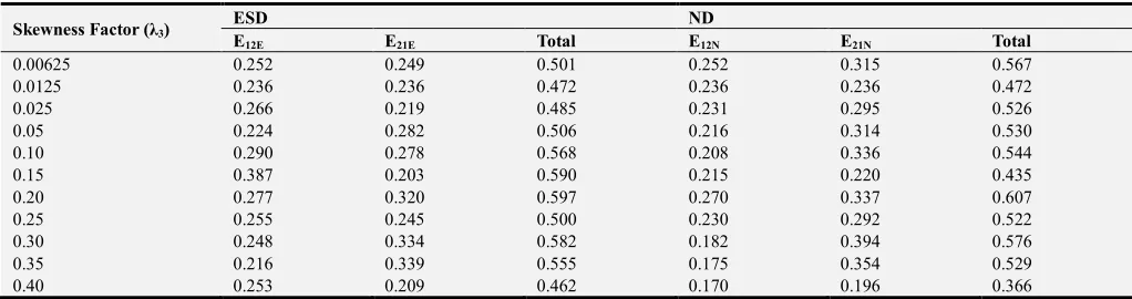
Table 3. Comparison of Errors of Misclassification for Means unknown and Estimated by Average Values over 10 Samples.

Skewness Factor (λ3)

ESD ND

E12E E21E Total E12N E21N Total

0.00625 0.252 0.249 0.501 0.252 0.315 0.567

0.0125 0.236 0.236 0.472 0.236 0.236 0.472

0.025 0.266 0.219 0.485 0.231 0.295 0.526

0.05 0.224 0.282 0.506 0.216 0.314 0.530

0.10 0.290 0.278 0.568 0.208 0.336 0.544

0.15 0.387 0.203 0.590 0.215 0.220 0.435

0.20 0.277 0.320 0.597 0.270 0.337 0.607

0.25 0.255 0.245 0.500 0.230 0.292 0.522

0.30 0.248 0.334 0.582 0.182 0.394 0.576

0.35 0.216 0.339 0.555 0.175 0.354 0.529

From Table 3, E12E is either equal to or greater than E21Nand E21E is also equal to or less than E21N at every level of skewness λ3. Table 4. Comparison of Errors of Misclassification for Means unknown and Estimated by Average Values over 15 Samples.

Skewness Factor (λ3) E12E E21E Total E12N E21N Total

0.00625 0.345 0.145 0.490 0.345 0.150 0.495

0.0125 0.310 0.310 0.620 0.310 0.310 0.620

0.025 0.405 0.280 0.685 0.400 0.285 0.685

0.05 0.230 0.390 0.620 0.225 0.395 0.620

0.10 0.375 0.305 0.680 0.350 0.315 0.665

0.15 0.405 0.180 0.585 0.360 0.225 0.585

0.20 0.355 0.325 0.680 0.320 0.355 0.675

0.25 0.295 0.340 0.635 0.235 0.395 0.630

0.30 0.320 0.350 0.670 0.230 0.385 0.615

0.35 0.260 0.345 0.605 0.200 0.430 0.630

0.40 0.315 0.375 0.690 0.145 0.415 0.560

From Table 4, E12E is equal to or greater than E21N and E21E is either less or greater than or equal to E21N at every level of

skewness factor λ3.

Table 5. Comparison of Errors of Misclassification for Means unknown and Estimated by Average Values over 20 Samples. Skewness Factor (λ3) E12E E21E Total E12N E21N Total

0.00625 0.220 0.206 0.426 0.220 0.206 0.426

0.0125 0.280 0.280 0.560 0.192 0.295 0.487

0.025 0.330 0.210 0.540 0.290 0.230 0.520

0.05 0.345 0.205 0.550 0.295 0.250 0.545

0.10 0.265 0.300 0.565 0.230 0.390 0.620

0.15 0.340 0.350 0.690 0.330 0.375 0.705

0.20 0.350 0.240 0.590 0.320 0.255 0.575

0.25 0.295 0.270 0.565 0.270 0.295 0.565

0.30 0.300 0.195 0.495 0.265 0.200 0.465

0.35 0.310 0.350 0.660 0.270 0.360 0.630

0.40 0.405 0.285 0.690 0.380 0.400 0.780

From Table 5, E12E is either equal to or greater than E12N and E21E is either equal to or less than E21Nat every level of

skewness λ3.

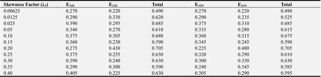
Table 6. Comparison of Errors of Misclassification for Means unknown and Estimated by Average Values over 25 Samples. Skewness Factor (λ3) E12E E21E Total E12N E21N Total

0.00625 0.270 0.220 0.490 0.270 0.220 0.490

0.0125 0.290 0.330 0.620 0.290 0.235 0.525

0.025 0.390 0.295 0.685 0.375 0.310 0.685

0.05 0.340 0.270 0.610 0.335 0.280 0.615

0.10 0.375 0.305 0.680 0.360 0.315 0.675

0.15 0.360 0.230 0.590 0.345 0.245 0.590

0.20 0.275 0.430 0.705 0.225 0.480 0.705

0.25 0.375 0.255 0.630 0.320 0.290 0.610

0.30 0.390 0.240 0.630 0.300 0.330 0.630

0.35 0.290 0.300 0.590 0.240 0.345 0.585

0.40 0.405 0.225 0.630 0.305 0.290 0.595

From Table 6, E12E is equal to or greater than E12N and E21E

is either equal to or greater than E21N at every level of

skewness λ3.

5. Discussion

From the simulation results, It is evident that the total probability of misclassification at every value of

λ

₃is either under or overestimated when small samples are employed to estimateµ₁ andµ₂. The differences between taking small sample sizes are also not apparent.

The fact that E_12E ≥E_12Nand E_21E ≤E_21Nat every level

of skewness factor needed some algebraic justification and that has been established in this study. The actual probabilities of misclassification E12E and E21E as well as

their sum remain close to the corresponding errors induced by the normal rule when

λ

3is small. As

λ

3 increases, E12E

tends to be larger than E12N and E21E is smaller than E21N.

Also, from Tables 4-6, the total probabilities of misclassification for the ESD and ND classification rules indicate no major difference between them at each value of

3

that for small sample sizes, E_12E ≥E_12Nand E_21E ≤E_21N . The observed equality occurs when

λ

₃ is very small with an increasing parity as λ₃ increases. The observed equality of probabilities requires some algebraic justification.

From Normal Distribution (ND) classification rule and ESD classification rule, we earlier specified that

3

3 3

3 3

1

2 6

X X

P λ µ λ µ

σ σ

σ σ

 _{  −    − } 

= − _{  }+_{  } 

   

   

 

 

(44)

3

3 2 3 2

3 3

1

2 6

X X

Q λ µ λ µ

σ σ

σ σ

 _{  −    − } 

 

= −  +  

       

 

(45)

When µ₁=0,µ₂ =1and σ =1,we have,

3

3 3

1

2 6

X X

P= −λ +λ (46)

3 3 3

1 ( 1) ( 1)

2 6

Q= −λ X− +λ X− (47) We consider the error of misclassifying an observation

1

X∈π . By normal classification rule, we classify an observation X∈π₂ wrongly if we use the rule:

Classify X∈π₁if W ≤0. (48) The corresponding wrong classification of an observation

1

X∈π using ESD classification rule is to use

Classify X∈π₁ if _ln P _{W 0.} Q

 

+ ≤

   

(49)

From equation (49), _ln P Q

     

is a function of random

variable X and the skewness factor

( )

λ

₃ . Given that

ln

P

0

Q

       

=

, the two procedures are equivalent.

(

)

3

3 3

3

3 3

3

3 3

3 2

3 3 3

1

2 6

1 ( 1) ( 1)

2 6

1

2 6 _.

1 3 3 1

2 2 6

X X

P Q

X X

X X

X X X X

λ λ

λ λ

λ λ

λ λ λ

− +

=

− − + −

− +

=

− + + − + −

(50)

But then

3 2 3 3 3

2 3

2

2 2 6 2

3 3 2

3 3 2 0.

P Q X

X X

Q

X X

λ λ λ λ

λ

− = − + −

 

= _ − − _

=> − − =

(51)

The quadratic function in equation (51) is equal to zero if the solutions of (51) are

1.457 and

0.457

X

= +

−

(52) The parabola of equation (52) faces upwards and indicates that when 0.457− <X <1.457,P<Q

Since P < Q, ln P lnP lnQ 0. Q

     

 = − <

(53)

With this, the cut-off point of the ESD classification rule is higher than the ND classification cut-off point. This results to E_12E being greater thanE_12N.

Also, if an observation from π₁ is wrongly classified, the cut-off point of the ESD classification rule is lower than the ND classification rule cut-off point.

Hence, E_21E <E_21N

6. Conclusion

We have investigated the effect of sampling from persistent non-normal distribution by examining the normal classificatory rule when it is actually an Edge worth Series Distribution (ESD). From the results obtained in this study, it is asserted that the normal procedure is sturdy against departures from normality. Thus, the skewness factor

( )

λ

₃ has a very little effect on the total probability of misclassification, which implies that it is not affected by the departures from normality. Nevertheless, the skewness factor indicates an increase or decrease in their errors of misclassification. Besides, the estimation of the errors when small sample sizes are used to estimate the means is an indication that the optimum probability of misclassification is underestimated or overestimated. This is anchored on the data generated and strictly restricted to this work.

References

[1] Alvin, C. R. (2002). Methods of Multivariate Analysis, 2nd ed. John Wiley & Sons, New York, pp. 270.

[2] Anderson, T. W. (2003). An Introduction to Multivariate Statistical Methods, New York: John Wiley, pp. 126-127. [3] Barton, D. E. and Dennis, K. E. (1952). The Condition under

which Gram-Charlier and Edgeworth Curves are Positive Definite and Unimodal, Biometrika, 39, pp. 425- 427. [4] Bhuyan, C. K. (2010). Probability Theory and Statistical

Inference, 1st ed., New Central Book Agency (Ltd), London, pp. 203.

[5] Broffit, J. D. and Williams, J. S. (1973). Minimum Variance Estimators for Misclassification Probabilities in Discriminant Analysis, Journal of Multivariate Analysis, (3), pp. 311-327. [6] Chingada, E. F. and Kocherlakota, S. (1978). Robustness of

[7] Draper, N, and Tierny, D. (1972). Region of Positive and Unimodal Series Expansion of the Edgeworth and Gramcharlier Approximations. Biometrika, 59 (2), pp. 463-465.

[8] Fisher, F. A. (1936). The Use of Multiple Measurements in Taxonomic Problems, Annals of Eugenics, 7, pp. 179-188. [9] Geisser, S. (1967). Estimation Associated with Linear

Discriminants. Annals of Mathematical Statistics, (38) pp. 807-817.

[10] John, P. B (2010). Measurement Error, Model, Methods and Applications, CRC Press, Taylor and Francis, pp. 1-10. [11] Kendall, M. G. and Stuart, A. (1958). The Advanced Theory

of Statistics, Vol. 3, Hafner: New York. pp. 155.

[12] Kocherlakota, S., Kocherlakota, K. and Balakrishnan, N (1987). Expansions of Errors of Misclassification, Advances in Multivariate Statistical Analysis, pp. 191-211.

[13] Lachenbruch, P. A., Clarke, B. B. & Lin, L. (1977). The Effect of Non-normality on Quadratic Discriminant Function, MEDINFO 77 Shives/Wolf IFEP, North Holland Publishing Co. pp. 101-104.

[14] Lachenbruch, P. A., Sneeringer, C. &Revo, L. T. (1973). Robustness of the Linear and Quadratic Discriminant Function to Certain Types of Non-normality. Journal of Communication Statistics, 1, pp. 39–57.

[15] Mahmoud, M. A. and Moustafa, H. M. (1995). Errors of Misclassification Associated with Gamma Distribution, Journal of Mathematical Computing Modeling, Vol. 22, No. 3, pp. 105-119.

[16] Ogum, G. E. O. (2002). Introduction to Methods of Multivariate Analysis, Afri-Towers Ltd., Aba, Nigeria. pp. 107. [17] Peter, H. (1997). The Bootstrap and Edgeworth Expansions,

Springer Series in Statistics, pp. 145.

[18] Richard, A. J. and Dean, W. W. (1988). Applied Multivariate Statistical analysis, 3rd ed., Prentice Hall, Inc. New Jersey, pp. 497.

[19] Ruby, C. W. (2010). A Bayesian Edgeworth Expansion by Stein’s Identity, Bayesian Analysis, 5 (4), pp. 741-764. [20] Sedransk, N. and Okamato, M. C. (1971). Estimation of the

Probabilities of Misclassification for the Linear Discriminant Function in the Univariate Normal Case. Annals of Statistics, 23 (3), pp. 419-427.

[21] Toussaint, G. T. (1974). Bibliography on Estimation of Misclassification. IEEE Transactions on Information Theory. Vol. 2 (4), pp. 472–479.