Computational study for reliability improvement of a circuit board

R E S E A R C H

Open Access

Computational study for reliability

improvement of a circuit board

B. Emek Abali

Abstract

Background: An electronic device consists of electronic components attached on a circuit board. Reliability of such a device is limited to fatigue properties of the components as well as of the board. Printed circuit board (PCB) consists of conducting traces and vertical interconnect access (via) out of copper embedded in a composite material. Usually the composite material is fiber reinforced laminate out of glass fibers and polyimid matrix. Different reasons play a role by choosing the components of the laminate for the board, one of them is its structural strength and fatigue properties. An improvement of board’s lifetime can be proposed by using computational mechanics.

Methods: In this work we present the theory and computation of a simplified one layer circuit board conducting electrical signals along its copper via, producing heat that leads to thermal stresses.

Results: Such stresses are high enough to perform a plastic deformation. Although the plastic deformation is small, subsequent use of the electronic device causes accumulating plastic deformation, which ends the lifetime effected by a fatigue failure in the copper via.

Conclusion: Computer simulations provide a convenient method for understanding the nature of this phenomenon as well as predicting the lifetime. We present a coupled and monolithic way for solving the multiphysics problem of this electro-thermo-mechanical system, numerically, by using finite element method in space and finite difference method in time.

Keywords: Reliability, Circuit board, Multiphysics, Continuum mechanics, Electro-thermo-mechanics, Computation, Finite element method

Background

Materials fail due to different phenomena, in general, we can distinguish a monotonic loading from a cyclic loading. The first type of failure is caused by a monotonic load-ing, where the forces trespass the ultimate strength of the material. This failure is determined by utilizing a uniaxial tensile test. The ultimate strength value is a material spe-cific threshold such that any design remaining below that threshold can be verified as being “safe.” The second fail-ure mechanism appears under a cyclic loading. Although the amplitude of the loading is small enough that the design shall be “safe,” the material fails due to fatigue. The determination of a material specific threshold value in the case of fatigue is challenging. Often, experiments are used to find a lifetime for one single design and this threshold is assumed to hold for small design changes tested by means of computations. Prediction of lifetime for printed circuit

Correspondence: [email protected]

Department of Mechanical Engineering, University of California, Berkeley, Mailstop 1740, 94720 Berkeley, CA, USA

boards (PCBs) is discussed heavily in the literature, see for example (Solomon 1991; Ridout and Bailey 2007; Roellig et al. 2007; Atli-Veltin et al. 2012; Abali et al. 2014a; Abali et al. 2014b; Kpobie et al. 2016).

Considering electronic devices, the fatigue failure occurs more frequently under cyclic loadings. In a daily use of an electronic device, we switch some transistors on and off such that heat is produced on the component and traces as well as vias (wires conducting electric signals). This heat increases the temperature of the circuit board. As a consequence, copper and the composite material try to expand differently—regarding their coefficients of ther-mal expansion—so-called therther-mal stresses occur. Unfor-tunately, such stresses are higher than the yield stress such that plastic deformation is induced. Since the produced heat escapes the device by an active or passive cooling, the electronic device tries to shrink or expand to its original shape. Due to the plastic deformation, this shape change generates stresses again. Hence a cyclic loading implies a plastic deformation in each cycle. The plastic deformation

is irreversible and in each cycle the amount of plastic deformation accumulates. Sooner or later, there appear cracks caused by fatigue. In order to prevent these cracks, we may try to match the constants of thermal expan-sion of wire and composite material. Therefore, a possible improvement of fatigue properties in a circuit board relies on the choice of the composite material. In this study we investigate a non-conventional composite material and its effect to the reliability of the circuit board by using computation of thermo-electro-mechanical simulations.

Reliability tests of PCBs are performed in the design process. In order to accelerate the tests, electronic devices are placed in an oven and temperature in the oven is changed periodically by a given frequency and amplitude. Since the board is thin and metal components have a high thermal conductivity, a nearly homogeneous temper-ature distribution occurs. There is a significant amount of know-how for thermal reliability tests and manufac-turers are using their own calibrated tests, i.e., choice of frequency and amplitude. In order to obtain results as quick as possible, the oven achieves more than 100 K in less than a minute, which is not only technologically chal-lenging; but also costly. Another method is much more easier and is sometimes called anactivereliability test. An electric potential difference is applied such that an electric current produces JOULE’s heat leading to the temperature change. According to the free or forced convection, the necessary temperature differences in similar frequencies can be achieved. There are still some drawbacks and a lack of a comprehensive analysis of active tests. Computational methods can be fruitful for getting a better understand-ing and suggestunderstand-ing newer methods or design amend-ments. In this work we present the method of solving a coupled thermo-electro-mechanical system with open-source packages developed under the FEniCS project, see (FEniCS project 2017; Alnaes and Mardal 2012). Cou-pled and nonlinear partial differential equations can be solved monolithically by using research codes, for exam-ple FEniCS. Commercial programs are not capable to perform such tasks, at least at the time when this work was established. In order to demonstrate the strength of such computation, we perform an active reliability test for dif-ferent laminate materials and compare them. We deliver the codes applied on a single thru hole via on PCB with different materials used for the board. Different materi-als as well as geometries can easily be applied by using the code in (Abali 2011) under the GNU Public license (GNU Public 2017).

Methods

We follow closely (Abali 2016, Sect. 3.4) and outline herein the theory as well as the method of computation very briefly. The objective is to simulate an unpopulated cir-cuit board consisting of one thru hole via. Copper via is

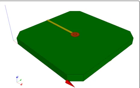
Fig. 1CAD model of a single via on a circuit board. Composite board (green) embeds a copper trace (yellow) and a thru hole via (brown)

a conductor and is embedded in the composite, which is an insulator. In order to set the ideas, consider Fig. 1. The board is clamped on the four chamfer faces. As in a real experiment, we can set the electric potential, φ in V(olt), on the ends of the via at front and back faces (onyz-planes) of the board. The electric potential differ-ence creates an electric field,Ei in V/m(eter), leading to

an electric current,Ji in A(mpere)/m2, measured on the

material frame. In other words, this current is the effective motion of charges with respect to the continuum body. Independently, the body can have a motion such as defor-mation, too. A deformation of the material is observed with respect to the laboratory frame. The electric current in the laboratory frame is given by

Ji=Ji+viρz, (1)

whereρdenotes the mass density in k(ilo)g(ram)/m3_,zthe specific charge in C(oulomb)/kg, andvithe velocity of the

continuum body as rate of displacement,vi =u•i. Strictly

speaking, the formulation is in the reference placement; however, by assuming small deformations we refrain from distinguishing between reference and current placement. Since the formulation is in the reference placement, the time rate (·)• is simply the partial time derivative. We search for the displacement, ui, effected by the electric

potential set on each end of the via. Concretely, we set one end zero (grounded); on the other end we apply a har-monic excitation with a relatively low frequency, thus, it is appropriate to presuppose that the magnetic potential is negligibly small,Ai =0, no magnetic flux emerges. Then

the electric field is given by the electric potential

Ei= −φ,i. (2)

A comma denotes a partial differentiation in space. The electric potentialφneeds to satisfy the balance of electric charge:

∂ρz

where and throughout the paper we understand the EINSTEIN summation convention over doubly repeated indices. We can reformulate the balance of electric charge. By using MAXWELL’s equation:

ρz=Di,i, (4)

with the charge potential (electric displacement) Di in

C/m2, we acquire

∂Di,i

∂t +Ji,i=0 . (5)

This governing equation will be used to compute the electric potential. Copper is a conductor so we can neglect its electric polarization. Composite board may exhibit an electric polarization, for the sake of brevity, we neglect this, too. We assume that both materials for the printed circuit board are unpolarized. We will discuss the connec-tion between charge potential, electric charge, and electric potential for unpolarized materials in the next section.

The electric current—flowing along the conducting trace and via—produces energy that alters temperature. Temperature distribution will be computed by satisfying the balance of entropy:

ρη•₊

i,i−ρ

r

T =, (6)

where the specific (per mass) entropy, η, its flux term, i, and its production term,, needs to be defined. The

entropy supply is given by the so-called radiant heat r, which is known. It is the term changing the temperature volumetrically, for example, in a microwave oven or in the case of a laser beam,ris the irradiated power of the oven or laser. For the printed circuit board, such a term is not supplied, r = 0. After a careful study for unpo-larized materials in (Abali 2016, Sect. 3.3), we know that we may select the entropy flux and define the entropy production as

i=

qi

T , = −

qi

T2T,i+ 1

TJiEi+

1

Tσij p_ε•

ij. (7)

Heat flux,qi, and stress,σij, will be defined in the next

section. The plastic strainpεijcomes from the small

defor-mation plasticity, where the the total strain is decomposed additively into a reversible as well as irreversible (plastic) part

εij= rεij+ pεij. (8)

By assuming small strains we can use the linear strain measure:

εij=

1 2

ui,j+uj,i

, (9)

whereuidenotes the displacement field to be computed.

Definition of the plastic strain will be given in the next section. Now we have found out the governing equation for the temperature,

ρ∂η ∂t +

_qi T

,i=. (10)

Initially the temperature is set at the so-calledreference

temperature of 300 K. Any deviation from the reference temperature induces a stress, which will be implemented via constitutive equations in the next section.

Induced stress causes a deformation. We search for dis-placements leading to that deformation. The stress,σji, is

the momentum flux in the balance of linear momentum:

ρv•_i −σji,j−ρfi=Fi, (11)

where the specific body force fi is given—gravitational

acceleration is a specific body force—and the production termFidefines the interaction with the electromagnetic

forces. For the application that we want to study, the grav-itational forces have a negligible effect, so we simplify the system by setting fi = 0. For unpolarized systems, the

production term is the LORENTZforce density:

Fi=ρzEi+(J×B)i=Dj,jEi, (12)

since we have assumed that the magnetic flux vanishes,

Bi = 0. The displacement has to fulfill the governing

equation:

ρ∂2ui

∂t2 −σji,j−Dj,jEi =0 . (13) We can computeφ,T, andui from Eqs. (5), (10), (13),

respectively, after having definedDi, Ji,qi, η, σij,pε•ij by

means ofφ,ui,T.

Constitutive equations

We aim at defining the charge potential Di, the

elec-tric current Ji, the heat flux qi, the specific entropy η,

the stressσij, and the rate of plastic strainpε_ij•. They are

called constitutive or material equations closing the gov-erning equations leading to partial differential equations of the electric potential φ, the displacementui, and the

temperatureT.

The necessary connection for the charge potential is given by the so-called MAXWELL–LORENTZ aether relation:

Di=ε0Ei, (14)

with the universal constantε0=8.85·10−12C/(V m). For the electric current we use OHM’s law:

where the electrical conductivity,ς, is a material depen-dent parameter. For the heat flux we use FOURIER’s law:

qi= −κT,i, (16)

with the material parameter κ called the thermal con-ductivity. The material parameters may depend on the temperature as well as electric field. Usually they are given as constants since such measurements are challenging. In order to define stress and entropy, we restrict the mate-rials being simple such that their material parameters are constants. Then we can acquire for the entropy

η=cln

T Tref.

+ 1

ραijσij, (17)

and for the stress HOOKE’s law with DUHAMEL– NEUMANNextension:

σij=Cijkl

εkl− pεkl− thεkl

, (18)

where the thermal strain reads th_ε

ij=αij(T−Tref.) . (19) The heat capacity c, coefficients of thermal expan-sion αij, components of stiffness tensor Cijkl are

assumed to be constant, otherwise the above material equations are not valid, for a thermodynamical deriva-tion of all aforemenderiva-tioned constitutive equaderiva-tions, see (Abali 2016, Sect. 3.3).

In time the solution will be in a discrete fashion, where trepresents the time step. In order to calculate current (unknown) plastic strain,pεij, by using the (known) plastic

strain from the last time step, pε_ij0, incrementally, p_ε

ij= pε0ij+tpε•ij, (20)

we use PRANDTL–REUSStheory with kinematic hardening

p_ε• mn= γ

σ0

|ij|−βij0

Cijkl

ε• kl− thεkl•

4 9hσY2+

σ0

|ij|−βij0

Cijkl

σ0

|kl|−βkl0 σ0

|mn|−βmn0

,

(21)

where the material parametershandσYare determined from a uniaxial tensile testing. The yield stress σY rep-resents the threshold for plastic deformation. The slope of stress versus plastic strain is given by h. The so-called MACAUL AYbrackets as inγdefines a conditional parameter as being 1 or 0 depending on theVONMISES equivalent stress,σeq, defined by the deviatoric stress,σ|ij|,

as follows

σeq=

2

3σ|ij|σ|ij|, σ|ij|=σij− 1

3σkkδij, (22) such that it becomes

γ = 1 ifσeq≥σY

0 otherwise . (23)

The so-called back stress,βij, evolves with the plastic

stress, again incrementally,

βij=βij0+tβij•, βij•= ¯cpεij•, (24)

where we are going to choosec¯=2h/3 in the simulations. A circuit board consist of copper traces and via embed-ded in a composite material. Since we want to detect the failure in the copper, we model the copper deforming elasto-plastically. Copper is a cubic material. In a circuit board copper has the thickness of 20–40μm whereas its grain size is only 0.5μm, see (Song et al. 2013). Hence we may assume that a polycristalline structure is present and the expected materials response is isotropic in this geometric scale. As a consequence of miniaturization this assumption may be critical in the near future. Hence we implement herein copper as a cubic material. For present-ing the difference between isotropic and cubic materials, consider an isotropic material with the following material parameter tensors

Cijkl =λδijδkl+μ

δikδjl+δilδjk

, αij=αδij, (25)

where the LAMEconstants,λ,μ, and the thermal expan-sion constant α are the necessary material parameters. The parameters, λ, μ, read from the engineering con-stants,E,ν,G, which can be measured directly:

λ= Eν

(1+ν)(1−2ν) = 2Gν

(1−2ν), μ=

E

2(1+ν) =G. (26)

YOUNG’s modulus, E, POISSON’s ratio, ν, and shear modulus,G, are coupled for isotropic materials as follows

G= E

2(1+ν). (27)

In the case of a cubic material the latter relation fails to hold such that the material possesses three independent parameters, namelyE,G, andνneed to be measured inde-pendently. We can write the stiffness tensor in a matrix notation

CIJ =

⎛ ⎜ ⎜ ⎜ ⎜ ⎜ ⎜ ⎝

C1111 C1122 C1133 C1123 C1113 C1112 C2211 C2222 C2233 C2223 C2213 C2212 C3311 C3322 C3333 C3323 C3313 C3312 C2311 C2322 C2333 C2323 C2313 C2312 C1311 C1322 C1333 C1323 C1313 C1312 C1211 C1222 C1233 C1223 C1213 C1212

⎞ ⎟ ⎟ ⎟ ⎟ ⎟ ⎟ ⎠ ,

called the VOIGTnotation and calculate it as the inverse of the compliance matrix,

CIJ =SJI−1 , SIJ =

⎛ ⎜ ⎜ ⎜ ⎜ ⎜ ⎜ ⎝ 1

E −Eν −νE 0 0 0

1

E −νE 0 0 0

1

E 0 0 0

1

G 0 0

sym. _G1 0 1 G ⎞ ⎟ ⎟ ⎟ ⎟ ⎟ ⎟ ⎠ . (29)

Analogously for the coefficients of thermal expansion

αij=

⎛

⎝ αx α0 0y 0

sym. αz

⎞

⎠ , (30)

we need to determine three independent coefficients for a cubic material. Necessary values for copper are taken from (Ledbetter and Naimon 1974, Table 10), (Deutsches Kupferinstitut 2014; Srikanth et al. 2007) as follows

C_IJCu= ⎛ ⎜ ⎜ ⎜ ⎜ ⎜ ⎜ ⎝

169.1 122.2 122.2 0 0 0 169.1 122.2 0 0 0 169.1 0 0 0 75.42 0 0

sym. 75.42 0

75.42 ⎞ ⎟ ⎟ ⎟ ⎟ ⎟ ⎟ ⎠

·109_{Pa ,}

αCu

ij =

⎛

⎝17 0 00 17 0 0 0 17

⎞

⎠_·10−6K−1,

σCu

Y =100·106Pa , hCu=615·106Pa ,

ρCu_=8.94·103_kg/m3_,

cCu=390 J/(kg K) , κCu=385 W/(K m) , ςCu_=5.8·107_{S/m .}

(31)

The composite material for the board is a fiber-reinforced laminate structure. Fibers are placed orthogo-nal in a woven structure such that the board material is orthotropic. For an orthotropic material, the compliance matrix in the VOIGTnotation reads

Sorth._IJ = ⎛ ⎜ ⎜ ⎜ ⎜ ⎜ ⎜ ⎜ ⎜ ⎝ 1

Ex −

νxy

Ey −

νxz

Ez 0 0 0

1

Ey −

νyz

Ez 0 0 0

1

Ez 0 0 0

1

Gyz 0 0

sym. _G1

zx 0 1 Gxy ⎞ ⎟ ⎟ ⎟ ⎟ ⎟ ⎟ ⎟ ⎟ ⎠ . (32)

All of 9 parameters need to be measured indepen-dently. Such a measurement is cumbersome. Instead, we can calculate the so-called homogenized parameters for the composite material. Consider different unidirectional plies stacked upon each other in such a way that we obtain an orthotropic material. In each unidirectional ply the material parameters can be calculated as a “weighted

sum.” A ply consists of fiber and matrix—parameters of fiber and matrix are easier to obtain separately. Therefore, first we determine the materials data of each unidirec-tional ply. Secondly, we sum the properties by considering a particular orientation leading to the orthotropic board.

A unidirectional ply is transverse-isotropic. In order to identify material parameters, we choose a coordinate system,(x1,x2,x3), where the first direction,x1, is along the fibers in the ply. With respect to this so-calledlocal

coordinate system, we obtain the following compliance matrix in the VOIGTnotation:

Sply_IJ = ⎛ ⎜ ⎜ ⎜ ⎜ ⎜ ⎜ ⎜ ⎝ 1

E11 − ν21

E11 − ν21

E11 0 0 0 1

E22 − ν23

E22 0 0 0 1

E22 0 0 0 2(1+ν23)

E22 0 0

sym. _G1

12 0 1 G12 ⎞ ⎟ ⎟ ⎟ ⎟ ⎟ ⎟ ⎟ ⎠ . (33)

These 5 parameters,E11,E22,ν21,ν23, andG12 can be calculated from the parameters of matrix and fiber by using micromechanical rules, see (Schürmann 2005,§8). These rules are simple models based on the linear elas-ticity. The most important assumption is that matrix and fiber be connected perfectly, in other words, no voids or cracks are existing such that the length change of matrix and fiber are identical. Then we can combine the mate-rials data of fiber and matrix; and we can calculate from them the parameters in a ply consisting of ϕ–fiber and (1−ϕ)–matrix as follows

E11 =ϕEf.11+(1−ϕ)Em.11 , E22= E m. 22E22f. ϕEm.

22+(1−ϕ)E22f. , ν21=ϕν21f. +(1−ϕ)ν21m.,

ν23 =ϕν23f. +(1−ϕ)ν23m. ⎛ ⎝ 1+ν

m. 23−ν21f.

Em.₁₁

Ef.₁₁

1−(νm. 23)

2_+νm. 23ν21f.

Em.₁₁

E₁₁f.

⎞ ⎠ ,

G12= G

m. 12Gf.12 ϕGm.₁₂+(1−ϕ)Gf.₁₂ ,

(34)

and

α

=

m.

11Em.11+ϕα11f.Ef.11 (1−ϕ)E11m.+ϕEf.11

,

α

=

ϕα

+(

1

−ϕ)α

,

α

=

ϕα

+(

1

−ϕ)α

.

(35)

Table 1Materials data of s-glass (I), e-glass (II), and aramid (III) fibers and epoxy matrix

S-glass (I) E-glass (II) Aramid (III) Epoxy Ply I Ply II Ply III

E11in GPa 85 65 100 4.2 53 41 62

E22in GPa 85 65 5.4 4.2 9.8 9.6 4.9

ν21 0.23 0.20 0.37∗ 0.34 0.27 0.26 0.36

ν23 0.4∗ 0.4∗ 0.4∗ 0.34 0.44 0.44 0.44

G12in GPa 33 28 1.5∗ 1.6 3.7 3.6 1.5

α11inμm/(m K) 1.5 4 –3 45 2.9 5.7 –2.2

α22inμm/(m K) 1.5 4 17 45 18.9 20.4 28.2

α33inμm/(m K) 1.5 4 17 45 18.9 20.4 28.2

Parameters marked with∗are approximated values

Calculated unidirectional plies with s-glass, e-glass, and aramid are denoted by Ply I, II, and III, respectively

parameters for a unidirectional ply, we can simply con-struct a laminate of several plies by stacking them orthog-onally. The result is an orthotropic material. Owing to the linear constitutive equations, we can superpose each ply’s material tensors as transformed to the global coor-dinate system. All necessary materials data are compiled in Table 2. In addition to the aforementioned materials parameter, we use for laminate the following data:

ρlam._{=2500 kg/m}3_{, c}lam._{=800 J/(kg K) ,}

κlam._{=1.3 W/(m K) , ς}lam._{=0 .} (36)

Weak form

The primitive variables,φ,ui,T, are continuous functions

in space and time. We want to compute them by satis-fying Eqs. (5), (13), (10) augmented by the constitutive equations introduced in the last section. We will approxi-mate space by means of finite element method (FEM) and

Table 2Materials data of Lam. I (s-glass and epoxy), Lam. II (e-glass and epoxy), and Lam. III (aramid and epoxy) in the global coordinate system

Lam. I Lam. II Lam. III

Exin GPa 32 25 34

Eyin GPa 32 25 34

Ezin GPa 11 11 6

νxy 0.09 0.10 0.05

νxz 0.14 0.16 0.08

νyz 0.14 0.16 0.08

Gyzin GPa 3.5 3.5 1.6

Gzxin GPa 3.5 3.5 1.6

Gxyin GPa 3.7 3.6 1.5

αxinμm/(m K) 10.9 13.1 13.0

αyinμm/(m K) 10.9 13.1 13.0

αzinμm/(m K) 18.9 20.4 28.2

time by using finite difference method (FDM). Time dis-cretization is quite intuitive, as a list of subsequent time steps, whereas for simplicity in programming we choose identical time steps

t= {0,t, 2t,. . .}. (37)

Instead of a partial time derivative, we write the follow-ing difference equations:

∂(·) ∂t =

(·)−(·)0

t ,

∂2_(·)

∂t2 =

(·)−2(·)0+(·)00 tt , (38)

where (·)0 and(·)00 indicate the computed values from the last and second last time steps, respectively. In order to approximate the functions in a discretized space, we multiply the governing equations by appropriate test func-tions and obtain a variational form for each primitive variable,

Fφ=

e

Di,i−D0i,i

t +Ji,i

δφ dV =0 ,

Fu=

e

ρui−2u0i +u00i

tt −σji,j−Dj,jEi

δui dV=0 ,

FT =

e

ρη−η0

t +i,i−

δT dV=0 ,

(39)

integrated over a finite elemente. The forms Fφ and FT

are in the unit of power, whereas Fuis in the unit of energy.

By multiplying Fφ and FT by t, we obtain all forms in

the same unit. The following terms:Di,Ji,σji,iconsist

by parts such that one of the derivatives is shifted to the corresponding test function, as follows

Fφ= −

e

Di−D0i +tJi

δφ,i dV

+

∂e

Di−D0i +tJi

δφNi dA,

Fu=

e

ρui−2u0i +u00i

tt δui+σjiδui,j −Dj,jEiδui

dV−

∂eσjiδ

uiNj dA,

FT=

e

ρη−η0_δT−t

iδT,i

−tδT)dV+

∂etiδTNi dA,

(40)

withNibeing the plane normal pointing outward frome.

The latter integral forms are called the weak forms. The whole computational domain,, consists of two different materials, each material is divided by finite elements sat-isfying F=0 with

F=F_φ+Fu+FT. (41)

We can assembly by summing over all elements. An ele-ment with its plane normal Ni and its adjacent element

with its opposing plane normal eliminate the boundary terms within a material. All primitive variables are contin-uous. Over the interface,∂I, between different materials, there may occur jumps since the material parameters have different values. The weak forms read

F_φ=−

Di−D0i +tJi

δφ,idV

+

∂IDi−D

0

i+tJiδφNi dA

+

∂

Di−D0i +tJiδφNidA,

Fu=

ρui−2u0i +u00i

tt δui+σjiδui,j−Dj,jEiδui

dV

−

∂IσjiδuiNj dA−

∂σjiδuiNj dA, FT =

ρη−η0_δT−t

iδT,i−tδT

dV

+

∂ItiδTNi dA+

∂tiδTNi dA. (42)

On the interface, i.e., between two different materials, sinceφ is continuous,Di is continuous, too. No electric

current is allowed along the normal direction, since cop-per is surrounded by the insulating board or air. Accord-ing NEW TON’s lemma—action is equal to reaction—we

expect that traction vectorsti = Njσji are also

continu-ous. On the boundary,∂, the traction vectorˆtiis given.

In our example, we have free surfaces such thatˆti= 0 on

∂or clamped faces where the displacement is given (as zero). On boundaries where the solution is given, we apply a DIRICHLET boundary condition and the test function vanishes. Temperature at the boundary can be modeled by using mixed boundary condition such that a devia-tion from the reference temperature causes a heat flux,

qiNi = ¯h(T−Tref.), depending on the convective heat transfer coefficienth¯ in J/(s m2K). Finally, we acquire the weak form to be implemented

F=

−Di−D0i

δφ,i−tJiδφ,i

+ρui−2u0i +u00i

tt δui+σjiδui,j−Dj,jEiδui +ρη−η0_δT−t

iδT,i−tδT

dV

+

∂ItiδTNi dA+

∂t ¯

h(T−Tref.)

δT T dA.

(43)

We exploit the open-source packages developed under the FEniCS project and solve the coupled and nonlinear weak form for the simulations demonstrated in the next sections.

Lifetime prediction

Under a cyclic loading, copper traces and via deform plas-tically and material fails after a number of cycles,Nf.. Since plastic deformation is irreversible, in each cycle, plastic deformation accumulates. By means of computation we can determine the accumulated plastic strain in one cycle and use this as a measure of lifetime. The plastic strain rate, pε•_ij, is deviatoric, thus, the equivalent strain rate reads

p_ε• eq.=

3 2

p_ε•

ijpεij•. (44)

The plastic strain accumulates in a cycle with the latter rate of equivalent strain,

p_ε acc.=

cycle p_ε•

eq.dt. (45)

This accumulated strain is a distribution in the copper wire. Its mean value can be determined by averaging over a chosen volumeV

_p ε=

Vpεacc.dV VdV

(46)

number of cycles to failure,Nf., there are various sugges-tions. They are mostly empirical such as computations and experiments need to be conducted and fitted. A the-oretical analysis in (Manson 1968) provides the following relation

p_{ε =D}0.6_N−0.6

f. , (47)

for metallic compounds such as copper used in traces and via. The material specific constant,D, reads from the reduction of cross section,R, in a tensile test,

D=ln

100 100−R

. (48)

Cross section reduction,R, is in percentage and we take it as R = 60 for the electrodeposited copper material, see (Valiev et al. 2002). It is important to recall that the parameter Dcan be obtained from a tensile testing. By employing computation we obtainpε and estimate the lifetime

Nf.=Dpε−5/3. (49)

This lifetime estimation is for the case of an acceler-ated test. It is challenging to determine a specific amount of months or years for the underlying electronic device. For comparing several designs, it is a helpful measure. A design with a longer lifetime is expected to be chosen from the point of mechanics.

Results and discussion

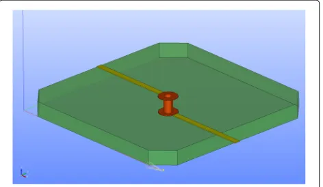
For analyzing the multiphysics and estimating the number of failure on a simplified unpopulated—so-called bare -board—we choose realistic geometric dimensions used in the industry. As shown in Fig. 2, the CAD geometry is pre-pared and preprocessed in Salome v7.5 (Salome 2017) by using NETGEN algorithms (Schöberl 1997). We have cho-sen a board of dimensions 10×10×0.8 mm. Although all material parameters are given in SI units, we have converted them into mm, Mg (tonne), s, mA, K for the

Fig. 2Simulation model of the one layer circuit board. Composite board (green,transparent) embeds a copper trace (yellow) and a thru hole via (brown)

simulation such that the geometry is captured accurately (up to the machine precision) in mm. The conducting wire is calledtraceandvia, both from the same material, namely 5N copper. We use a standard 1 oz. copper mod-eled with 35μm of thickness. Starting from the back side of the board, a trace alongx-axis is placed on top of the board. The trace has a width of 300μm and is connected by the annular ring (pad) of 500μm radius to the thru hole via. Trace and annular ring are produced by masking and etching. Actually the profile of the trace and ring is trape-zoidal due to the etching process; however, we model it as rectangular. After ring and trace are plated, a hole with 200μm radius is drilled and the via is electroplated with a given thickness. Herein we model the wall thickness of the via also as 35μm. There are no standards for this thickness and the simulation results would be different by varying this thickness. Via connects the trace on top to the trace on bottom that runs until the front side of the board. Espe-cially around traces and via, several refinements of the mesh are applied; the final finite element mesh can be seen in Fig. 3.

We present simulations of a possible measurement. All boundary conditions are selected as it would be the case in reality. Board is usually fastened by bolts on four holes near to the edges. In order to hold the board on four edges, we model chamfers on the edges and hold on these four chamfer faces as being clamped in all directions. We sim-ply set the deformation zero as a DIRICHLET boundary condition. The conducting copper is driven by an electric potential difference. At the endings of traces on back and front faces, the electric potential is set as a DIRICHLET boundary condition. One end is grounded and the other is given harmonically,

ˆ

φ=φamp.sin(2πνt). (50)

For all simulations we have selected the period of 10 s leading to the frequency ν = 0.1 Hz and an amplitude asφamp. = 0.2 V in order to reach high enough temper-atures leading to significant plastic strains. Since we have only a highly conductive copper wire, even such a small potential difference lead to high electric currents and dis-sipated heat, JOULE’s loss. This setting is also configured in an accelerated fatigue test; but in an electronic device such conditions are not valid. Normally, there is a compo-nent like a resistor or capacitor connected to the circuit such that the electrical conductivity is lowered, leading to a smaller current, thus, a lower temperature increase. The computational model mimics a possible accelerated active fatigue experiment. In order to simulate an existing test; geometry and boundary conditions need to be accurately determined and applied.

The weak form in Eq. (43) is nonlinear. By using FEniCS packages the linearization is handled automatically at the level of the partial differential level, before the assembly. Solution is searched by a standard NEW TON–RAPHSON algorithm after assembly operation. Every time step lasts approximately 8 min on one (3 min on two) Intel Xeon Processors (i7-2600) running on Ubuntu 16.04.

In order to comprehend the complicated multiphysics bearing electro-thermo-mechanical coupling, we present several results on one board at the quarter of one period,

t=2.5 s. The results with other laminates are qualitatively the same. The potential difference generates an electric current. It is in equal amount in ampere along the trace and via. The current density,Ji, is the amount per cross

section. Since we have chosen the trace as well as via of the same thickness and the circumference of the via is longer than the width of the trace, the current density is greater along the trace than through the via. The electric potential and current density can be seen in Fig. 4. Greater elec-tric current density implies a greater JOULE’s heat, JiEi,

directly responsible for the temperature increase. Hence,

Fig. 4Simulation results att=2.5 s, electric potential and current density. For the sake of visibility, electric potentialφand electric current densityJiare presented on the transparent copper conductor. Color distribution denotes the electric potential. Arrows indicate the current density

Fig. 5Simulation results att=2.5 s, temperature distribution. Temperature distribution,T, is shown as colors on the sliced model, the other half has a mirror symmetry

the temperature increase is more on the trace than on the via. The temperature distribution again at the quar-ter period can be depicted in Fig. 5. For another wall thickness, this result would be different.

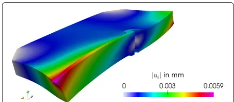
It is of importance to recall that the temperature distri-bution is not homogeneous, which is indeed the case in reality. This fact is overseen in an accelerated fatigue test performed in an oven. Temperature is changed quickly in the chamber, as a consequence, a homogeneous tem-perature distribution emerges, since the board is thin and copper is a good conductor. In this configuration the dam-age occurs in the via. In an active test, however, we realize that the temperature distribution is heterogeneous that lead to another deformation mode in each cycle. In order to visualize the deformation, see Fig. 6. It is interesting to see that the middle part of the via is not moving; how-ever, the variation of the displacement along the hole still induces a strain.

Approximately more than 20 K deviation from the reference temperature Tref. = 300 K results stresses higher than the yield stress and plastic deformation starts accumulating. Simultaneously, heat escapes to the ambi-ent, in the simulation we use the same convective heat transfer coefficients for the board as well as via, h¯ =

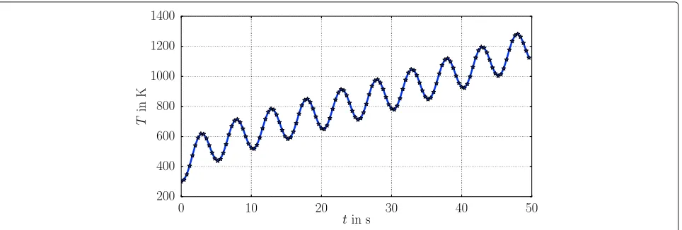
Fig. 7Temperature increase. Maximum temperature is presented over time for 5 cycles

10 J/(s m2K), modeling a relatively slow free convection. This parameter is very difficult to measure accurately such that we choose a value and use the same for all simulations.

Temperature is produced within the conductor and exchanged over its boundary at the same time. Change across the boundary is greater when the temperature on the boundary increases. However, since we model free convection, this rate is small compared to the heat pro-duction. Depending on the excitation frequency of the given electric potential and depending on the convective heat transfer coefficient, the temperature increases until the heat exchange rate and production are equal in their absolute values. This steady-state condition is difficult to reach in the simulation, at least for the first 5 cycles the steady-state is not reached, see Fig. 7. We realize that a real experiment with the aforementioned setting might be difficult since within one minute the melting temperature of the board would be reached. Either a forced convec-tion (using a fan) or a resistor connected to the circuit decreases the temperature increase. Although the increase is high, the total difference between the maximum and minimum temperature remains approximately the same in every cycle.

The fatigue failure occurs mostly because of the plas-tic strain accumulation. At the end of the first cycle, see the equivalent plastic strains in Fig. 8. The heterogeneous temperature distribution and the presented deformation lead to high plastic strains in the trace as well as in the via. This result is different compared to a fatigue exper-iment in an oven, where the most of the plastic strain accumulates within the via. Herein, in an active testing, we observe especially at the middle height of the via higher values than within the trace. For a better comparison we determine the mean values in two different volumes: over the traces and over the via. The accumulation of the mean value of the plastic strain averaged over these two regions

can be seen in Fig. 9. Due to the irreversible character, the plastic strain accumulates whenever the temperature is increasing and remains the same at the moment when the temperature is decreasing. In every cycle the amount of the newly accumulated plastic strain is compiled in Table 3. A steady-state cannot be reached before the temperature variation gets stabilized.

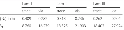
Results in all laminates are qualitatively similar. They do differ quantitatively in terms of the plastic strain. In order to compare different laminates and their effects to the fatigue behavior, we conduct three simulations and com-pute the mean accumulated plastic strain at the end of one cycle. Again the aforementioned two volumes are used for averaging. The choice of the averaging volume is some-how heuristic and challenging; some-however, for a comparison between three laminates, the choice fails to be relevant. The values are compiled in Table 4.

By considering the fatigue as the sole criterion, it is fair to claim that the laminate III—aramid reinforced epoxy composite material—performs better than glass fiber rein-forced epoxy materials. Since the governing equations are coupled and nonlinear, such a conclusion is chal-lenging to predict based on the material parameters.

Fig. 9Accumulated plastic strains. Accumulation of the plastic strains. Mean value over traces and via are presented for 5 cycles

Laminate III has the highest thermal expansion coeffi-cient along the plate thickness, so the mismatch between expansion coefficients is higher. Hence, it is intuitive to guess that it would lead to greater plastic strains. As we see from the deformation mode, the boundary con-ditions lead to a more shearing deformation that is the real reason of a plastic deformation. Expansion along the board thickness reduces shearing deformation lead-ing to smaller plastic strains. Based on only one of the material parameters, we might prejudge the outcome dif-ferently than the observation by means of computations as presented herein. There are many coupling effects act-ing simultaneously, the only prediction shall be based on simulations with the least number of assumptions. Herein we present a robust method for computing an electro-thermo-mechanical system. In order to verify the code, we need to simulate existing experiments by correctly choosing boundary conditions as well as the geometry. According to the demonstrated comparison, a different choice for the laminate composition might increase the fatigue strength. There is a growing attention to find out variations of FR4 PCBs out of e-glass and epoxy. Stablcor Technology Inc. has patented its own PCF consisting of carbon fibers. Thermount is a registered trademark by DuPont and it uses aramid fibers.

Table 3Mean accumulated plastic strain in each cycle for the laminate I

p_{εin %}

Cycle Trace Via

1 0.409 0.282

2 0.377 0.305

3 0.417 0.293

4 0.455 0.315

4 0.497 0.352

Coupled computations is of importance to obtain a detailed investigation guiding toward newer insight into multiphysics. Herein we have neglected magnetic poten-tial and thermoelectric effects. Often more assump-tions are undertaken in order to simplify or decouple the governing equations leading to a fast simulation. With today’s technological possibilities, we can perform computations as presented herein by using a laptop. Hence, we can get a detailed understanding of the phe-nomenon and even suggest design changes. In order to enable a scientific exchange, we deliver our codes in (Abali 2011) to be used under the GNU Public license (GNU Public 2017).

Conclusions

Using rational continuum mechanics, all necessary gov-erning equations and constitutive equations are pre-sented for an electro-thermo-mechanical system. We have directly attacked an application from electronics industry, namely a phenomenon called fatigue in cop-per vias. Accelerated excop-periments are generally con-ducted in an oven so the temperature is controlled glob-ally. In the recent years, more sophisticated experiments started to emerge, where the electric potential is con-trolled that leads to a local heating. This multiphysics problem is challenging to compute numerically, since the governing equations are nonlinear and coupled. We have presented an approach for computing coupled and

Table 4Number of failure calculated by the accumulated plastic strain in each cycle for three different laminates

Lam. I Lam. II Lam. III

trace via trace via trace via

p_{εin % 0.409 0.282 0.318 0.236 0.262 0.204}

nonlinear governing equations by means of open-source packages and simulated the electro-thermo-mechanical system monolithically. The results seem to be promising, a verification with experimental results is left to future research.

Abbreviations

FDM: Finite difference method; FEM: Finite element method; PCB: Printed circuit board

Acknowledgements

This work was completed while B. E. Abali was supported by a grant from the Max Kade Foundation to the University of California, Berkeley.

Funding

This work was completed while B. E. Abali was supported by a grant from the Max Kade Foundation to the University of California, Berkeley.

Availability of data and materials

All codes used for simulations are publicly available in (Abali 2011) licensed under the GNU Public license (GNU Public 2017).

Competing interests

The author declares that he/she has no competing interests.

Publisher’s Note

Springer Nature remains neutral with regard to jurisdictional claims in published maps and institutional affiliations.

Received: 14 December 2016 Accepted: 24 April 2017

References

Abali BE (2011) Technical University of Berlin, Institute of Mechanics, Chair of Continuums Mechanics and Material Theory, Computational Reality. http://www.lkm.tu-berlin.de/ComputationalReality/

Abali BE, Reich FA, Müller WH (2014a) Fatigue analysis of anisotropic copper-vias in a circuit board. GMM, Mikro-Nano-Integration. VDE Verlag, Berlin

Abali BE, Lofink P, Müller WH (2014b) Variation of plastic materials data of copper and its impact on the durability of Cu-via interconnects. In: Aschenbrenner R, Schneider-Ramelow M (eds). Microelectronic Packaging in the 21st Century. Fraunhofer Verlag. pp 305–308. Chap. 7.2

Abali BE (2016) Computational Reality, Solving Nonlinear and Coupled Problems in Continuum Mechanics. Advanced Structured Materials. Springer, Singapore

Alnaes MS, Mardal KA (2012). In: Logg A, Mardal K-A, Wells GN (eds). Automated solution of differential equations by the finite element method, the FEniCS book. Springer. Chap. 15 Syfi and sfc: symbolic finite elements and form compilation

Atli-Veltin B, Ling H, Zhao S, Noijen S, Caers J, Weifeng L, Feng G, Yuming Y (2012) Thermo-mechanical investigation of the reliability of embedded components in pcbs during processing and under bending loading. In: Thermal, Mechanical and Multi-Physics Simulation and Experiments in Microelectronics and Microsystems (EuroSimE), 2012 13th International Conference On. IEEE. pp 1–4

Deutsches Kupferinstitut (2014) Kupfer in der Elektrotechnik – Kabel und Leitungen. www.kupferinstitut.de

FEniCS project (2017) Development of tools for automated scientific computing:2001–2016. http://fenicsproject.org

GNU Public (2017) Gnu general public license. http://www.gnu.org/copyleft/ gpl.html

JPS Industries Inc. Company JPS Composite Materials (2017). http://jpsglass. com/jps_databook.pdf

Kpobie W, Martiny M, Mercier S, Lechleiter F, Bodin L, des Etangs-Levallois AL, Brizoux M (2016) Thermo-mechanical simulation of pcb with embedded components. Microelectron Reliab 65:108–130

Ledbetter H, Naimon E (1974) Elastic properties of metals and alloys. ii. copper. J Phys Chem Ref Data 3(4):897–935

Manson S (1968) A simple procedure for estimating high-temperature low-cycle fatigue. Exp Mech 8(8):349–355

Ridout S, Bailey C (2007) Review of methods to predict solder joint reliability under thermo-mechanical cycling. Fatigue Fract Eng Mater Struct 30(5):400–412

Roellig M, Dudek R, Wiese S, Boehme B, Wunderle B, Wolter KJ, Michel B (2007) Fatigue analysis of miniaturized lead-free solder contacts based on a novel test concept. Microelectron Reliab 47(2):187–195

Salome (2017) The Open Source Integration Platform for Numerical Simulation. http://www.salome-platform.org

Schürmann H (2005) Konstruieren Mit Faser-Kunststoff-Verbunden. Springer, Berlin

Schöberl J (1997) NETGEN an advancing front 2d/3d-mesh generator based on abstract rules. Comput Vis Sci 1(1):41–52

Solomon HD (1991) Predicting thermal and mechanical fatigue lives from isothermal low cycle data. In: Solder Joint Reliability. Springer. pp 406–454 Song JM, Wang DS, Yeh CH, Lu WC, Tsou YS, Lin SC (2013) Texture and

temperature dependence on the mechanical characteristics of copper electrodeposits. Mater Sci Eng A 559:655–664

Soden P, Hinton M, Kaddour A (1998) Lamina properties, lay-up configurations and loading conditions for a range of fibre-reinforced composite laminates. Compos Sci Technol 58(7):1011–1022

Srikanth N, Premkumar J, Sivakumar M, Wong Y, Vath C (2007) Effect of wire purity on copper wire bonding. In: Electronics Packaging Technology Conference, 2007. EPTC 2007. 9th. IEEE. pp 755–759

Suter Kunststoffe AG (2017). http://www.swiss-composite.ch/pdf/i-Werkstoffdaten.pdf

Valiev R, Alexandrov I, Zhu Y, Lowe T (2002) Paradox of strength and ductility in metals processed bysevere plastic deformation. J Mater Res 17(01):5–8

Submit your manuscript to a

journal and benefi t from:

7Convenient online submission 7Rigorous peer review

7Immediate publication on acceptance 7Open access: articles freely available online 7High visibility within the fi eld

7Retaining the copyright to your article