Super-resolution via a fast deconvolution with kernel estimation

R E S E A R C H

Open Access

Super-resolution via a fast deconvolution

with kernel estimation

Han Yu, Ting-Zhu Huang

, Liang-Jian Deng and Xi-Le Zhao

Abstract

Image super-resolution has wide applications in biomedical imaging, computer vision, image recognition, etc. In this paper, we present a fast single-image super-resolution method based on deconvolution strategy. The deconvolution process is implemented via a fast total variation deconvolution (FTVd) method that runs very fast. In particular, due to the inaccuracy of kernel, we utilize an iterative strategy to correct the kernel. The experimental results show that the proposed method can improve image resolution effectively and pick up more image structures. In addition, the speed of the proposed method is fast.

Keywords: Super-resolution, Kernel estimation, Fast total variation deconvolution (FTVd)

1 Introduction

The process of estimating a high-resolution (HR) image from one or multiple low-resolution (LR) images is often referred to as image super-resolution. According to the number of low-resolution images, image super-resolution can be divided into two categories: one is single-image resolution, and the other is multiple-image super-resolution. Based on image sequence, multiple-image super-resolution uses overlapping information between multiple low-resolution images to estimate details of the high-resolution image [1–3]. Due to multiple-image super-resolution needs more than one input image, it cannot deal with the situation when only one image is inputted. In this paper, we mainly focus on single-image super-resolution.

Interpolation-based methods are one of classical image super-resolution methods. To determine pixel values of each position in the high-resolution image, interpolation-based methods need to construct a rational interpolation function. The conventional interpolation-based meth-ods contain bicubic interpolation method, cubic inter-polation method [4], cubic spline interinter-polation method, nearest-neighbor interpolation method, etc. These meth-ods usually run very fast but always produce blurring or jagged artifacts. Recently, many contributions in terms of

*Correspondence: [email protected]

Research Center for Image and Vision Computing/School of Mathematical Sciences, University of Electronic Science and Technology of China, Xiyuan Ave, 611731 Chengdu, China

interpolation-based methods have been proposed [5–11]. In [6], Zhang et al. present an edge-guided interpolation algorithm through directional filtering and data fusion. This method can preserve sharp edges. In [9], Wang et al. propose a fast image upsampling method within a two-scale framework. They use interpolation method to recover the low-frequency image and reconstruction technique to recover the local high-frequency structures.

Reconstruction-based methods are another class of image super-resolution approaches. Through studying the low-resolution image generating process, reconstruction-based methods use a certain model to depict the map-ping relationship between the high-resolution image and the low-resolution image. There are three main types of reconstruction-based methods: frequency domain tech-niques, spatial domain techtech-niques, and other techniques. Frequency domain techniques [12–14] solve the problem in frequency domain, and the observation model is based on displacement characteristics of Fourier transform. Spa-tial domain techniques, such as non-uniform interpola-tion within samples method [15], convex set projecinterpola-tion method [16], statistical recovery method (maximum a posteriori and maximum likelihood estimation) [2, 17, 18], solve the problem in spatial domain. In addition, there are some other reconstruction-based methods [19–24]. In [22], Shan et al. propose an efficient upsampling method which lies in a feedback-control framework. This method runs very fast and can preserve the essential structural information.

Learning-based methods are the third category of image super-resolution methods. Learning-based methods [25–32] need to train two dictionaries for low-resolution and high-resolution images or patches. When given a low-resolution image, learning-based methods can get a high-resolution image through using the learnt mapping relationship between the two dictionaries. Although these methods obtain good visual results, they rely on the two training dictionaries and cannot change the magnification factor arbitrarily.

In this paper, we propose a new single image super-resolution method based on deconvolution strategy. According to Efrat et al. [33], an accurate kernel is more important than a sophisticated prior for image super-resolution. Thus, we take into account the error of blur kernel in our method. We develop an iterative strategy to adjust the blur kernel and then estimate the final high-resolution image via a reconstruction method. The proposed method is based on the framework of [22]. How-ever, it has two main contributions. First, the proposed method can get faster speed than [22], since we employ a fast total variation deconvolution (FTVd) method in our work. Second, the proposed method estimates the deconvolution kernel iteratively to get better visual and quantitative results than [22].

The rest of this paper is organized as follows. Section 2 introduces image super-resolution problem, reviews FTVd method and a fast image upsampling method. In Section 3, we detail the proposed model and algorithm. Numerical results are shown in Section 4. Finally, we draw some conclusions in Section 5.

2 Problem description and related works 2.1 Image super-resolution problem

LetHbe a high-resolution image and letf be the camera’s point spread function (PSF) which is approximated by a Gaussian filter. According to [1], the low-resolution image can be modeled as

L=f ⊗H↓d, (1)

where↓dis a downsampling operator with factord. This equation can be broken down into two steps,

B=f ⊗H,L=B↓d, (2)

whereBis a linearly filtered high-resolution image. Image super-resolution is to recover the high-resolution imageH from an input low-resolution imageL.

2.2 Image super-resolution problem

FTVd method is a popular way to solve the problem of image restoration [34]. Image restoration is a process of recovering images from blurring and noise observation. This process can be modeled as

g=Au+n, (3)

where g represents the observed image, A represents a convolution matrix,uis an original image, andnis ran-dom noise.

A degraded imageucan be recovered from the following simple model:

min

u

i

Diu +μ

2Au−g 2

2, (4)

whereDiuis the discrete gradient ofuat pixeli,iDiu

is the discrete total variation (TV) ofu, andμis a regular-ization parameter.

Actually, similar cases with the above problems have been studied by many works [34–39]. In particular, FTVd method [34] is one of effective methods for solving Eq. (4). In [34], Wang et al. utilize an auxiliary variablewi to

substituteDiuto generate the following problem:

min w,u

i

wi2+β 2

i

wi−Diu22+ μ

2Au−g 2 2, (5)

whereβis a penalty parameter.

This model is a half-quadratic model, which can be applied to total variation discretization with anisotropic or isotropic form. In [34], Wang et al. use a fast total variation deconvolution (FTVd) method to solve Eq. (5) (see Algorithm 1). This algorithm can be applied to image deblurring with different blurring kernels and different noise.

Algorithm 1 Fast total variation deconvolution (FTVd) method

Input:g,A,μ >0,β0>0 andβmax> β0.

Output:wandu.

Initialize:u=g,β=β0

whileβ ≤βmaxdo

while“ not converged "do Step 1: Computingwby

wi=max

Diu −

1 β, 0

Diu

Diu

; (6)

Step 2: Solvinguvia

i

DT_i Di+μ_βATA u=

i

DT_i wi+μ_βATg;

(7)

Note that Eq. (7) can be solved by Fast Fourier transforms (see more details in [34]).

end while

Step 3: Computingβby

β=2β; (8)

2.3 Fast image upsampling method

In [22], Shan et al. introduce a new single image super-resolution method. This method can enhance image res-olution automatically and preserve essential structural information. A key feature of this method is a feedback-control framework that contains three parts: deconvolu-tion, reconvoludeconvolu-tion, and pixel substitution.

In the deconvolution process, Shan et al. [22] take a non-blind deconvolution method. The non-blind decon-volution method is to solve the following energy function:

E(H)∝f⊗H−B2₂+λ((∂xH)1+ (∂yH)1), (9)

where∂xH and∂yH are the values of thexandy

direc-tion gradients, respectively.λ is a regularization param-eter. After the deconvolution process, the output image is refiltered in the reconvolution stage. In the process of pixel substitution, pixels of the low-resolution image are utilized to replace the pixels at the corresponding locations of the high-resolution image. There are two advantages for using pixel substitution. First, it can utilize the accurate low-resolution image pixels. Second, it can approximate the image, output from the reconvolution process, as a Gaussian-filtered image with a feedback-control loop. This method does not depend on the quality and quantity of the selected examples. Besides, the run-ning time of this method is very fast.

3 The proposed method 3.1 The proposed framework

In this section, we give the proposed method which is con-sisted of four parts: deconvolution, estimating blur kernel, reconvolution, and pixel substitution.

Figure 1 shows the diagram of our framework. In our scheme, the input is a low-resolution image L. We first transform the low-resolution image from RGB color space to YUV color space. Next, we upsample the low-resolution image to an ideal size by bicubic interpolation method and only conduct at Y space. We take an iterative strategy to achieve the image upsampling process (see Algorithm 2). Our strategy contains four parts: deconvolution, estimat-ing blur kernel, reconvolution, and pixel substitution. We take deconvolution process to eliminate the effect of the linear filtering. For instance, there are some visual arti-facts around the image “wheel” after bicubic interpolation in the Y space (see Fig. 1). Besides, because the accu-rate blur kernel can not be known exactly, the further estimated high-resolution image will become more inac-curate. Thus, we take account of the error of blur kernel. Furthermore, the same as [22], we take reconvolution and pixel substitution process to control the image upsam-pling. By applying our strategy iteratively at the initial

high-resolution image B(0)_{, we can obtained the} esti-mated high-resolution image at Y space. The final estimated high-resolution imageH∗is acquired by trans-forming the high-resolution image from YUV color space to RGB color space. We will show more details about the four steps of the proposed method (deconvolution, esti-mating blur kernel, reconvolution, and pixel substitution) as follows.

Algorithm 2 Single image super-resolution via a fast deconvolution with kernel estimation (see the flow chart of the framework from Fig. 1)

Input: a low-resolution image:L, upsampling factor:d, iteration number:τ, an initial kernel:f˜(0), regularization parameter:α.

Output: the high-resolution image:H∗.

Step 1: Getting the initial high-resolution imageB(0)by bicubic interpolation with the upsampling factord:

B(0)=Bicubic(L,d);

Step 2: Computing the estimating high-resolution imageH(i)_:

fori=1 :τdo

a. Computing the high-resolution image by FTVd method (see Algorithm 1):

H(i)=FTVd(B(i−1),f˜(i−1));

whereH(i)is equal tou,B(i−1)is equivalent togand the blur kernelf˜(i−1)can generateAin Algorithm 1. b. Estimating the error of blur kernele(i)via Eq. (11):

e(i)=Estimate(H(i),B(0),˜f(i−1),α);

whereH(i)is the intermediate high-resolution image andf˜(i−1)is the estimated blur kernel.

c. Updating the blur kernel:f˜(i)= ˜f(i−1)+e(i); d. Reconvoluting the imageH(i) by the initial kernel ˜

f(0):

Reblur= ˜f(0)_⊗H(i)_;

e. Updating the initial high-resolution image by pixel substitution (see details in Section 3.1):

B(i)=pixelsubs(L,Reblur);

end for

Step 3: Computing the final high-resolution image H∗=H(i).

3.1.1 Deconvolution

Let B(i) as a high-resolution that is gotten at iteration i,i ≥ 0, and B(0) is obtained by bicubic interpolation method. In particular,B(0) is obtained by bicubic inter-polation method. The deconvolution process, estimating the high-resolution imageH(i)_{, can be regarded as solving}

Fig. 1The flow chart of our framework. The low-resolution imageLis transformed from RGB color space to YUV color space. The proposed method includes four steps (deconvolution, estimating blur kernel, reconvolution, and pixel substitution) and is only applied to Y channel. The final resultH∗

is obtained via transforming the high-resolution image from YUV color space to RGB color space

multiplication ofWandH. Note that the problem of min-imizingf ⊗H−B2₂is hard to solve because the inverse ofWdoes not always exist and sometimesWcan be influ-enced by noise. In particular, taking the high-resolution image B as a blurred image, the deconvolution process can be considered as an image restoration problem. In this paper, we take FTVd method [34] in the deconvolution process, since FTVd method [34] is an effective way to deal with image restoration problem. The main steps of FTVd method are shown in Section 2.1.

3.1.2 Estimating blur kernel

Because the blur kernel is not known exactly in the image formation process, it may have some errors: f = ˜f +e, where f is the accurate blur kernel and f˜ is the inaccu-rate blur kernel containing an errore. In order to get a

reasonable high-resolution image, we need to consider the error of blur kernel.

We use the method similar to that described in [40] to estimate the blur kernel. Considering a connected

bounded domain ∈ R2 with compact Lipschitz

boundary, we take the initial high-resolution imageB(0), acquired by bicubic interpolation, as a blurred image and the intermediate high-resolution image atitimesH(i)as a real image.f˜be the blur kernel andebe the error of blur kernel. We study the following objective function to get the error of blur kernele:

min

e

˜

f +e⊗H−B2dx+α

e

2_{dx, (10)}

Table 1Parameter selection in terms of blur kernel and regularization parameter (case 1 is for the low-resolution image without ground truth; case 2 is for the low-resolution images acquired by downsampling the ground truth images)

Upscale factor Size Deviation _α

Case 1 2 5_×5 1.25 103

3 7×7 1.85 104

4 9×9 2.5 105

Case 2 2 3×3 1.5 103

3 5×5 1.8 104

4 7×7 2.3 105

whereαis a positive regularization parameter. This prob-lem can be solved by fast Fourier transform:

e=F−1

F−1_{(H)F(B− ˜f ⊗H)}

F−1_(H)F(H)+α , (11)

where F and F−1 _{are the Fourier transform and the} inverse Fourier transform, respectively. When we com-pute the errore, then the blur kernel can be estimated by f = ˜f +e.

3.1.3 Reconvolution

Taking account of reconvoluting the output image H(i) with the blur kernelf˜, the result should be close toB(i−1), wherei≥1. If not, there must be some incorrect pixel val-ues inB. So we need to modify the high-resolution image using the low-resolution image information, which leads

to pixel substitution in the next step. In particular, in each reconvolution step, we choose the initial blur kernelf˜(0) to reconvolute the high-resolution image. If we choose the updated blur kernel in the reconvolution process, the high-resolution image cannot be well estimated due to the change of blur kernel.

In the pixel decimation process, a low-resolution image is acquired by subsampling the high-resolution image with a downsampling factor d. In addition, the subsampling process only keep one pixel in the high-resolution image. Thus, the corresponding pixels in the high-resolution image can be substituted for pixels in the low-resolution image. In this paper, we take the pixel substitution strategy the same as [22] (see Fig. 2). If we upscale the low-resolution image fordtimes, we use the pixel(i,j)in the low-resolution imageLto replace the pixel(d×i+1,d× j+1)in the corresponding high-resolution imageReblur. Then, we can use the pixel-replaced image to conduct the next iteration. After several iterations, the estimated high-resolution imageH∗can be obtained. Our algorithm is given in Algorithm 2.

3.2 The difference between [22] and the proposed method

In [22], Shan et al. introduce a fast image/video upsam-pling method that involves a feedback-control frame-work. In particular, the proposed method has the similar feedback-control framework with the work in [22] (see Fig. 1). However, there are two main differences compar-ing with [22].

First, there are two different methods between [22] and the proposed method in the deconvolution process. Shan et al. [22] take account of a density distribution prior.

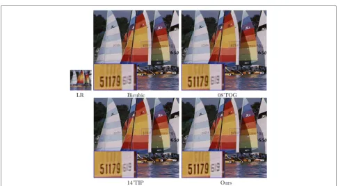
Fig. 4Visual results of “yacht” with the upsampling factor of 4. Fromlefttorightand then fromtoptobottom: the low-resolution image “yacht,” bicubic result, “08’TOG” [22], “14’TIP” [9], and our result

However, the proposed method utilizes FTVd method in the deconvolution process. Since the main step of FTVd method is fast Fourier transforms (FFTs) for each itera-tion, we can control the iterative number to get the faster speed and more accurate results than the decovolution method in [22].

Second, due to the inaccuracy of blur kernel in the deconvolution process, we employ a strategy of iterative kernel estimation to get more accurate kernel, aiming to make the resulted high-resolution image better. In con-trast, Shan et al. [22] only utilize a fixed Gaussian ker-nel. However, the fixed kernel cannot get better results obviously.

Table 2Times of test images (unit: seconds)

Example(factor) Bicubic 08’TOG [22] 14’TIP [9] Ours

Flower(4) 0.063 8.268 0.641 4.512

Yacht(4) 0.145 74.948 3.919 29.716

Wheel(3) 0.052 3.886 0.323 3.529

Comic(3) 0.073 17.136 1.281 5.654

Chilies(3) 0.032 8.053 0.466 3.403

Number(3) 0.055 5.518 0.416 4.255

House(2) 0.069 14.267 0.598 5.472

Starfish(2) 0.072 13.289 0.665 5.706

4 Numerical experiments

In this section, we test the proposed method on two kinds of images. One is the low-resolution images without ground truth, and the other is the low-resolution images acquired by downsampling the ground truth images. All experiments are conducted in MATLAB(R2010a) on a laptop of 3.47 GB RAM and Intel(R) Core(TM) i3-2130M CPU: @3.40 GHz.

We make comparisons between the proposed method and some state-of-the-art image super-resolution meth-ods, including bicubic interpolation, a fast upsampling method (“08’TOG” [22]1_{), a two-scale method (“14’TIP”} [9] 2_{) and two state-of-the-art interpolation methods} (“11’IPOL” [7]3and “11’SIAM” [8]4).

For grayscale image, we apply the proposed algorithm directly. For colored image, we first transform the low-resolution image to YUV color space and then only con-duct our algorithm on the Y channel. Images on the U and V channels are upsampled by bicubic method. After acquiring final upsampling image, we transform them from YUV space to RGB space for visual comparisons.

Fig. 5Visual results of “wheel” with the upsampling factor of 3. Fromtoptobottomand fromlefttoright: the low-resolution image “wheel,” bicubic result, “08’TOG” [22], “11’IPOL” [7], “11’SIAM” [8], “14’TIP” [9], and our result

favorite ways for determining parameters. Thus, we select parameters empirically in our experiments. For the size and the deviation of blur kernel, the regularization param-eterα, we fix them according to different kinds of test images and different values of the upsampling factor (see details at Table 1). In particular, we use the Gaussian ker-nel similar to that described in “08’TOG” [22]. In addition, we estimate the errors on many images with different iter-ation numbers, and find that two or three iteriter-ations can get the best results. In particular, we set the iteration number τas 2 in all experiments to reduce the computation time.

4.1 Results on the low-resolution images without ground truth

In this section, test images are the low-resolution images without ground truth; thus, it is not available to make quantitative comparisons. We compare the proposed method with bicubic interpolation method, “08’TOG” [22], “11’IPOL” [7], “11’SIAM” [8], and “14’TIP” [9]. The upsampling factors are 2, 3, and 4. In particular, if the dimensions of the estimated high-resolution images acquired by “11’IPOL” [7] and “11’SIAM” [8] exceed 800× 800, the images will be cropped. Hence, we do not show these results in Fig. 4, Fig. 6, Fig. 9, and Fig. 10 for the consistency of results.

In Figs. 3 and 4, we test the proposed method on the image “flower” and “yacht.” The upsampling factor is 4. From Fig. 3, the results of bicubic interpolation, “11’IPOL” and “11’SIAM” show significant blur effects along the image edge. Although the result by "08’TOG" preserves sharp edges, its luminance is not good enough for visual effects. As shown in this figure, our result can generate sharp edges, while enjoying a better effect of brightness. From Fig. 4, the number of our result is clearer than other results. In addition, after upsampling the image “yacht” with the factor of 4, the resolution comes to 2048×1920. However, this procedure only takes less than 30 s (see

Table 2). It demonstrates that the proposed method can deal with large-scale image resolution problem effectively. Figures 5, 6, 7 and 8 shows four example images with the upsampling factor of 3. In Fig. 5, there are some blur in the result of bicubic method and some staircases in the result of “08’TOG.” In the results of “11’IPOL” and “11’SIAM,” there are some visual artifacts. Despite preserving sharp edges and enjoying fast running time,

Fig. 6Visual results of “comic” with the upsampling factor of 3. From

Fig. 7Visual results of “chilies” with the upsampling factor of 3. Fromtoptobottomand fromlefttoright: the low-resolution image “chilies,” bicubic result, “08’TOG” [22], “11’IPOL” [7], “11’SIAM” [8], “14’TIP” [9], and our result

Fig. 8Visual results of “number” with the upsampling factor of 3. Fromtoptobottomand fromlefttoright: the low-resolution image “number,” bicubic result, “08’TOG” [22], “11’IPOL” [7], “11’SIAM” [8], “14’TIP” [9], and our result

Fig. 10Visual results of “starfish” with the upsampling factor of 2. Fromtoptobottomand fromlefttoright: the low-resolution image “starfish”, bicubic result, “08’TOG” [22], “14’TIP” [9], and our result

the result of “14’TIP” makes the image over-flat. How-ever, our result is able to introduce a better visual result. From Fig. 6, the proposed method provides sharp edges (see headdress and the green background). From Fig. 7, the result of the proposed method performs sharper edges than the results of bicubic method, “08’TOG,” and “11’IPOL”. In Fig. 8, the results of bicubic method, “08’TOG”, “11’IPOL,” and “11’SIAM” show blur effects sig-nificantly in the high-resolution images. For the result of “14’TIP,” it presents a clear high-resolution image but introduces significant staircases. In particular, the pro-posed method performs the best visual result comparing to other methods. Furthermore, the proposed method is faster than “08’TOG.” For instance, for the image “comic,” “08’TOG” requires 17.136 s, while the proposed method only needs 5.654 s (see Table 2).

In Figs. 9 and 10, we test our method on images “house” and “starfish” with the upsampling factor of 2. As shown in these figures, the proposed method preserves sharp edges and keeps more details. In addition, the running

time of our method is also much faster than “08’TOG.” For instance, for the image “starfish,” “08’TOG” needs 13.289 s, but our method only need 5.706 s to complete the image upsampling procedure (see Table 2).

4.2 Results on the low-resolution images acquired by downsampling the ground truth images

In this section, the low-resolution images are acquired by downsampling the ground truth images. We provide quantitative comparisons including root-mean-square error (RMSE), peak signal-noise ratio (PSNR), and struc-ture similarity (SSIM) [41].

We mainly compare the proposed method with one reconstruction-based method “08’TOG” and four interpolation-based methods, including bicubic method, “11’IPOL,” “11’SIAM,” and “14’TIP.” In Fig. 11, the test image is “castle” and the upsampling factor is 3. Note that the results of bicubic method and “08’TOG” present blur effects. The results of “11’IPOL” and “11’SIAM” show

Table 3Quantitative comparison in terms of RMSE, PSNR and SSIM

Example(factor) Index Bicubic 08’TOG [22] 11’IPOL [7] 11’SIAM [8] 14’TIP [9] Ours

House(2) RMSE 6.4742 6.0985 5.4645 5.3947 7.4008 5.1384

PSNR 31.9071 32.4263 33.3798 33.4915 30.7452 33.9143

SSIM 0.8831 0.8858 0.8961 0.8969 0.8761 0.8958

House(3) RMSE 8.9995 7.2818 7.8816 7.8106 9.1071 7.1034

PSNR 29.0465 30.886 30.1985 30.2771 28.9432 31.1015

SSIM 0.847 0.8655 0.861 0.8615 0.8554 0.872

House(4) RMSE 11.018 9.1549 9.8511 9.7658 11.7308 9.0703

PSNR 27.2887 28.8977 28.2611 28.3366 26.7443 28.9784

SSIM 0.8169 0.8418 0.8302 0.8311 0.8278 0.8444

Race(2) RMSE 11.18 11.2381 10.3093 10.1244 12.5453 10.8124

PSNR 27.1619 27.1169 27.8662 28.0234 26.1612 27.4524

SSIM 0.6912 0.6911 0.7353 0.7386 0.6536 0.692

Race(3) RMSE 13.9661 13.0151 13.0624 12.9765 14.1891 13.1136

PSNR 25.2293 25.8418 25.8103 25.8676 25.0917 25.7764

SSIM 0.6042 0.6078 0.6407 0.6429 0.5955 0.6171

Race(4) RMSE 15.7714 14.6136 14.8819 14.8098 15.7557 14.6909

PSNR 24.1734 24.8357 24.6776 24.7198 24.182 24.7898

SSIM 0.5524 0.562 0.5804 0.5826 0.5575 0.5761

some visual artifacts. Although the result of “14’TIP” can generate sharp edges, it has worse quantitative results (see Table 3). Furthermore, in this example, the proposed method shows the best RMSE, PSNR, and SSIM.

Figure 12 exhibits the results of image “race” with the upsampling factor of 2. From this figure, we can see that the results of bicubic method and “08’TOG” show some blur effects. The results of “11’IPOL” and “11’SIAM” introduce some artificial contours. The result of “14’TIP” exhibits sharp edges but smoothens the image details. The proposed method provides sharp edges and enjoys com-petitive quantitative results. More quantitative results are shown in Table 3.

5 Conclusions

In this paper, we presented a simple and effective sin-gle image super-resolution method. Our method was motivated by a fast image upsampling method, but we differently studied the estimated error of the blur ker-nel in the proposed method. We believed that the point spread function is not known exactly in the process of image super-resolution. Through applying a fast total vari-ation deconvolution (FTVd) strategy, we took an itera-tive updating strategy to update the blur kernel and the high-resolution image. In particular, the proposed method could be applied to any upscaling factors without any extra datasets. In addition, we analyzed the parameter

selection and computation time. Extensive experiments were provided to illustrate the effectiveness of the pro-posed method. Endnotes 1_{http://www.cse.cuhk.edu.hk/~leojia/projects/} upsampling/index.html. 2_{http://www.escience.cn/people/LingfengWang/} publication.html. 3_{http://demo.ipol.im/demo/g_image_interpolation_} with_contour_stencils/. 4_{http://demo.ipol.im/demo/g_interpolation_} geometric_contour_stencils/. Competing interests

The authors declare that they have no competing interests.

Authors’ contributions

HY performed the main part of this manuscript. TZH modified the content of the manuscript. LJD carried out the numerical results, and XLZ participated in the discussion. All authors read and approved the final manuscript.

Acknowledgements

This research is supported by 973 Program (2013CB329404), NSFC (61370147, 61170311), the Fundamental Research Funds for the Central Universities (ZYGX2013Z005).

Received: 27 September 2015 Accepted: 11 July 2016

References

1. S Baker, T Kanade, Limits on super-resolution and how to break them. IEEE Trans. Pattern Anal. Mach. Intell.24, 1167–1183 (2002)

2. S Farsiu, MD Robinson, M Elad, P Milanfar, Fast and robust multiframe super resolution. IEEE Trans. Image Process.13, 1327–1344 (2004) 3. RY Tsai, TS Huang, Multiframe image restoration and registration. IEEE

Trans. Image Process.1, 317–339 (1984)

4. R Keys, Cubic convolution interpolation for digital image processing. IEEE Trans. Speech Signal Process.29, 1153–1160 (1981)

5. LJ Deng, W Guo, TZ Huang, Single image super-resolution by approximated heaviside functions. Inform. Sci.348, 107–123 (2016) 6. D Zhang, X Wu, An edge-guided image interpolation algorithm via directional filtering and data fusion. IEEE Trans. Image Process.15, 2226–2238 (2006)

7. P Getreuer, Image interpolation with contour stencils. Image Processing On Line (2011), http://www.ipol.im/

8. P Getreuer, Contour stencils: total variation along curves for adaptive image interpolation. SIAM J. Imaging Sci.4, 954–979 (2011)

9. L Wang, H Wu, C Pan, Fast image upsampling via the displacement field. IEEE Trans. Image Process.23, 5123–5135 (2014)

10. X Li, MT Orchard, New edge-directed interpolation. IEEE Trans. Image Process.10, 1521–1527 (2001)

11. LJ Deng, W Guo, TZ Huang, Single image super-resolution via an iterative reproducing kernel hilbert space method. IEEE Trans. Circuits and Systems for Video Technology (2015). doi:10.1109/TCSVT.2015.2475895 12. S Borman, RL Stevenson, Super-resolution from image sequences-a

review, Midwest Symposium on Circuits and Systems (MWSCAS). Notre Dame, Indiana, pp. 374–378 (1998)

13. S Rhee, MG Kang, Discrete cosine transform based regularized high-resolution image reconstruction algorithm. Optical Eng.38, 1348–1356 (1999)

14. AK Katsaggelos, KT Lay, NP Galatsanos, A general framework for frequency domain multi-channel signal processing. IEEE Trans. Image Process.2, 417–420 (1993)

15. S Lertrattanapanich, NK Bose, High resolution image formation from low resolution frames using delaunay triangulation. IEEE Trans. Image Process.

11, 1427–1441 (2002)

16. H Stark, P Oskoui, High-resolution image recovery from image-plane arrays, using convex projections. J. Optical Soc. Am. A.6, 1715–1726 (1989) 17. D Capel, A Zisserman, Super-resolution enhancement of text image

sequences. Intern. Conf. Pattern Recognit.1, 600–605 (2000) 18. R Fattal, Image upsampling via imposed edge statistics. ACM Trans.

Graphics (TOG).26(3) (2007). Article No.95

19. T Komatsu, T Igarashi, K Aizawa, T Saito, Very high resolution imaging scheme with multiple different-aperture cameras. Signal Process. Image Commun.5, 511–526 (1993)

20. A Chambolle, T Pock, A first-order primal-dual algorithm for convex problems with applications to imaging. J. Math. Imaging Vis.40, 120–145 (2011)

21. M Irani, S Peleg, Motion analysis for image enhancement: resolution, occlusion, and transparency. journal of visual communication and image representation. J. Visual Commun. Image Repres.4, 324–335 (1993) 22. Q Shan, Z Li, J Jia, CK Tang, Fast image/video upsampling. ACM Trans.

Graphics (TOG).27, 32–39 (2008)

23. P Chatterjee, S Mukherjee, S Chaudhuri, G Seetharaman, Application of papoulis-gerchberg method in image super-resolution and inpainting. Comput. J.52, 80–89 (2009)

24. H Takeda, S Farsiu, P Milanfar, Kernel regression for image processing and reconstruction. IEEE Trans. Image Process.16, 349–366 (2007)

25. X Qinlan, C Hong, C Huimin, Improved example-based single-image super-resolution. Intern. Congr. Image Signal Process. (CISP).3, 1204–1207 (2010)

26. C Kim, K Choi, K Hwang, JB Ra, Learning-based superresolution using a multi-resolution wavelet approach, International Workshop Advance. Image Tech (IWAIT), Gangwon-Do, South Korea (2009)

27. C Dong, CC Loy, K He, X Tang, Learning a deep convolutional network for image super-resolution. European Conference on Computer Vision (ECCV), Zurich, Switzerland, pp. 184–199 (2014)

28. J Yang, J Wright, TS Huang, Y Ma, Image super-resolution via sparse representation. IEEE Trans. Image Process.19, 2861–2873 (2010) 29. K Jia, X Wang, X Tang, Image transformation based on learning

dictionaries across image spaces. IEEE Trans. Pattern Anal. Mach. Intell.35, 367–380 (2013)

30. J Yang, Z Wang, Z Lin, S Cohen, T Huang, Coupled dictionary training for image super-resolution. IEEE Trans. Image Process.21, 3467–3478 (2012) 31. WT Freeman, TR Jones, EC Pasztor, Example-based super-resolution. IEEE

Comput. Graph. Appl.22, 56–65 (2002)

32. WT Freeman, EC Pasztor, OT Carmichael, Learning low-level vision. Intern. J. Comput. Vis.40, 25–47 (2000)

33. N Efrat, D Glasner, A Apartsin, B Nadler, A Levin, Accurate blur models vs. image priors in single image super-resolution. IEEE Intern. Conf. Computer Vision (ICCV), Sydney, Australia (2013)

34. Y Wang, JC Yang, W Yin, Y Zhang, A new alternating minimization algorithm for total variation image reconstruction. SIAM J. Imaging Sci.1, 248–272 (2008)

35. XL Zhao, F Wang, TZ Huang, MK Ng, RJ Plemmons, Deblurring and sparse unmixing for hyperspectral images. IEEE Trans. Geosci. Remote Sensing.

51, 4045–4058 (2013)

36. S Wang, TZ Huang, J Liu, XG Lv, An alternating iterative algorithm for image deblurring and denoising problems. Commun. Nonlin. Sci. Numer. Simul.19, 617–626 (2014)

37. G Liu, TZ Huang, J Liu, High-order tv l1-based images restoration and spatially adapted regularization parameter selection. Comput. Math. App.

67, 2015–2026 (2014)

38. XL Zhao, F Wang, MK Ng, A new convex optimization model for multiplicative noise and blur removal. SIAM J. Imaging Sci.7, 456–475 (2014)

39. LJ Deng, H Guo, TZ Huang, A fast image recovery algorithm based on splitting deblurring and denoising. J. Comput. Appl. Math.287, 88–97 (2015)

40. XL Zhao, W Wang, TY Zeng, TZ Huang, MK Ng, Total variation structured total least squares method for image restoration. SIAM J. Sci. Comput.35, 1304–1320 (2013)