DOI10.1186/2190-8567-1-6
R E S E A R C H Open Access
Parameter-sweeping techniques for temporal dynamics
of neuronal systems: case study of Hindmarsh-Rose
model
Roberto Barrio·Andrey Shilnikov
Received: 1 February 2011 / Accepted: 11 July 2011 / Published online: 11 July 2011
© 2011 Barrio, Shilnikov; licensee Springer. This is an Open Access article distributed under the terms of the Creative Commons Attribution License
Abstract Background:Development of effective and plausible numerical tools is an imperative task for thorough studies of nonlinear dynamics in life science applica-tions.
Results:We have developed a complementary suite of computational tools for two-parameter screening of dynamics in neuronal models. We test a ‘brute-force’ effec-tiveness of neuroscience plausible techniques specifically tailored for the examina-tion of temporal characteristics, such duty cycle of bursting, interspike interval, spike number deviation in the phenomenological Hindmarsh-Rose model of a bursting neu-ron and compare the results obtained by calculus-based tools for evaluations of an entire spectrum of Lyapunov exponents broadly employed in studies of nonlinear systems.
Conclusions:We have found that the results obtained either way agree exceptionally well, and can identify and differentiate between various fine structures of complex dynamics and underlying global bifurcations in this exemplary model. Our future planes are to enhance the applicability of this computational suite for understand-ing of polyrhythmic burstunderstand-ing patterns and their functional transformations in small networks.
R Barrio
Departamento de Matemática Aplicada and IUMA, Universidad de Zaragoza, E-50009 Zaragoza, Spain
e-mail:[email protected]
A Shilnikov (
)Neuroscience Institute and Department of Mathematics and Statistics, Georgia State University, Atlanta, Georgia 30303, USA
1 Introduction
Individual and networked neurons can generate various complex oscillations known as bursting, formed by alternating fast repetitive spiking and quiescent or subthresh-old oscillatory phases. Bursting is a manifestation of composite, multiple time scale dynamics observed in various fields of science as diverse as food chain ecosystems, nonlinear optics, medical studies of the human immune system, and neuroscience. The role of bursting is especially important for rhythmic movements determined by Central Pattern Generators (CPG). Many CPGs can be multifunctional and produce polyrhythmic bursting patterns on distinct time scales, like fast swimming and slow crawling in leeches [1]. Such CPGs are able to switch between different rhythms when perturbed [2,3].
In mathematical neuroscience a deterministic description of endogenously oscil-latory activities, like two-time scale bursting, is done by revealing generic properties of mathematical and realistic models of neurons; the latter are derived through the Hodgkin-Huxley formalism for gating variables. Either bursting model falls into a class of dynamical systems with at least two time scales, known as slow-fast systems. Configurations and classification schemes for bursting activities in neuronal mod-els first proposed in [4] and extended in [5, 6] are based on geometrically trans-parent mechanisms that initiate and terminate the so-called slow motion manifolds composed of the limiting solutions, such as equilibria and limit cycles, of the fast subsystem of a model [7–11]. These manifolds constitute the backbones of burst-ing patterns in a neuronal model. A typical Hodgkin-Huxley model possesses a pair of such manifolds [4]: quiescent and tonic spiking. The existing classifications of bursting are based on codimension-one bifurcations that initiate or terminate the fast trajectory transitions between such one-dimensional [1D] and two-dimensional [2D] slow motion manifolds in the phase space of a model. These classifications single out the classes of bursting by subdividing neuronal models into the following types: elliptic or Hopf-fold; square-wave burster, or fold-homoclinic; parabolic, or circle-circle class describing top-hat models. These terms are either due to specific shapes of voltages traces in time, or after the static underlying bifurcations that occur in the fast subsystem of the given neuron model.
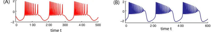
The types of the static bursting configurations in the Hindmarsh-Rose model shown in Figures1and2are also namedfold/homoclinicandfold/Hopf, as this would indicate that the terminal phases of the fast spiking and slow quiescent periods are de-termined, respectively, by a homoclinic bifurcation of a saddle equilibrium state, or a supercritical Andronov-Hopf bifurcation, along with a saddle-node bifurcation of equilibria, respectively, which all occur in the fast subsystem of the model. In the
Fig. 2 Top: a plateau-like or fold/Hopf bursting starts after the spiking manifoldMlcbecomes tangent to
the middle, saddle branch ofMeqand terminates further through the reverse supercritical Andronov-Hopf bifurcation on the upper depolarized branch ofMeq. Bottom: the primary feature of the square-wave bursting activity in the HR model also referred to as of fold/homoclinic type is the termination of the spiking manifoldMlc by the homoclinic bifurcation in the phase space of the fast subsystem. In both
cases: fold stands for a saddle-node bifurcation at the turning point (SN) on the lower, hyperpolarized branch ofMeq.
next section we will examine the transition bifurcation patterns between these types of bursting.
These manifolds, especially their stable branches, can be easily traced and visual-ized in the phase space by utilizing the slow variable as a sweeping parameter in the decoupled fast subsystem. Far from bifurcations, this slow-fast dissection approach allows for exhaustive simplifications that let one treat the dynamics of the full model as on overlay the uncorrelated dynamics of its fast subsystem mediated by repetitive passages of the slow variable.
onlyoccur in the full system. For example, this occurs when the dynamics of the fast subsystem falls to the time scale of the slow subsystem, particularly near saddle-node and homoclinic bifurcations. A classic example is the onset of chaotic dynamics of finite subshift shown by D. Terman [12] at the transition between tonic spiking and bursting that happens to be generic for a square-wave burster like the Hindmarsh-Rose model [13–15]. In addition [12] gives an explanation of common spike adding cascade in classical square-wave bursters which is due to a slow passage of the phase point near the saddle in the fast subsystem. Note that the nature of spike adding cas-cade could be bifurcationally different, as for example in the leech interneuron model due to the blue sky catastrophe [16] prolonging the burst duration phase, or because of homoclinics of a saddle periodic orbit [17,18] playing the role of the chaotic po-tential barrier, loosely speaking, that bursting should overcome to get an extra spike. Complex dynamics, including quick period doubling cascades in square wave bursters [19,20] can also be explained in terms of codimension-two homoclinic bifur-cations, including inclination-switch and orbit-flips, that occur at the transition [21,
22] from tonic spiking to bursting. Recent breakthrough examples of novel transitions to and from bursting due to reciprocal interactions of slow-fast dynamics include var-ious homoclinic of saddles and saddle-foci, the blue sky catastrophe, bistability due non-transverse homoclinics to saddle-node periodic orbits, canard-tori [13,16–18,
23–26]. The range of bifurcations and dynamical phenomena giving rise to bursting transcendsthe existing static classification schemes based solely on slow-fast dissec-tion.
In-depth understanding of the generic mechanisms combined into a broad global picture on the transition patterns between the activity types in typical models of indi-vidual neurons presents a fundamental challenge for the theory of applied dynamical systems. In response to variations of intrinsic parameters, or an external applied cur-rent, likeI in (1), a neuron model should demonstrate, migrate, and switch flexibly between various types of activities such as quiescence, tonic spiking and bursting. In addition, nonlinearity of the model can often imply bi- or multi-stability of several co-existing activities at the same parameter values. Bistability of coco-existing oscillatory patterns originate near global bifurcations taking place in the model. Multistability is well noticeable when a targeted activity can be robustly selected by choosing other initial conditions or by temporal perturbations, like applied external current. Having ascertained such a global picture we can make consistent predictions for determining basic principles of the functioning of coupled neurons on networks where they receive mixed, inhibitory and excitatory perturbations from other neurons and synergetically reciprocate.
structure oflimitsolutions of the system. Nevertheless, if performed extensively the brute force approach reveals adequately the backbone of the bifurcation structure of the model, which can be further enhanced and complemented with detailed bifur-cation analysis that would provide the finishing touches, in the form of bifurbifur-cations curves, to the initial brute force diagram. We point out that transformations reshaping bursting waveforms en route toward the tonic spiking activity are caused by atypical bifurcations due to the presence of two, or more time scales in bursting. Because of that bifurcations of stiff bursting solutions, especially irregular ones, are hard to trace down by parameter continuation software packages such as CONTENT and AUTO-based packages, which are specifically designed mainly for explorations of equilibria and ‘typical’ periodic orbits.
The primary goal of this paper is to demonstrate that straightforward methods used in neuroscience experimental studies can be as effective as conventional tools, based on the bifurcation and Lyapunov exponent theory, employed in nonlinear dynamics studies. In this paper, we revisit and examine transformations of various oscillatory activity types in the phenomenological Hindmarsh-Rose model of bursting neurons, viewed, so to speak, through the prism of neuroscience plausible methods. Next we compare our findings with the results obtained using the evaluation of a maximal Lyapunov exponent that was presented in detail in [27,28] which we consider as an etalon. More specifically, as a part of the comparison test, we place next to each other the bifurcation diagrams found using calculus-based computational tools yield-ing the whole spectrum of the Lyapunov exponents for complete solutions of the model and those obtained through examinations of 1D voltage traces, which are typ-ically available in experimental studies. We then extract various qualitative temporal characteristic of neuronal activity from non-transient fragments of such traces, in-cluding the number of spikes per regular burst, deviations of the spike numbers in case of chaotic bursting, interspike intervals, burst duration and period, and the duty cycle which is the ‘spiking’ fraction of the bursting period. By varying two control parameters of the model, we basically perform bi-parametric sweeps of its dynamics that are aimed to detect in a very straightforward manner various global bifurcations including•transitions between quiescence, tonic spiking and bursting activities in-cluding ones through various homoclinic bifurcations;•identify regular and chaotic transformation of bursting, including a change of the bursting topology accompa-nying square wave to plateau-like transitioning, as well as forward and backward sequences of spike-addition and -deletion, and so forth.
2 Materials and methods
The phenomenological system of ODEs proposed by Hindmarsh and Rose [29,30] for modeling bursting and spiking oscillatory activities in isolated neurons is given by:
˙
x=y−ax3+bx2−z+I,
˙
y=c−dx2−y, (1)
˙
z=εs(x−x0)−z
here,x is treated as the membrane potential, while y andzdescribe some fast and slow gating variables for ionic currents, respectively. Slow ‘activation’ ofzis due to the small parameter 0< ε1. The parameters in (1) are typically set as followsa= 1,c=1,d=5,s=4,x0= −1.6 andε=0.01, so that regular bursting oscillations
in the model at an ‘applied current’I=4, which belongs to the square-wave type at b=2.7, and transforms to a plateau-like bursting atb=2.52, see Figure1. Along with ‘intrinsic,’b, and ‘external,’I, bifurcation parameters the dynamics of the model are sensitive to variations to other parameters:εbeing treated as a rate of activation for some current, andx0being viewed as a control parameter delaying and advancing
the activation of the slow current in the modeled neuron. In response to variations of intrinsic parameters, or an external applied current, likeI in (1), a neuron model should demonstrate, migrate, and switch flexibly between various types of activities such as quiescence, tonic spiking and bursting.
In this section we will brief the core of the numerical techniques employed in the analysis of the HR model. We will start with the specifics of the numerical integration of the differential equations of the model (1).
There are a plethora of high quality numerical integrators that have been cre-ated by numerical ODEs specialists. This study utilizes a recently developed free-ware library TIDES (Taylor Integrator for Differential EquationS) available at
http://gme.unizar.es/software/tides[31].TIDESis a highly adaptive software pack-age for numerical simulations of ODE systems. While the Taylor method is one of the oldest numerical methods for solving ordinary differential equations, it is scarcely used nowadays but its use is growing in the computational dynamics community. The formulation of the method is quite simple. First consider the initial value problem
˙
y=f(t,y). The value y(ti)of the solution at ti can be evaluated as yi of the nth degree Taylor series ofy(t )att=ti (fis to be a smooth or analytical function). So, denotinghi=ti−ti−1,
y(t0)=:y0,
y(ti)yi−1+f(ti−1,yi−1)hi+ 1 2!
df(ti−1,yi−1)
dt h
2
i + · · · + 1 n!
dnf(ti−1,yi−1) dtn h
n i
=:yi.
Therefore, the problem is reduced to the determination of the Taylor coefficients 1/(j+1)!djf/dtj. This can be done efficiently by using automatic differentiation techniques (see details in [32]).
At this tolerance level theTIDESsoftware is as fast and slightly more accurate [31] than the codeDOPRI853developed by Hairer and Wanner [34]. Note thatTIDESis a general purpose software, and so it can be apply to general ODE systems, and not only to the HR model. We note also that we have employed the Taylor series method for solving variational equations and computations of the Lyapunov exponent spec-trum, which are viewed as nonstandard options for the method [35]. As remarked, in the numerical simulations it is possible to use several good general ODE solvers, but the main advantage of the Taylor method in this kind of studies is that it pro-vides most of the requirements we need for the problem, accuracy when needed, easy events detection, direct dense output as a power series and easy implementation of variational equations.
As mentioned above, the continuous output generated by the integrator based on the Taylor series method is able to detect accurately and effectively various instan-taneous events such as whether the phase point hits a cross-section or reaches some critical value like voltage maximum/minimum, or the number of spikes per burst ap-proaches the sought value, which is the underlying idea for the spike-counting (SC) technique [27]. In combination, the methods allows us to classify the solutions of the HR model in neuroscience terms: no spike - quiescence (convergence to a stable equilibrium point); single tonic spike - a round periodic orbit (like one around the manifoldMlc); multiple spikes within a train - bursting orbit composed of alternating
tonic spike and pseudo-quiescent periods, as well as distinguishing chaotic behaviors characterized by wide variations of spike numbers in burst trains. Besides, the SC-technique allows for indirect evaluations of the duty-cycle [DC] of the orbit, which is a fraction of the burst period (that is, the ratio[Burst duration]/[Burst period]) of regular, periodic dynamics. Long bursting implies a duty-cycle close to one, meaning that the neuron is active most of the time; on the other hand if DC is close to zero the neuron generates rare spikes, mostly staying in the quasi-quiescent state. Finally, the continuous output of the Taylor series is also used in constructing bifurcation diagrams based on the variability of intervals between the spikes.
3 Screening the HR model in the(b, I )-plane
The HR model can exhibit a plethora of dynamical activities at different param-eter values. Consequently, obtaining a comprehensive understanding of the multi-parametric evolution of a system like the HR model is no easy task, and hence most of the parameters are fixed in the model. In this section, the free bifurcation param-eters to be varied arebandI; both are in charge of transformations for the intrinsic structure of the fast subsystem in the HR model. Next we perform the two-parameter sweep or screen of the model to collect vital data representing the time and parame-ter transformations of the single ‘voltage’x-variable of the neuronal model. Further data mining will be carried out to extract quantitative and qualitative information about the dynamical variability of the model, bifurcations of its solutions, and so on. In Figures3and4 we use a homogeneous grid comprised of 1,000×1,000 points within the given parameter range. In short, that means that this scan represents 106
simulations.
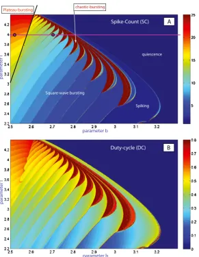
Figure3(A, B) presents the(b, I )-parameter spike-counting (SC) and duty-cycle (DC) diagrams of the HR model. Similar SC diagrams for the model were previously reported in [27]. The color-scale bar on the right in Inset (A) yields the number of spikes within a burst. The diagram for the duty-cycle evolution is shown in Inset (B). By combining these diagrams, we can partition the parameter plane into regions of different kinds of behaviors and classify the regimes: tonic-spiking (single spike), square-wave and plateau-like bursting, quiescence, and chaotic behaviors with the variability of spikes exceeding some preset limit. It is easy to see that both diagrams give consistent results. They reveal with clarity the region of tonic-spiking where both DC and SN take minimum values, below which there is the bursting region at the right bottom corner of the diagram. Bursting emerges from tonic spiking through the spike-addition cascade in two different ways: one is regular and reversible; the corresponding transitions are foliated by the bifurcation curves. The second kind of transitions is due to the clove-shaped regions (shown in red in Figure4) correspond-ing to well-developed chaotic dynamics in the model.
Another interesting behavioral phenomenon reshaping the type of bursting occurs in the top-left corner of the diagrams. In this region of bursting with a high num-ber of spikes transforms into bursting with a drastically lower numnum-ber of spikes per burst. To elucidate what happens on the border between these regions, we visually examined the orbits of the model. We found the border corresponding to the transi-tion between square-wave and plateau-like bursting (see the waveforms in Figure1
Fig. 3 (A)(b, I )-parameter sweep of the Hindmarsh-Rose model based on the spike-counting approach. The color-coded bar to the right gives the spike-number range. The diagram clearly shows the boundaries of the spike-addition sequence, and the border between square-wave and plateau-like bursting. It also reveals the clove-shape structure of the zones of chaotic bursting which adjoin to the regions of tonic-spiking. (B)Same-range screening based on the evaluation of the the duty-cycle of bursting. The duty cycle value comes close to one near the boundary between bursting and tonic-spiking and drops close to zero near the border of the spiking region. Compare (A) and (B) with the screening diagram based on the Lyapunov exponents for solutions of the model in Figure4below.
on the metamorphoses of the structure transformations. One can see that plateau-like bursting takes the place of square-wave bursting after the spiking manifold,Mlc,
be-comes tangent to the saddle branch of in the middle ofMeq and further terminates
on the upper depolarized branch ofMeqthrough the supercritical Andronov-Hopf
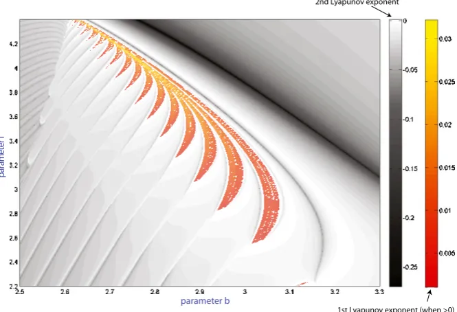
Fig. 4 Parametric sweeping of a Lyapunov exponent spectrum: orange-colored zones indicate chaotic dy-namics in the model, while a regular dydy-namics region is painted in grey colors of varying tint corresponding to a second Lyapunov exponent of zero value, and darker shades for negative values.
The HR model can exhibit complex, chaotic bursting with a large number of spikes, especially near transitions to hyperpolarized quiescence (see Figure3). In context of the dynamics of the model, bursting is technically treated as chaotic if trains have more than 25 unlike spikes with distinct interspike intervals. A large number of spikes can also be generated by periodic bursting. In order to differentiate between regular and chaotic bursting behaviors, we have also used another computa-tional technique. The complete spectrum of the Lyapunov exponents was evaluated for the orbits of the model as the two parameters were varied within the same range. In the simulations we discard a transient time of 103and we integrate till 105with the algorithm to compute the exponents and using as initial conditions the last value of the previous simulation. The corresponding sweeping diagram is shown in Fig-ure4. In the diagram, shown in the yellow-orange scale refers to the regions where the first Lyapunov exponent is positive. This means the occurrence of chaotic dy-namics in the model. The gray-colored regions are where the second Lyapunov ex-ponent is negative while the first Lyapunov exex-ponent remain zero on periodic orbits. The Lyapunov exponent based diagram also reveals the spike adding transitions, and the corresponding bifurcation lines can be drawn where the 2nd Lyapunov exponent reaches the maximal value of zero. This implies that the bifurcating bursting orbit is about to disappear and will be replaced by the successive bursting orbit with an ex-tra spike in each ex-train. Spike adding ex-transitions were observed and studied in several neuron models, including the Chay and Hindmarsh-Rose mathematical models [15,
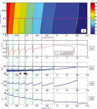
Fig. 5 (A)Magnification of the(b, I )-SC diagram in Figure3(A).(A1)First and second Lyapunov expo-nents plotted against the parameterb. Note that the second Lyapunov exponent of the bursting orbit raises to zero at the spike-adding transition and drops after.(A2)Interspike intervalvsbatI=2.4. Last inter-spike intervals in a burst increase at the inter-spike addition. This is an indication of the homoclinic bifurcation. (A3)Evolution of the duty-cycle and(A4)spike variability asbis varied.
scenarios for such cascades, including saddle-node bifurcations, homoclinic bifurca-tions of saddle equilibria [19,41] and periodic orbits [18], as well as through the blue sky catastrophe [21,22].
Fig. 6 Left: three-dimensional [3D] projections of three bursting orbits passing by the saddle. An extra spike is gained by the orbit after it has switched the outgoing directions determined by the unstable sepa-ratrices of the saddle.(A)-(D)Waveforms of four bursting orbits, shown in the phase space of the model on the left, at spike-adding or deletion bifurcations for the indicated parameter values ofIandb.
Indeed, the fact that the interspike interval grows by the end of the burst is a sig-nature of square-wave bursters. Recall that these bursters are also code-named fold/homoclinic meaning that the spiking, slow-motion manifold is terminated through a homoclinic bifurcation of the saddle that occurs in the fast subsystem of the model, see Figure2. The dwelling time of the phase point along the bursting orbit grows logarithmically fast the closer the point comes to the saddle [22]. The increase of the dwelling time is a generic phenomenon for all systems in a neighborhood of a saddle. What makes this phenomenon special for slow-fast systems is that the time scale of dynamics of the fast subsystem near the saddle turns out to be that of the slow subsystem, which gives rise to another peculiar phenomenon of ‘delayed loss of instability’ such that the phase point, previously turning around the spiking manifold, can be dragged along the middle, saddle branchMeqof equilibria possibly all the way
to the upper fold, provided that the timing is right, that is, the phase meets the saddle point right on the edge of the spiking manifold (lousily speaking, we encounter an-other kind of solutions broadly called ‘canards’, commonly characterized by the fact that a canard can follow an unstable branch of a slow-motion manifold). If the phase point reaches the edge before the saddle, it falls down to the hyperpolarized branch of Meqto start a new cycle of bursting. If the phase point travels past the saddle, then it
goes up along the other leading unstable separatrix of the saddle, makes another turn aroundMlc, resulting in the addition of an extra spike in the bursting orbit. Note that
when the phase point does not approach the saddle, the model generates bursts with same number of spikes. Again, let us emphasize that such a spike adding mechanism is typical for square-wave or fold/homoclinic bursters; however, underlying mecha-nisms for spike adding can be completely different even in square wave bursters, and other neuronal models [19,24,40,42], including the leech heart interneuron model [17,18].
4 Screening the HR-model in the(x0, I )and(x0, ε)-planes
In this section we examine the dynamics of the model in response to variations of the slow parameterε. In the neuroscience context,εcan be treated as the reciprocal ofτ, which determines the (in)activation rate of the slow current in a neuronal model. For the sake of consistency we will first screen the model in the(x0, I )-parameter plane,
while fixingb=3 andc= −3. Recall that the parameterx0moves the slow nullcline
of the model up and down in thex-direction (see Figure7). As the slow equation in (1) contains noy-variable, the plane in the (x, y, z)-phase space of the HR model, where the time derivativez˙vanishes, is the slow nullcline. One can see thatz <˙ 0 and
˙
z >0 below and above this nullcline, respectively. Note that a simple round periodic orbit on the tonic spiking manifold,Mlc, corresponds to regular tonic spiking activity
in the model. The position of the periodic orbit onMlcdepends on where the slow
nullclinez˙=0 cuts throughMlc. By changingx0, we make the periodic orbit shift
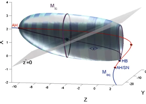
Fig. 7 (3D version of Figure2) Intersection point of the branchMeqwith the slow nullclinez˙=0 yields the equilibrium state of the HR model at givenx0. The dark blue point is the center of the gravity of the
stable periodic orbit of the HR model, which is depicted on the tonic spiking manifoldMlcatx0=1.8. It is located around the intersection point of the slow nullclinez˙=0 with the space curvexof the average
x-values on each periodic orbit that foliate the spiking manifoldMlc. The phase point, while turning aroundMlc, moves slowly toward the homoclinic edge (z >˙ 0) as long as it stays above the slow nullcline,
and goes backward (z <˙ 0) after it lowers below the slow nullclinez˙=0. When these opposite forces are canceled out over the revolution period, the phase point spins around the ‘center of the gravity’, that is, stays on the same periodic orbit. The variations ofx0move the slow nullcline and thus make the periodic orbit slide along the manifold. When the slow nullclinez˙=0 cuts through the unstable section ofMeq
between HB, standing for homoclinic bifurcation in the fast subsystem and the fold AH/SN, the model becomes a burster.
As it was said previously the HR model describes one of the most typical con-figurations of slow manifolds for square-wave bursting oscillations. First of all, the configuration needs the distinct Z-shape for the quiescent manifold,Meq, with the
lower branch corresponding to a hyperpolarized quiescent state of the neuron, while the upper unstable branch is surrounded by the spiking manifold,Mlc, foliated by
the stable limit cycles of the fast subsystem in the square bursting case. The branch regains stability in the case of plateau-like bursting. The manifoldMlc terminates
through the homoclinic bifurcation that occurs in the fast subsystem in the square bursting case. Between the lower fold and this homoclinic point, the system has a hysteresis which gives rise to bursting. In the bursting regime, the phase point of the HR model switches repeatedly between the spiking,Mlc, and quiescent,Meq,
mani-folds when it reaches their ends. In addition, both manimani-folds must be transient for the passing solutions of (1), that is,Meqmust be cut by the slow nullcline through the
middle, saddle branch belowMlcand above the hyperpolarized fold point. This
guar-antees thatMlcis also transient for the trajectories of the model that coil aroundMlc
while translating slowly towards the edge, which corresponds to the aforementioned homoclinic bifurcation. Thus, the rapid jump from the lower point onMeqtowards Mlc indicates the beginning of the spiking period of a burst followed by the resting
phase when the phase point drifts slowly alongMeqtowards the fold, onto which it
the phase point around the spiking manifold,Mlc, gives the number of spikes within
a burst, see Figures2and6. Bursting in the model takes place as long as the slow nullcline hitsMeqbetween the points labeled HB, corresponding to the homoclinic
bifurcation, and AH/SN standing for the singular Andronov-Hopf bifurcation in the full system, see Figure7.
Thus, by varyingx0we can make the model generate trains of bursts with various
number of spikes. It is easy to see that the value of the small parameterεdetermines the slow passage along both manifolds. So, halvingε should make bursts twice as long at least, with a doubled number of spikes. Note, too, that the duration of the quiescent phase should increase proportionally. As for variations ofI are concerned, Imoves, geometrically, the manifold horizontally in the 3D phase space of the model, in particular due to linearity of the slow equation in both variables. We show that because of that bothI andx0act similarly on dynamics; of special interest here are
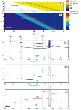
transitions between the activity type of the model, which this section is focused on. Figure8demonstrates the 2D(x0, I )-spike counting diagram withε=0.01 and
the same picture using the first and second Lyapunov exponents. The diagram re-veals a diagonal plot structure foliated by homogeneous bands. This suggests that variations of parametersI andx0cause similar responses in the model. On the band
structure there is a thin band of chaotic motion located inside the band of high num-ber of spikes, as remarked by the positive value of the maximum Lyapunov exponent. To gain insight into the band structure, we examine the evolutions of dynamics of the model as onlyx0 is varied at fixed current inputI =3.5. At smaller values of the
parameter, the model exhibits tonic spiking first, see Insets (C) and (E) of Figure8
presenting the interspike bifurcation diagram (IBC), and the spike counting (SC) di-agram. As the parameter is decreased further toward the bursting zone, the model enters a period-doubling cascade leading to chaos [20,43]. In Figure8(E) we see groups of spikes but without a clear bursting structure (bursting orbits withnspikes that doubles the period are denoted by 2×B(n)). Next, the model has a chaotic orbit (in region Ch), evolving into a compact chaotic region, which undergoes a bound-ary crisis, widening drastically the size of the chaotic attractor (also reported in [44,
45]). Asx0 is decreased further, chaos terminates through another boundary crisis
due to intermittency originating from a fold bifurcation. The model now generates regular trains of bursts. The corresponding bursting orbit further undergoes a series of period-doubling and period-halving bifurcations, before it steps into a cascade of spike deletion bifurcations, eventually leading to quiescence (Q) on the left hand side of of thex0-parametric pathway, after the Andronov-Hopf bifurcation.
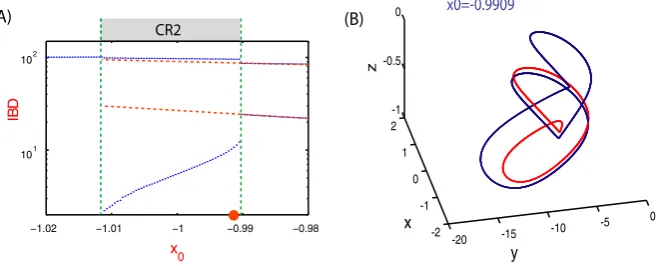
Figure9demonstrates the waveforms of the bursting solutions at selected points (shown in magenta) in Inset (C) of Figure8. One complete period of each waveform is squared out within a red box. Thus, we have the following orbits: a spiking orbit forx0= −1.12, two bistability points forx0= −1 and−0.9909, B(2)-orbit
(burst-ing with two spikes) forx0= −0.9, 2×B(3)-orbit forx0= −0.7, chaotic orbit for x0= −0.64 and again a regular spiking orbit atx0= −0.5 of a smaller period
com-pared to that atx0= −1.12. A quite interesting observation can be deduced from
Fig. 8 (A)2D(x0, I )Lyapunov exponents diagram atε=0.01;(B)2D(x0, I )spike-counting diagram
atε=0.01;(C)1D interspike-interval diagramvsx0forI=3.5;(D)Bursting duty-cycle dependence onx0;(E)Spike variability per burst is plotted againstx0.
is expanded in Figure10(A), and it reveals that there co-exist two distinct bursting orbits atx0=0.9909. The 3D phase projections and the corresponding waveforms,
Fig. 9 Tonic spiking and burstingx-traces at selected points on theb-parameter passway (shown in ma-genta) across the diagram in Figure8(C) showing several stages of spike addition transitions.
waveform. As was pointed out earlier such a coexistence of(n)-spike and(n+1) -spike bursts is a typical phenomenon for square-wave bursters at the -spike adding or deletion transitions due to ‘the delay loss of instability’ that occurs along the saddle, threshold branch ofMeqthat separates depolarized and hyper-polarized states of the
neuron model [41]. Recall that theoretically, due to the equal time scale dynamics of the fast subsystem near the saddle and the slow equation because of smallε, the phase point can be dragged along the saddle branch up to the upper fold onMeq.
Interestingly enough, the range of bistability zones will shrink as the value ofε is
increased. We would like to point out that multistability is a by-product of the nonlin-earity in the system. Multistability has been reported in several neuronal systems both experimentally and computationally, including individual neurons and their models, as well as in neural networks and multifunctional central pattern generators [1,46]. Multistability is of great interest for neuroscience as it can potentially enhance the flexibility of the nervous systems, decision making processes, and explain various nervous pathologies caused by sudden changes in system’s states.
Another peculiar observation related to the band structure in the(x0, I )-parametric
plane is concerned with the regions of high sensitivity to small variations of the con-trol parameterx0, whereas the overall band structure seems to be quite robust, or
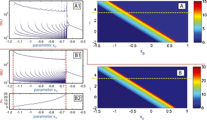
self-similar inI. This brings in one remaining question we would like to addresses in the paper: will this property of self-similarity of the band structure persist for smaller values ofε? Our findings are summarized in Figure11which demonstrates the bi-furcation diagrams for two values:ε=0.002 andε=0.001. They confirm that the band structure does persist and show predictably regions with larger number of spikes per bursts, especially forε=0.001 (compare the SC plot in 1D and 2D diagrams). To study the genesis of the band structure we also built the corresponding(x0, ε)
-diagrams shown in Figure12. Although both diagrams represent the same data of the spike-counting, the diagram on the right in Figure12is given in a logarithmic scale to demonstrate that the self-similarity property of the band structure is exponential inε. We can deduce from the diagrams that the most interesting, in terms of dynam-ics, region is contained between two curves (indicated by white dots). Within this region there are several diagonal bands corresponding to bursting orbits with differ-ent numbers of spikes. This plot explains the fact that a smallε-parametric cut will nevertheless reveal the band structure, observed in Figures8and11, thus confirming
Fig. 11 (A)2D spike-counting diagram projected to the plane(x0, I )atε=0.002;(A1)
interspike-dura-tion bifurcainterspike-dura-tion diagram forI=3.5.(B)2D spike-counting plot in the plane(x0, I )forε=0.001;(B1)
Fig. 12 (x0, ε)spike-counting diagram in the linear and logarithmic scales inε. Shown in blue and red
are regions of passive silence and intense spiking activities.
that either bifurcation parameterI orx0can be equality singled out to perform the
bifurcation analysis of the Hindmarsh-Rose model.
5 Conclusions
As of today, the Hindmarsh-Rose remains justifiably one of the most popular mathe-matical models, that describes, qualitatively well, the dynamics of a certain class of neuronal models derived using the Hodgkin-Huxley formalism. The model has been carefully analyzed using various mathematical and computational tools, and has been viewed though the prisms of the advanced bifurcation theory, geometric methods of slow-fast dynamical systems to reveal multiple peculiar qualitative features. Various brute force approaches [27,28] have been applied to the model to reveal its quantita-tive or metric properties though the examination of the Lyapunov exponent spectrum and the number of spikes per period.
myocytes - cardiac tissue cell. We showed in [26] that the proposed methods could provide the bifurcation details and add even problem-specific nuances into regulation control of temporal characteristics of realistic interneuron models of the leech. The evident advantage of the approach is its nativeness for the neuroscience community. Last but not least, it should emphasized that a 2D parameter sweeping of the model shown in Figures3and4takes about 10-20 times faster than the sweeping based on the Lyapunov exponents spectrum (Figure5). A drawback of the approach is that it needs to be corrected in cases where the model is multistable; this remains common weakness of all straightforward methods unless one uses randomized initial condi-tions and longer transients that could overall substantially prolong the simulation time.
It is in our future plans to broaden the applicability of these proposed computa-tional tools for studies of neuronal networks, especially for multifunccomputa-tional central pattern generators comprised of several neurons [2,46]. Such a multifunctional CPG is capable of generating multiple bursting rhythms at quite different time scale. It was shown recently in [3] that bursting outcomes of a multistable 3-cell network are determined by the duty cycle of bursting. Moreover, the longest bursting cell plays the role of the pacemaker of the network [47]. Note also that bursting network can be composed of individually tonic spiking cells that while inhibiting, even weekly, each other can create various bursting outcomes of the network as a whole. This indicates directly that such a cell, whether tonic spiking or bursting, is to be close to the bound-ary separating the activity types in the parameter space of distinct interneurons [25,
26], in particular to control effectively the temporal characteristic of bursting, regu-lar or chaotic. In the light of saying, it is evident that the tools native to neuroscience paradigms are suited more appropriately for studying bursting metamorphoses in net-works and the side-by-side comparison of the results of mathematical and experimen-tal studies using the common jargon. This computational toolkit shall bring us closer to the targeted goal - to build realistic and adequately responding models of concrete functional CPGs with specific time scales, phase locked states between synergetically coupled neurons with plausible bursting characteristics.
Competing interests
The authors declare that they have no competing interests.
Acknowledgements We would like to thank A. Neiman, J. Wojcik and B. Chung for very helpful com-ments. This work is supported by the Spanish Research project MTM2009-10767, and by NSF Grant DMS-1009591, RFFI Grant No. 08-01-00083, GSU Brain & Behaviors program, and MESRF ‘Attracting leading scientists to Russian universities’ project 14.740.11.0919.
References
1. Kristan, W.B.: Neuronal decision-making circuits. Curr. Biol.18(19), 928–932 (2008)
2. Shilnikov, A.L., Gordon, R., Belykh, I.: Polyrhythmic synchronization in bursting networking motifs. Chaos18(3), 037120 (2008)
4. Rinzel, J.: Bursting oscillations in an excitable membrane model. Lect. Notes Math.1151, 304–316 (1985)
5. Bertram, R., Butte, M.J., Kiemel, T., Sherman, A.: Topological and phenomenological classification of bursting oscillations. Bull. Math. Biol.57(3), 413–439 (1995)
6. Izhikevich, E.M.: Dynamical Systems in Neuroscience. The Geometry of Excitability and Bursting. MIT Press, Cambridge, MA (2007)
7. Tikhonov, A.N.: On the dependence of solutions of differential equations from a small parameter. Mat. Sb.22(64), 193–204 (1948)
8. Pontryagin, L.S., Rodygin, L.V.: Periodic solution of a system of ordinary differential equations with a small parameter in the terms containing derivatives. Sov. Math. Dokl.1, 611–619 (1960)
9. Fenichel, F.: Geometric singular perturbation theory for ordinary differential equations. J. Differ. Equ. 31, 53–98 (1979)
10. Mischenko, E.F., Rozov, N.K.: Differential Equations with Small Parameters and Relaxation Oscilla-tions. Plenum Press (1980)
11. Arnold, V.I., Afraimovich, V.S., Ilyashenko, Y.S., Shilnikov, L.P.: Bifurcation Theory, Dynamical Systems. Volume V. Encyclopaedia of Mathematical Sciences. Springer (1994)
12. Terman, D.: The transition from bursting to continuous spiking in excitable membrane models. J. Nonlinear Sci.2(2), 135–182 (1992)
13. Shilnikov, A.L., Calabrese, R., Cymbalyuk, G.: Mechanism of bistability: tonic spiking and bursting in a neuron model. Phys. Rev. E71(5), 056214 (2005)
14. Holden, A.V., Fan, Y.S.: From simple to simple bursting oscillatory behaviour via intermittent chaos in the Rose-Hindmarsh model for neuronal activity. Chaos Solitons Fractals2, 349–369 (1992) 15. Fan, Y.S., Holden, A.V.: Bifurcations, burstings, chaos and crises in the Rose-Hindmarsh model for
neuronal activity. Chaos Solitons Fractals3, 439–449 (1995)
16. Shilnikov, A.L., Cymbalyuk, G.: Transition between tonic spiking and bursting in a neuron model via the blue sky catastrophe. Phys. Rev. Lett.94(4), 048101 (2005)
17. Channell, P., Cymbalyuk, G., Shilnikov, A.L.: Origin of bursting through homoclinic spike adding in a neuron model. Phys. Rev. Lett.98(13), 134101 (2007)
18. Channell, P., Fuwape, I., Neiman, A.B., Shilnikov, A.L.: Variability of bursting patterns in a neuron model in the presence of noise. J. Comput. Neurosci.27(3), 527–542 (2009)
19. Innocenti, G., Genesio, R.: On the dynamics of chaotic spiking-bursting transition in the Hindmarsh-Rose neuron. Chaos19(2), 023124 (2009)
20. Wang, X.J.: Genesis of bursting oscillations in the Hindmarsh-Rose model and homoclinicity to a chaotic saddle. Physica D62(1-4), 263–274 (1993)
21. Shilnikov, A.L., Kolomiets, M.L.: Methods of the qualitative theory for the Hindmarsh-Rose model: a case study. A tutorial. Int. J. Bifurc. Chaos Appl. Sci. Eng.18(8), 2141–2168 (2008)
22. Shilnikov, L.P., Shilnikov, A.L., Turaev, D.V., Chua, L.O.: Methods of Qualitative Theory in Nonlin-ear Dynamics. Parts I and II. World Scientific Publishing Co. Inc. (1998) and (2001)
23. Feudel, U., Neiman, A., Pei, X., Wojtenek, W., Braun, H., Huber, M., Moss, F.: Homoclinic bifurca-tion in a Hodgkin-Huxley model of thermally sensitive neurons. Chaos10(1), 231–239 (2000) 24. Kramer, M.A., Traub, R.D., Kopell, N.J.: New dynamics in cerebellar purkinje cells: torus canards.
Phys. Rev. Lett.101(6), 068103 (2008)
25. Wojcik, J., Shilnikov, A.L.: Voltage interval mappings for dynamics transitions in elliptic bursters. Physica D240, 1164–1180 (2011)
26. Shilnikov, A.L.: Complete dynamical analysis of an interneuron model. Nonlinear Dyn. (2011 in press). doi:10.1007/s11071-011-0046-y
27. Storace, M., Linaro, D., de Lange, E.: The Hindmarsh-Rose neuron model: bifurcation analysis and piecewise-linear approximations. Chaos18(3), 033128 (2008)
28. de Lange, E., Hasler, M.: Predicting single spikes and spike patterns with the Hindmarsh-Rose model. Biol. Cybern.99(4-5), 349–360 (2008)
29. Hindmarsh, J.L., Cornelius, P.: The development of the Hindmarsh-Rose model for bursting. In: Burst-ing, pp. 3–18. World Sci. Publ., Hackensack, NJ (2005)
30. Hindmarsh, J.L., Rose, R.M.: A model of the nerve impulse using three coupled first-order differential equations. Proc. R. Soc. Lond. B, Biol. Sci.221, 87–102 (1984)
31. Abad, R., Barrio, R., Blesa, F., Rodríguez, M.: TIDES: a Taylor series Integrator for Differential EquationS. ACM T. Math Software, (2011 in press).http://gme.unizar.es/software/tides
33. Barrio, R., Blesa, F., Lara, M.: VSVO formulation of the Taylor method for the numerical solution of ODEs. Comput. Math. Appl.50(1-2), 93–111 (2005)
34. Hairer, E., Nørsett, S.P., Wanner, G.: Solving Ordinary Differential Equations. I, 2nd edn. Springer Series in Computational Mathematics, vol. 8, Springer-Verlag, Berlin (1993)
35. Barrio, R., Rodríguez, M., Abad, A., Blesa, F.: Breaking the limits: the Taylor series method. Appl. Math. Comput.167(20), 7940–7954 (2011)
36. Benettin, G., Galgani, L., Giorgilli, A., Strelcyn, J.M.: Lyapunov characteristic exponents for smooth dynamical systems and for Hamiltonian systems; a method for computing all of them. Part 2: Numer-ical application. Meccanica15, 21–30 (1980)
37. Wolf, A., Swift, J.B., Swinney, H.L., Vastano, J.A.: Determining Lyapunov exponents from a time series. Physica D16(3), 285–317 (1985)
38. Skokos, C.: The Lyapunov characteristic exponents and their computation. Lect. Notes Phys.790, 63–135 (2010)
39. Chay, T.R.: Chaos in a three-variable model of an excitable cell. Physica D16(2), 233–242 (1985) 40. Yang, Z., Qishao, L., Li, L.: The genesis of period-adding bursting without bursting-chaos in the Chay
model. Chaos Solitons Fractals27(3), 689–697 (2006)
41. Mozekilde, E., Lading, B., Yanchuk, S., Maistrenko, Y.: Bifurcation structure of a model of bursting pancreatic cells. Biosystems63, 2–13 (2001)
42. Innocenti, G., Morelli, A., Genesio, R., Torcini, A.: Dynamical phases of the Hindmarsh-Rose neu-ronal model: studies of the transition from bursting to spiking chaos. Chaos17(4), 043128 (2007) 43. Cymbalyuk, G., Shilnikov, A.L.: Coexistence of tonic spiking oscillations in a leech neuron model. J.
Comput. Neurosci.18(3), 255–263 (2005)
44. González-Miranda, J.M.: Observation of a continuous interior crisis in the Hindmarsh-Rose neuron model. Chaos13(3), 845–852 (2003)
45. González-Miranda, J.M.: Complex bifurcation structures in the Hindmarsh-Rose neuron model. Int. J. Bifurc. Chaos Appl. Sci. Eng.17(9), 3071–3083 (2007)
46. Briggman, K.L., Kristan, W.B.: Multifunctional pattern-generating circuits. Annu. Rev. Neurosci.31, 271–294 (2008)

![Fig. 6 Left: three-dimensional [3D] projections of three bursting orbits passing by the saddle](https://thumb-us.123doks.com/thumbv2/123dok_us/917933.1589701/12.439.55.388.53.217/fig-left-dimensional-projections-bursting-orbits-passing-saddle.webp)