Forestry & Natural-Resource Sciences Last Correction: Mar. 7, 2012
APPLICATION OF NUMERICAL METHODS FOR
CRASHWORTHINESS INVESTIGATION OF A LARGE
AIRCRAFT WING IMPACT WITH A TREE
Chao Zhang
1, Wieslaw K. Binienda
1, Frank E. Horvat
2, Wenzhi Wang
31
Department of Civil Engineering, University of Akron, 302 Buchtel Common, Akron, OH, 44325, USA
2
Department of Mechanical Engineering, University of Akron, 302 Buchtel Common, Akron, OH, 44325, USA
3School of Aeronautics, Northwestern Polytechnical University, Xian, Shaanxi 710072, China
Abstract.This paper demonstrates the application of a numerical methodology for a full-scale aircraft impact crashworthiness investigation. We studied the impact of an aircraft wing with a tree using LS-DYNA and ANSYS CFX. In particular, a detailed finite element model of the wing structure was represented as a box structure containing skin, spars and ribs, and fuel was represented as a distributed mass. We utilized several material models and verified them using leading-edge bird strike and wood bending experiments. Wood model Mat 143 with material parameters developed based on the wood bending test was found to be the most accurate in comparison with the experiment. We used the commercially available Computational Fluid Dynamics (CFD) software of ANSYS CFX to calculate the aerodynamic pressure distribution on the overall surface of the wing. The algorithm utilized the full three-dimensional Navier-Stokes equations for steady-state compressible fluid. LS-DYNA finite element model included aerodynamic pressures on the wings surfaces. Parametric studies showed that the tree model cannot destroy the lifting surface of the wing except the fragment of the leading edge. In every simulation scenario, the first spar of the wing cut through the tree and the upper part of the tree fell in the direction of the movement of the airplane.
Keywords: Full scale modeling, Finite Element Method, crashworthiness, nonlinear wood model, Mat 143, Johnson-Cook material model, fluid dynamics, aircraft, wing, tree.
1
Introduction
For aircraft crashworthiness analysis, it is important to consider the dynamic behavior of the aircraft un-der impact conditions. Because impact-related exper-iments are very difficult to conduct and very expen-sive, it is of great importance to develop alternative techniques to the experiments, such as analytical and computational methods to obtain an accurate simula-tion of aircraft structure response to any impact con-ditions. The finite element explicit codes, such as LS-DYNA, MSC.DYTRAN and PAM-CRASH, are widely used to simulate nonlinear, transient, dynamic events.
There were several studies published on the aftermath of the airplane crashes into the World Trade Center on September 11, 2001. These studies focused on the alu-minum wing cutting through the external steel columns of the building, the destruction of the airplane by the building core structure, and the reasons behind the col-lapse of the skyscrapers. Wierzbicki and Xue [21, 22, 23]
developed analytical and finite element models to study the resistance of the exterior columns, floors and core columns of the building to the impact of the airplane. It was found that the wing of the airplane would easily cut through the outer columns of the building with a cruis-ing speed of 240 m/s. The majority of the kinetic energy (about 50%) was dissipated by the floor, and the remain-ing plane energy dissipated at the buildremain-ing core columns. Bazant and Zhou [4] estimated that the temperatures in some sections of the building were elevated to 800˚C and 1000˚C due to a fire caused by burning jet fuel. Authors showed that these high temperatures induced the degradation or loss of the load-carrying capability of the steel structure in the floors, which were no longer able to support the weight of the building. Abboud [1] did a simulation study of the whole process – from im-pact, through the fuel spill and fire, to the collapse of the building using SAP2000 and dynamic nonlinear FLEX. The analysis demonstrated that while the robustness of the tubular-perimeter wall system and the redundancy
of the structure allowed the tower to resist immediate impact damage, the thermal loads overwhelmed the re-maining structural system capacity.
On April 10, 2010, a Polish Air Force Tupolev Tu-154M (registration number 101) performing a state flight from Warsaw (Poland) to Smolensk (Russia) crashed into the ground about 500 m short of the runway at Smolensk North Airport (XUBS). [11] reported that the aircraft’s left wing was brake off after collision with a birch tree before the crash. However, the role of a tree in breaking the wing is questionable. An analysis of air-craft impact with a tree has only rarely been published. Bocchieri [5] has recently presented a developed simula-tion of a full-scale experiment involving the crash of a Lockheed Constellation aircraft conducted for the US Department of Transportation. This experiment and simulation studied the process of aircraft wing impact into two telephone poles. The authors of this study used LS-DYNA with Mat143 to simulate the wood material of the poles. All simulations and high-speed video footage of the experiment revealed that the front spar of the wing cut through the telephone poles.
Morka et al. [15] investigated a circular cross-section beam impact with a stationary wing at a velocity of 10 m/s. In their model, the authors used LS-DYNA wood model *MAT 161/162 and *MAT 22, and they assumed relatively higher values of Young’s modulus and specific mass density for the aluminum alloy. They found that the effective plastic strain affects significantly the impact force of the wing on a stiff beam.
In the case of an airplane crash, the accurate impact process is very difficult to study. Numerical studies can help to verify a hypothesis generated during the crash investigation based on black boxes and other available data. We describe in this article a numerical study of the impact of a large passenger airliner (a Tupolev Tu-154M) with a birch tree. Through the simulation of this crash, we evaluated the damage to the wing considering a broad spectrum of parameters such as thickness of the structural components, velocity vector components, and various airplane configurations.
We conducted a three-point bending test of the birch to characterize the birch-tree material model. We used an artificial bird impact test into the leading edge of the wing to validate the aluminum material model. We used ANSYS CFX to simulate aerodynamic pressures on the surface of the wing. Through the integration of those pressures P(x, y),the resulting overall loads present on the wing surfaces have been determined. We present in the subsequent sections the methodology and results of the simulations of the impact between an airplane wing and a birch tree using the above material models and loading conditions.
2
Computational Model and Method
2.1 Aircraft Structure and Mesh A detailed finite element (FE) model of a full-scale Tu-154M aircraft was developed on the basis of data available from public sources. Many simplifying assumptions were made to keep the geometry simple and conservative. For exam-ple, doublers, joints, landing gears and fasteners were ignored. The development of the aircraft model was performed using HyperMesh10.0. Approximately 75,000 shell elements for each airplane wing and 3,400 shell ele-ments for the fuselage were used to model the solid part of the airplane. Coarse mesh with 57,200 solid elements and fine mesh with 288,000 solid elements were used to model the cone shape of the birch trunk. Figure 1 shows the overall view and finite element mesh of the impact model. In this study, the coordinate Y is inverse to the gravity direction, Z is the horizontal direction pointing from the tail to the nose of the airplane, while X is a line that runs along the leading edge of the left wing. The birch tree is cone-shaped and has a diameter of 0.44 m [9] at the impact height.
48 m
16
m
(a)
Z Y
(b) Y
X
Z
Figure 1: Overall view (a) and wing view (b) of the FEM for aircraft hit the tree
(a)
(b)
Figure 2: Inner structure and mesh of the wing
the root of the wing may be several times thicker than those at the wing tip. For example, the thicknesses of the wing skin may vary from 1.6 mm to 5 mm on the whole wing surface [6]. However, the thicknesses of the spar, rib and skin are assumed to be constant along the wing length. For parametric study, the thickness of the spar is assumed to be between 5 mm and 20 mm, the skin thickness is assumed to be between 1 mm and 5 mm, while the thickness of the ribs is assumed to be 3 mm based on knowledge of the aircraft structure and considering that the stringers, joints and bolts have been ignored.
2.2 Material Models The whole plane structure was assumed to be a V95 aluminum wrought alloy modeled with shell elements. The birch was assumed to be an orthotropic material modeled with solid elements. Sec-tion type #16 (*Fully Integrated Shell Element) was selected for the shell section to avoid loss of energy caused by hourglass. Concentrated masses were placed uniformly inside the wings to represent 8,000 kg of fuel. The total weight of the model is 87,000 kg, matching the estimated weight of the aircraft. Two material formu-lations were chosen for the airplane: one is a piece-wise
plasticity isotropic material model(*MAT 24) with an ultimate failure strain of 14%, and the other is nonlinear rate-dependent Johnson Cook model (*MAT 15) [8]. The material parameters for the models are presented in Tables 1 and 2.
Table 1: Input of piece-wise plasticity aluminum alloy model
Young’s modulus (MPa)
Yield stress (MPa)
Tangential modulus (MPa)
Poisson’s ratio
Density (kg/m3)
74000 444 573.8 0.33 2850
Table 2: Input of Johnson-Cook aluminum alloy models
Young’s modulus (MPa)
Shear modu-lus (MPa)
Poisson’s ratio
Density (kg/m3)
68900 25910 0.33 2700
Yield stress (MPa)
Strain hard-ening modu-lus (MPa)
Strain hardening exponent
Strain rate coefficient
324 114 0.4 0.002
The stress strain curves for the two material models are illustrated in Figure 3. The Johnson-Cook model shows a lower strength value but a higher failure strain. The performance of these two different material models will be discussed further under impact simulation.
0 100 200 300 400 500 600
0 0.05 0.1 0.15 0.2
Piece-wise JC-0.01/s JC-1/s JC-10/s JC-500/s JC-1000/s JC-2000/s
S
tre
ss
(
M
P
a)
Strain
Figure 3: Differences of two material models for the alu-minum alloy
me-chanical properties in the directions of three mutually perpendicular axes: longitudinal, radial and tangential, as shown in Figure 4. The longitudinal direction, also known as the grain direction, is parallel to the fiber; the radial axis is normal to the growth ring; and the tangential axis is perpendicular to the grain but tan-gent to the growth rings. Considering the cone geome-try of the birch,*AOPT=4.0was used to describe the birch as an local orthotropic material in a cylindrical coordinate system. Solid section type #1 (*Constant Stress Solid Element) with hour glass control type #6 (*Belytschko-Bindeman Strain Co-rotational Stiffness Form) was used for the birch solid elements. Data from public sources [12] were used to set mechan-ical properties of the birch, as shown in Table 3. The density value is obtained from testing of the birch lum-ber. The failure of the birch is determined based on a simple criterion:
ε1>εmax (1)
where ε1 is the maximum effective strain and εmax is
the effective strain at failure. The card*Add Erosion was included to define the failure of the birch in which the failure effective strain has been chosen as 5%.
Longitudinal
Tangential Radial
Figure 4: Three principal axes of wood
The wood model *MAT 143 in LS-DYNA (hence-forth referred to as Mat143) was primarily developed to simulate the deformation and failure of wooden guardrail posts impacted by vehicles [16]. The failure criterion of this wood model uses modified Hashin criterion, which contains tension, compression and shear in parallel and perpendicular modes. The advantages of this model in-clude rate dependent strength and yielding with asso-ciated plastic flow. This transversely isotropic material model was characterized based on three-point bending test results, with the parameters shown in Table 4. The stress strain curves of these two material models are compared in Figure 5. In this figure, it can be seen that the two models show completely different behavior.
One is linear elastic and the other has a large range of nonlinear plasticity and strain rate dependence.
0 6 12 18 24 30 36
0 0.05 0.1 0.15 0.2
0.01/s 1/s 10/s 20/s 80/s 100/s Orthelastic
S
tre
ss
(
M
P
a)
Strain
Figure 5: Differences of two material models for the wood
2.3 Selection of Contact Type As the impact with the birch tree occurs at the left wing, the fuselage and the right wing were considered as rigid bodies to increase computational efficiency. Since the right wing and fuse-lage are far away from the impact location, this assump-tion will not affect the impact failure behavior of the left wing. In LS-DYNA, for a connection between rigid bodies and a deformable body, it is recommended to use *Constrained. So in this model *Constrained Ex-tra Nodes Setwas applied to connect the fuselage and the left wing, and *Constrained Rigid Bodies was used to connect the right wing with the fuselage. Also in the wing structure, the spar built in the form of an I-beam contained web and flange shell elements. Con-nections are needed to attach the spar flange to the skin. Thus,*Tied Surface to Surfacecontact was defined to connect the spar flange and the wing skin.
For the impact process, *Automatic Surface to Surface card was chosen. This contact is defined for the three wing components (skin, spars, and ribs) and the birch tree. As the surface of the birch is approxi-mately circular,SOFT=2(Pinball segment based con-tact) was implemented for more stable computations. To avoid any material penetration,*Automatic Surface to Surface(No soft) was also defined between the skin and spar elements.
3
Validation of Material Models
exper-Table 3: Material parameters for orthotropic elastic wood model
Young’s Modulus (MPa) Poisson’s Ratio Shear Modulus (MPa) Density (kg/m3)
EL ER ET νLT νRL νRT GT L GLR GRT
10300 803.4 515 0.451 0.043 0.697 700.4 762.2 175.1 700
Table 4: Material parameters for LS-DYNA Mat143 wood model Parallel
modu-lus (MPa)
Perpendicular modulus (MPa)
Parallel shear modulus (MPa)
Perpendicular modulus (MPa)
Parallel Pois-son’s ratio
Density (kg/m3)
11400 243 588 87 0.39 700
Parallel tension strength (MPa)
Parallel com-pression
strength (MPa)
Perpendicular tension strength (MPa)
Perpendicular compression strength (MPa)
Parallel shear strength (MPa)
Perpendicular shear strength (MPa)
35.9 3.59E+07 3.45 3.75 9.9 14
iment was conducted, producing the load and deflection curves. This curve was compared with the numerical bending simulation results, and it proved the applica-bility of the wood material models. In order to validate the piece-wise plasticity and Johnson-Cook model, it was necessary to evaluate the usability of this material model on the application of other aerospace impact problems, such as a bird strike conducted in the lab. The numerical results matched well with experimental results.
3.1 Leading-edge Bird Strike Analysis A bird strike is a significant threat to an aircraft, as a collision with a bird during flight may lead to serious structural damage. The leading edge of the wing is one forward fac-ing component that is frequently studied for bird strike crashworthiness. A series of leading edge bird strike ex-periments [24] were conducted at Northwestern Poly-technical University in China. Based on the experimen-tal results, a finite element model in LS-DYNA was built to simulate the impact process and failure behavior. The results were then compared with the experimental and original simulation results.
(a) (b)
Figure 6: Experimental (a) and numerical (b) results of the deformed shape after impact
In this experiment, the leading edge was tied to a fixed supporting construction. The leading edge consisted of
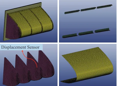
skin and 4 ribs. The gas gun was positioned in front of the sample with the muzzle pointing directly at the geo-metric center of the leading edge structure. The projec-tile was a 100 mm long gelatin cylinder with a diameter of 50 mm. The density of the gelatin was 1020 kg/m3. At a velocity of 153 m/s, the leading edge was not pen-etrated but developed a symmetric deformation area as shown in Figure 6 (a). The displacement of the mid-dle rib was recorded using a displacement sensor whose location is shown in Figure 7.
Displacement Sensor
Figure 7: Components and finite element mesh of the leading edge structure
5,022 Smooth Particle Hydro-dynamic (SPH) elements (projectile) and 7,648 solid elements (supporting frame). SPH is a powerful mesh free method and is considered to be the most efficient, experimentally validated for simu-lating a liquid-like material [10]. It was widely accepted to simulate the events related to bird strikes [13, 14].
Two kinds of contact definitions are used in the sim-ulation. One is *Automatic Nodes to Surface be-tween the projectile and the leading edge, the other one is *Tied Surface to Surface between each attached component of the leading edge structure. The piece-wise plasticity material mathematical representation was ap-plied to the leading edge structure. For the steel sup-porting construction, an elastic-plastic material model was assigned.
-1.6 -1.2 -0.8 -0.4 0 0.4
0.0007 0.0011 0.0015 0.0019
L
oa
d
(K
N
)
Time (s) Experiment Record Numerical Record
(a)
-6 -4 -2 0 2 4 6
0 2 4 6 8
D
is
p
la
ce
m
ent
(m
m
)
Time (ms) Experimental Record
Numerical Record
(b)
Figure 8: Experimental and numerical results of the load (a) and displacement (b) history
Figure 6 shows the experimental and simulation re-sults of the bird strike into the leading edge. The simu-lation contour captures the failure area fairly well. The plastic deformation expanded symmetrically and was
constrained in the horizontal direction by the ribs. The load history at the fix point and the displacement his-tory of the rib were also recorded and were compared with experimental data (as shown in Figure 8). The simulation results follow the experimental trend reason-ably well. However, the displacement history matches the first peak value perfectly.
3.2 Wood Bending Test and Modeling The wood three-point bending test was conducted to characterize the wood models. Using the ASTM standard D143 with some modifications based on the experimental condi-tions, the test was set up as shown in Figure 9 (a), with a loading span of 12 inches (304 mm). The dimension of the specimen was 25 by 25 by 410 mm with density of 698 kg/m3. The load was applied continuously throughout the test at a rate of motion of the moveable crosshead of 1.3 mm/min, and the force was recorded every second. In the simulation work, the bearing cylinders were mod-eled using *Rigid Wall in LS-DYNA. In Figure 9 (b), the white circles indicate the rigid walls in the simulation.
(a) (b)
Figure 9: Set up of three-point bending test: (a) exper-iment (b) simulation
The load was plotted against deflection curves as shown in Figure 10. The experimental and Mat143 curves show almost identical non-linear behavior while the orthotropic elastic model show linear behavior. The results indicate that the real wood may display some softening behavior during the loading process. Fracture energy of the wood described by the linear model (green line) is almost four times larger than the energy pro-duced in both the experiment (blue line) and Mat143 simulation (red line). A live birch tree is not dry; a liv-ing tree will be softer and weaker than the dry wood used in the three-point bending test. Hence, the simulation results produced using the selected dry-wood models are conservative. Morka et al. [15] also performed a three-point bending experiment, but their parameters for the birch tree are slightly different.
4
Evaluation of Aircraft Impact with
the Tree
0 2000 4000 6000 8000 10000
0 5 10 15 20
exp Mat143 Orth elastic
F
orc
e
(N
)
Displacement (mm)
Figure 10: Load vs. deflection curves of the modeling and experimental results
can be used to estimate the crash resistance between two colliding bodies. The structure with the higher solidity ratio is considered to cut through the one with the lower solidity ratio without being damaged. The solidity ratio, ρ, is defined as the ratio of structural massM divided by enclosed structural volumeV.
The structural volume is the volume enclosed by the outer periphery, not including the material volume. This value can be obtained from LS-DYNA model geometry. Taking an estimated mass Mwing=21500 kg and
vol-ume Vwing=23.65 m3, the solidity ratio of the wing is
ρwing =930 kg/m3. For the solid birch, the solidity
ra-tio is equivalent to its density, 700 kg/m3. According to the above factors, the wing should cut through the birch. During the impact of the wing into the birch, contact will mainly occur between the birch and the leading edge of the wing, or between the birch and the wing’s front spar.
Next, it is necessary to consider the impact resis-tance of the leading edge and the spar individually. For the leading edge only, the mass is much smaller, Mskin=2456.6 kg, while the enclosed volume is the same
as the wing structure,Vskin=23.65 m3. Its solidity ratio
is ρwing =104 kg/m3, which is much smaller than the
density of the birch. Thus the birch should damage the leading edge easily.
Using the same logic, the solidity ratio of the alu-minum alloy spar isρspar=2,700 kg/m3, a much higher
density than that of the birch (700 kg/m3). Hence, the front spar should cut the birch without any difficulty. It should be noted that the solidity ratio theory can only be used as an estimation because the dynamics of the impact are not taken under consideration. An accurate determination of the strength of the wing relative to the
strength of the birch requires a detailed dynamic finite element analysis.
4.2 Results of Finite Element Analysis In finite element analysis, simulations of a wing structure hitting a birch tree are performed. The initial conditions for the airplane impact are set within the following ranges: a flight velocity from 77.7 m/s to 80 m/s in the hor-izontal direction (vz) and from 0 m/s to 19.2 m/s in
the vertical direction (vy), a roll angle from 0˚ to 5˚
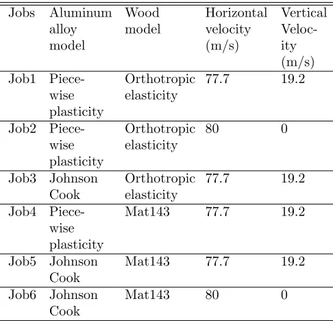
(left wing down), a pitch angle from 0˚ to 14˚ (upward from horizontal), and a yaw angle that is assumed to be 0˚. The flight velocity was assigned to the whole aircraft nodes using *Initial Velocity. Impact simu-lations were performed in LS-DYNA using a computer with an eight-core processor. The simulation of the first 0.05 s of the time after impact took about 20 hours of computational time. To obtain a comprehensive picture of the resulting damage and a good understanding of the performance of different material models, several com-binations of material models and velocity vector angles were selected for the simulations (Table 5).
Table 5: Summary of analyzed cases
Jobs Aluminum alloy model
Wood model
Horizontal velocity (m/s)
Vertical Veloc-ity (m/s) Job1
Piece-wise plasticity
Orthotropic elasticity
77.7 19.2
Job2 Piece-wise plasticity
Orthotropic elasticity
80 0
Job3 Johnson Cook
Orthotropic elasticity
77.7 19.2
Job4 Piece-wise plasticity
Mat143 77.7 19.2
Job5 Johnson Cook
Mat143 77.7 19.2
Job6 Johnson Cook
Mat143 80 0
to 0.022 s), the solid elements of the birch failed gradu-ally while no failure was observed for the spar elements. Reviewing the plastic strain history, it was found that most of the spar elements were in elastic range while the maximum plastic strain was only 0.025. These results agree with the preliminary predictions. The leading edge skin displayed little impact resistance while the spar is very strong and survives the impact load.
In summary, for every investigated vector velocity, for every used mesh, for every combination of considered material models, and for every configuration of the air-plane, the left wing of the airplane cuts the birch tree into two parts. The upper part of the birch receives an impulse that forces the tree to fall in the direction opposite to the motion of the airplane.
3.21 3.215
3.22 3.225 3.23 3.235 3.24
0 0.02 0.04 0.06 0.08 0.1 Total energy
Kinetic Energy
Time (second) (a)
E
ne
rgy (
×
1
0
8J)
energy
74 76 78 80 82 84
0 0.02 0.04 0.06 0.08 0.1
wing velocity
Smoothed velocity
Time (second)
V
el
oc
it
y
(m
/s
)
(b) Wing velocity
Figure 11: Energy (a) and velocity (b) history during the whole impact process
The energy and velocity histories for the impact are plotted in Figure 11. The node at the tip of the left wing was selected to record the velocity history. The energy plot shows an obvious decrease in kinetic energy
(red dashed line) for the first 0.022 s, which indicates that elastic deformation of the wing structure occurred during impact. The small decrease in total energy (blue line) was caused by the dissipation of energy during the impact in the form of sliding energy. After the birch tree was cut off, no energy dissipation occurred. As shown by the energy plot, both the kinetic and total energies are proportional. The subsequent increase of the energies is generated due to the springback process of the deformed wing.
The energy and velocity plots also demonstrate the two-stage damage process. The kinetic energy plot shows a faster decreasing rate after 0.01 s compared with the first 0.01 s. This is more obvious from the velocity plot, which shows that initially the velocity decreases slightly from 79.35 to 79 m/s during the first 0.01 s, but a steep decrease (from 79 to 76 m/s) occurs during the next 0.012 s.
The velocity of the aircraft’s tail was monitored to identify the plane’s rotation during the impact. As shown by the blue line in Figure 12 below, the tail moved to the right after the impact, which indicates that the front part of the plane moved to the left, as expected. At the same time, the vertical velocity (indicated by a red dashed line in the same figure) shows a steady linear decrease during the 0.1 s after impact.
18.4 18.6 18.8 19 19.2 19.4
-0.06 -0.04 -0.02 0 0.02 0.04 0.06
0 0.02 0.04 0.06 0.08 0.1 x velocity y velocity
X
V
el
oc
it
y
(m
/s
)
Time (second)
Y
V
el
oc
it
y
(m
/s
)
Figure 12: X and Y velocity history of the aircraft tail
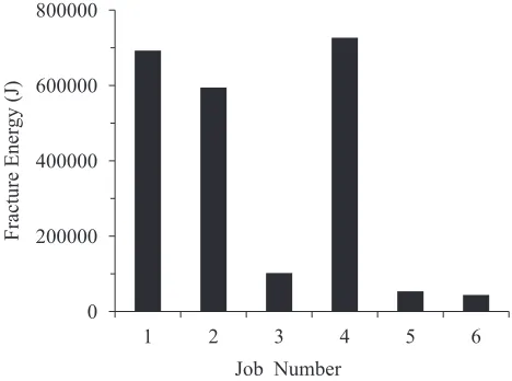
fracture energy was defined as the total internal energy of all the elements of the left wing.
0 200000 400000 600000 800000
1 2 3 4 5 6
Job Number
F
ra
ct
ure
E
ne
rgy
(J
)
Figure 13: Fracture energy of the wing for different nu-merical cases from Table 5
Using the selected six cases, it has been determined that the inclined cases with a vertical velocity of 19.2 m/s accumulated more fracture energy than the hori-zontal cases for the same airplane configuration with the pitch angle of 14˚. This difference may be due to the fact that a higher horizontal velocity will reduce the time of contact. The orthotropic elastic and Mat143 wood models display similar performance, while the Johnson-Cook model significantly lowered the fracture energy compared with the piece-wise plasticity model. How-ever, even with different material models and various impact angles, all the cases show nearly the same re-sults. The front spars in all cases cut the birch tree into two pieces. Since the case marked as Job4 in Table 5 pro-duces the highest fracture energy, additional parametric studies will be shown in the following section using Job4 material model, airplane configuration, velocity vector, and mesh.
Based on conducted parametric studies of all the cases from Table 5, it was concluded that the piece-wise plas-ticity aluminum-alloy model and the orthotropic elastic wood model (which were used in cases Job1 and Job2) provide the most conservative combination in the impact simulation.
4.3 Parametric Study of Material Thickness in the Wing Structure To further understand how the skin and spar thickness affected the degree of wing dam-age, we performed a parametric study of the thickness of the skin and the spars. The relationship of velocity reduction and eroding kinetic energy against the skin thickness (ranging from 1 mm to 5 mm) were plotted in
Figure 14. The velocity reduction is defined by differ-ence between the initial velocity and the velocity when the wing completely cuts off the birch tree. The eroding kinetic energy corresponds to the accumulative kinetic energy of the eroded skin elements. The velocity reduc-tions for all the thicknesses of the skin are very small, indicating that the skin has small resistance to the im-pact. With the increasing thickness of the skin, both the velocity reduction (green line) and the eroding ki-netic energy (blue line) displayed an increasing trend. The increased skin thickness slightly increases the re-sistance of the wing to impact. At the same time, the eroding kinetic energy increases proportionally to the in-crease of the skin mass. It was found that the variation of the skin thickness from 3 mm to 5 mm resulted in minimal variation in velocity reduction. Thus, increas-ing the thickness of the skin to 5 mm would not make a significant difference in resisting the impact.
0 0.3 0.6 0.9 1.2 1.5
48000 51000 54000 57000 60000 63000
1 2 3 4 5
Eroding Kinetic Energy Velocity Reduction
V
el
oc
it
y
Re
duc
ti
on
(m
/s
)
E
rodi
n
g
K
ine
tc
E
ne
rgy
(J
)
Thickness (mm)
Figure 14: Resultant velocity and eroding kinetic energy against skin thickness
Figure 15 displays the final plastic strain contour of the front spar for different thicknesses (ranging from 5 mm to 20 mm) at flight velocity vz=77.7 m/s and
vy=19.2 m/s. As the spar thickness decreases, the spar
(a) (b)
(c) (d)
(e) (f)
Figure 15: The final plastic strain contour of the spar with thickness of 20 mm (a), 17 mm (b), 13 mm (c), 10 mm (d), 8 mm (e) and 5 mm (f) at flight velocity vz=77.7 m/s andvy=19.2 m/s.
behind the front spar, it can be concluded that there is enough margin of safety for the wing to survive the im-pact with the birch tree under consideration for every studied spar thickness and impact scenario.
It is also observed that the top flange of the spar suf-fers more serious damage than the bottom flange. This is due to the positive vertical velocity of the plane, which caused compression contact between the birch tree and the top flange. The final plastic strain contours of a front spar with different thicknesses (ranging from 5 mm to 20 mm) at flight velocity vz=80 m/s are shown in Figure
16. Similar to the results shown in Figure 15, the spar el-ements suffer increasing plastic strain with the decrease of the spar thickness. In this case, the bottom flange suffers more damage because it touches the birch ear-lier. However, by comparing the damage for the same spar thicknesses in Figures 15 and 16, we can conclude that the case of a horizontal flying airplane produced less damage of the front spar than the cases with an inclined velocity vector (vz=77.7 m/s andvy=19.2 m/s).
5
Aerodynamic Pressures
During high speed flight, the pressure load produced by air flow is distributed over the airplane’s external sur-faces. For an accurate evaluation of the impact damage, the aerodynamic pressures need to be incorporated into the finite element model. In this section, the computa-tional fluid dynamic method (CFD) is used to calculate aerodynamic pressure profiles.
(a) (b)
(c) (d)
(e) (f)
Figure 16: The final plastic strain contour of the spar with thickness of 20 mm (a), 17 mm (b), 13 mm (c), 10 mm (d), 8 mm (e) and 5 mm (f) at flight velocityvz=80
m/s
5.1 CFD Modeling Methodology The air flow over the wing/plane profile yields a Reynolds number large enough that the resulting flow remains within the turbulent regime, meaning that the inertial forces are larger than the viscous forces. This dominance of iner-tial forces causes a degradation of the boundary layer due to the formation of eddies within the flow. To ac-count for this phenomenon, determine the transient fluc-tuations in the resulting velocity profile, and solve the unknown Reynolds stresses within the Reynolds Aver-aged Navier-Stokes equations (RANS), thek− model is used [18]. The Reynolds stress is a function of the tur-bulence kinetic energy (k) and the eddy viscosity (µt).
When the resulting Reynolds stress is substituted into the RANS, there are two resulting unknown terms: the effective viscosity (µef f) and the modified pressure (p0).
µef f =µ+µt (2)
p0 =p+2 3ρk+
2
3µef f∇ •U (3)
where ρ is fluid density and U, p and µ represent the instantaneous velocity vector, pressure and viscosity, re-spectively. The effective viscosity is a function of the eddy viscosity. In the k− model, the eddy viscosity is a function of the turbulence kinetic energy (k) and dissipation (),
µt=Cµρ
k2
(4)
where Cµ is a model constant. To determine the eddy
kandare determined.
∂(ρk)
∂t +∇ •(ρU k) =
∇ •
µ+µt
µk
∇k
+ Pk−ρ (5)
∂(ρ)
∂t +∇ •(ρU ) =
∇ •
µ+µt
µ
∇k
+
k(C1Pk−C2ρ) (6) whereµk,µ,C1 andC2 are all taken to be constants and Pk is defined as the turbulence production due to
viscous forces. The typical method for pressure calcu-lation utilizes a staggered grid approach to mitigate the “checker-board” type problems associated with the dis-cretization of the pressure derivative in the momentum equations over a control volume, as discussed in [3].
5.2 CFD Model Description Numerical results are obtained using ANSYS CFX, a commercial computa-tional engine used for multi-physics computacomputa-tional anal-ysis. The program has a powerful preprocessor, ICEM, which allows the input of complicated geometries as well as a post processor CFX-Post through which results can be presented in two- or three-dimensional format. The CFX algorithm is employed to solve the full, compress-ible Navier-Stokes equations in a Cartesian system of coordinates, using body-fitted coordinates. The solu-tion domain is divided into many cells called control volumes. Using a finite volume approach, the differ-ential equations are turned into a system of algebraic equations. They are numerically integrated over each of the computational cells, using a collocated cell-centered variable arrangement, where all dependent variables and material properties at the cell’s center are stored. For the momentum equations, a high resolution scheme is used that utilizes a combination of a first- and second-order upwind scheme. For pressure calculations, AN-SYS uses a pressure-velocity coupling that allows the Navier-Stokes equations to be solved in a coupled man-ner. This procedure is similar to the SIMPLEC scheme used in CFD-ACE+ and Fluent, which was originally proposed by both Van Doormal and Raithby [19] and later enhanced by Patankar and Spalding [17]. For SIM-PLEC, the equation for pressure correction is obtained from the continuity equation, and the scheme of veloc-ity and pressure calculations is fundamentally iterative in nature.
The fluid used throughout the numerical endeavor uti-lized air as an ideal gas for this steady, compressible, isothermal model. The resulting isothermal condition allows for calculation of the air density. Implementation
of the plane geometry and the subsequent wing profiles into the ANSYS pre-processor required boundary con-ditions similar to those shown in Figure 17. The figure illustrates how the fluid domain was defined with respect to the plane/wing geometry. The front and bottom of the rectangular domain were prescribed as inlet bound-ary conditions that allow for x and y components of velocity to be prescribed. Figure 17 shows the resulting components of the velocity vector, which yield an attack angle assumed to be between 0˚ and 20˚ with respect to the horizontal position of the wing. The top and end of the fluid domain were set to an outlet boundary con-dition. The outlet was prescribed with the same mass flow as that of the inlet condition. In addition, since this numerical work is to simulate a plane or portion of a plane in flight, the side walls of the domain were set to a no-shear boundary condition. The gridding of the domain utilized an unstructured mesh, where the density of elements near the wing/plane geometry in-creased. This increase in elements is required in order to accurately define the flow near and around the wing, in order to capture the development of the boundary layer and the eventual separation of the boundary layer as the angle of attack increases. The resulting unstruc-tured arrangement produced approximately 200,000 to 400,000 elements.
At 20 degree attack angle 77 m/s (in X)
19 m/s (in Y) No Shear Wall No Shear Wall
Outlet
Inlet
Figure 17: Overview of the boundary conditions used for the simulation of the wing/plane with the corresponding xandycomponent of velocity for an attack angle of 20˚
conver-gence criterion of 1.0 × 10⁻⁴ was used for each of the primitive variables (u,v,w, and p).
Upper Surface of Wing Lower Surface
of Wing Pressure
Contour
KPa
Figure 18: Super-imposed pressure contours on the lower and upper surface of the right wing profile for an attack angle of 20˚
(a) (b)
77 m/s
19 m/s
V Vortical cell
formation (a)
(b)
Figure 19: 2-D vectors and streamline velocity plots for an attack angle of 20˚ on two line sections of the wing: (a) close to the fuselage, (b) far from the fuselage.
5.3 CFD Simulation Results Figure 18 presents the results of the pressures generated on the lower and upper surfaces of the left wing for an attack angle of 20˚. It can be seen that the pressure distribution on the upper surface of the wing yields lower pressures, while larger pressures are generated on the lower surface of the wing. This difference in pressure is the lift force. The upper portion of the wing near the front edge yields even lower pressures than those on the rest of the wing. This lower pressure region is due to large velocity gradients being generated from the velocity of the air with respect to the front edge of the wing wall. These large velocities cause an overall decrease in pressure due to the Bernoulli Effect.
Figure 19 presents both two-dimensional superim-posed velocity vectors and velocity stream lines on two sections of the left wing surface for a 20˚ angle of at-tack. Figure 19(a) highlights the formation of the vor-tical cell displayed on a two-dimensional plane close to the fuselage. This vortical cell is produced as a result of large velocity and separation of the boundary layer. Consequently, the air can travel backwards or towards the front edge of the wing because of the boundary layer separation. Typically, the formation of such cells re-sults in lower pressure regions developing on the upper portion of the wing, as shown in Figure 18. Similar ve-locity profiles and vortical cell formations over another two-dimensional plane located far from the fuselage are shown in Figure 19(b).
(a) (b)
(c) (d)
(e) (f)
Figure 20: The final plastic strain contour of the spar with thickness of 20 mm (a), 17 mm (b), 13 mm (c), 10 mm (d), 8 mm (e) and 5 mm (f) included aerodynamic pressures loads.
struc-78.3 78.33 78.36 78.39 78.42
0 0.01 0.02 0.03
With aerodynamic pressure
No aerodynamic pressure
V
el
oc
it
y
(m
/s
)
Time (second) (a)
18.5 18.6 18.7 18.8 18.9 19
0 0.01 0.02 0.03
With aerodynamic pressure
No aerodynamic pressure
V
el
oc
it
y
(m
/s
)
Time (second) (b)
Figure 21: Comparison of resultant velocity (a) and vertical velocity (b) histories of the airplane with and without consideration of aerodynamic pressure
0 0.03 0.06 0.09 0.12 0.15
0 0.01 0.02 0.03
With aerodynamic pressure
No aerodynamic pressure
E
ffe
ct
ive
P
la
st
ic
S
tra
in
Time (second) (a)
0 0.03 0.06 0.09 0.12 0.15
0 0.01 0.02 0.03
With aerodynamic pressure
No aerodynamic pressure
E
ffe
ct
ive
P
la
st
ic
S
tra
in
Time (second) (b)
Figure 22: Effective plastic strain histories of spar (a) bottom flange elements and (b) top flange elements
ture and only slightly increased damage is observed in the front spar.
The velocity histories of the airplane with and without aerodynamic pressure are presented in Figure 21. The slightly higher vertical and resultant velocity matches with the aerodynamic effect when the airplane is flying upward, therefore proving the accuracy of the model.
For the I-beam structure, when impact occurs, the flanges are assumed to suffer normal stress while the web fails by shear stress. When the airplane flies up-ward, it has a vertical velocity, the top flange of the spar is compressed, and the bottom flange suffers mainly tension stresses. The effective plastic strain histories of the spar elements with a spar thickness 10 mm were also recorded, as shown in Figure 22. The top flange of the spar is damaged more seriously compared with the bottom flange. It is found that aerodynamic pres-sure causes higher effective plastic strain. For cases with
aerodynamic pressures (blue dashed line) and without aerodynamic pressure (red line), the plastic strains in-crease almost at the same time for the bottom and top flanges, as shown in both plots. Also, the effective plas-tic strains in both plots become constant at about 0.019 s after impact for both top and bottom elements. This result indicates that the aerodynamic pressure has no significant influence on the impact damage process.
6
Conclusions
1. An elastic-plastic dynamic finite element model for the impact of the aircraft wing with the birch tree was established. The numerical simulation was solved using nonlinear explicit FE code LSDYNA. The numerical results indicate that during impact, the leading edge of the wing is damaged over the length of 60–80 cm but the front spar cuts the birch into two pieces. The upper part of the birch should fall parallel to the direction of the airplane flight, which is consistent with the results of the experi-ment conducted with a Lockheed Constellation air-plane [5].
2. The leading edge bird strike simulations were con-ducted using the piece-wise aluminum alloy model, and the three-point bending of the birch tree was tested and compared with the wood models. All the material behavior simulations results are in good agreement with the experiments, indicating that the material models are well characterized.
3. Parametric studies were performed to (i) analyze how the thickness of the skin and the spar in the wing structure influences the degree of damage and (ii) investigate the critical thickness for the spar fail-ure. The results are shown qualitatively and quan-titatively. The spar thickness has been shown to be responsible for the crashworthiness of the wings.
4. Aerodynamic pressure profiles were calculated by ANSYS CFX, and the numerical results contained both velocity profiles and pressure contours over the wing/plane surfaces. The effects of aerodynamic pressure on impact behavior were investigated. It has been shown that the impact damage process is not significantly affected by the pressure loads, and plastic deformations are only slightly increased in some spar elements.
5. This study explored the potential ability of numer-ical simulation methods in crashworthiness studies of aircraft crash investigations. The FE simulation results successfully reproduced the aircraft impact scenario, and they may provide additional guide-lines and insights for aircraft design.
Acknowledgements
The authors would like to thank the four anonymous reviewers for their constructive suggestions and com-ments on the earlier version of this manuscript.
References
[1] Abboud, N., M. Levy, D. Tennant, J. Mould, H. Levine, S. King, C. Ekwueme, A. Jain, and G. Hart. 2003. Anatomy of a disaster: A structural investi-gation of the World Trade Center collapses. ASCE 3rd Forensic Congress, San Diego, California.
[2] Andryukhin, W.A., W.W. Efimov and N.B. Behtina. 2003. Construction and Strength of Airplanes. Ministry of Transportation of Russian Federation. Moscow State Techni-cal University of Civil Aviation. Moscow. http://storage.mstuca.ru/bitstream/123456789/ 1349/1/ .doc
[3] ANSYS, Inc. 2010. ANSYS CFX-Solver Theory Guide, Release 13.0 Canonsburg, Pennsylvania. http://www1.ansys.com/customer/content/docu-mentation/130/cfx thry.pdf
[4] Bazant, Z.P., and Y. Zhou. 2002. Why did the World Trade Center collapse? Simple analysis. Journal of Engineering Mechanical. 128(1): 2-6.
[5] Bocchieri R.T., R.M. MacNeill, C.N. Northrup, and D.S. Dierdorf. 2012. Crash simulation of transport aircraft for predicting fuel release: First phase-simulation of the Lockheed Constellation model L-1649 full-scale crash test. DOT/FAA/TC-12/43. US Department of Transportation, Federal Avi-ation AdministrAvi-ation, Atlantic City InternAvi-ational Airport, New Jersey.
[6] Boeing 737-800 structural repair manual.
[7] Buchar, J., S. Rolc, J. Lisy, and J. Schwengmeier. 2001. Model of the wood response to the high veloc-ity of loading. Proceedings of the 19th International Symposium of Ballistics, Interlaken, Switzerland. http://www.mif.pg.gda.pl/kft/Akron1/wood%20-model%20orthtropical%20elastic.pdf
[8] Buyuk, M., S. Kan, and M. Loikkanen. 2009. Ex-plicit finite-element analysis of 2012-T3/T351 alu-minum material under impact loading for airplane engine containment and fragment shielding. Journal of Aerospace Engineering 22(3): 287-295.
[10] Cleary, P.W., M. Prakash, J. Ha, and N. Stokes. 2007. Smooth particle hydrodynamics: Status and future potential. Progress in Computational Fluid Dynamics, an International Journal, 7(2): 70-90.
[11] Final report from the examination of the avia-tion accident no 192/2010/11 involving the Tu-154M airplane, tail number 101, which oc-curred on April 10, 2010 in the area of the SMOLENSK NORTH airfield. Committee for Investigation of National Aviation Acci-dents, Warsaw, Poland. http://mswia.datacenter-poland.pl/FinalReportTu-154M.pdf
[12] Forest Products Laboratory 2010.Wood Handbook,
Wood as an Engineering Material General Techni-cal Report FPL-GTR-190. United States Depart-ment of Agriculture Forest Service Madison, Wis-consin
[13] Lavoie, M.A., A. Gakwaya, and M.N. Ensan. 2008 Application of the SPH Method for Simulation of Aerospace Structures under Impact Loading. Pro-ceedings of the 10th International LSDYNA Users Conference, Dearborn, Michigan
[14] McCarthy, M.A., J.R. Xiao, C.T. McCarthy, A. Kamoulakos, J. Ramos, J.P. Gallard, and V. Melito. 2004. Modelling of bird strike on an aircraft wing leading edge made from fibre metal laminates – Part 2: Modelling of impact with SPH bird model. Ap-plied Composite Materials, 11(5): 317-340.
[15] Morka, A., T. Niezgoda, P. Dziewulski, and S. Stanislawek. 2012. Problems of numerical modeling of collision of bodies. Smolensk Conference, War-saw, Poland.
[16] Murray Y, J. Reid, R. Faller, B. Bielenberg and T. Paulsen. 2005. Evaluation of LS-DYNA wood ma-terial model 143. FHWA-HRT-04-096. US
Depart-ment of Transportation, Federal Highway Adminis-tration, McLean, Virginia
[17] Patankar, S.V., and D.B. Spalding. 1972. A cal-culation procedure of heat, mass and momentum transfer in three-dimensional parabolic flow. Inter-national Journal of Heat and Mass Transfer 15(10): 1787-1806.
[18] Patankar, S.V. 1980.Numerical Heat Transfer and Fluid Flow. McGraw-Hill. New York.
[19] Van Doormaal, J.P., and G.D. Raithby. 1984. En-hancement of the SIMPLE method for predicting incompressible fluid flows. Numerical Heat Trans-fer. 7(2): 147-163.
[20] Virtual aircraft design: Part 4 wing (In Russian) http://cnit.ssau.ru/virt lab/krilo/index.htm
[21] Wierzbicki, T., and X. Teng. 2003. How the air-plane wing cut through the exterior columns of the World Trade Center. International Journal of Im-pact Engineering. 28(6): 601–625.
[22] Wierzbicki, T., L. Xue, and M. Hendry-Brogan. 2002. Aircraft impact damage. In E. Kausel, (Ed.) The Towers Lost and Be-yond (pp. 31-64). Massachusetts Institute of Technology, Cambridge, Massachusetts. http://web.mit.edu/civenv/wtc/Towers%20Lost%-20&%20Beyond.pdf
[23] Xue, L., L. Zheng, and T. Wierzbicki. 2003. Inter-active failure in high velocity impact of two box beams. ASME 2003 International Mechanical Engi-neering Congress and Exposition, Washington, DC, USA.