http://theoryofcomputing.org
Proving Integrality Gaps without Knowing
the Linear Program
Sanjeev Arora
∗B´ela Bollob´as
†L´aszl´o Lov´asz
Iannis Tourlakis
Received: June 1, 2005; published: February 3, 2006.
Abstract: Proving integrality gaps for linear relaxations of NP optimization problems is a
difficult task and usually undertaken on a case-by-case basis. We initiate a more systematic approach. We prove an integrality gap of 2−o(1)for three families of linear relaxations forVERTEX COVER, and our methods seem relevant to other problems as well.
ACM Classification: G.1.6, F.1.3
AMS Classification: 68Q17, 90C05, 90C57
Key words and phrases: linear programming, inapproximability, approximation algorithms, NP-hard
problems, integrality gaps, lift-and-project, vertex cover
1
Introduction
Approximation algorithms for NP-hard problems—metricTSP, VERTEX COVER, graph expansion, cut problems, etc.—often use a linear relaxation of the problem (see Vazirani [31], Hochbaum [22]). For instance, a simple 2-approximation algorithm forVERTEX COVERsolves the following relaxation: min-imize ∑i∈Vxi such that xi+xj ≥1 for all {i,j} ∈E. One can show that in the optimum solution, xi∈ {0,1/2,1}. Thus rounding the 1/2’s up to 1 gives a VERTEX COVER [21]. This also proves an
upper bound of 2 on the integrality gap of the relaxation, which is the maximum over all graphs G of the ratio of the size of the minimumVERTEX COVERin G and the cost of the optimum fractional solution.
∗Supported by David and Lucile Packard Fellowship, NSF Grants CCR-009818 and CCR-0205594. Work done while
visiting Microsoft Research and the CS Dept at UC Berkeley.
†Research supported by NSF grant DSM 9971788 and DARPA grant F33615-01-C-1900
Can we write a linear relaxation with a lower integrality gap, say 1.5? Note that the LP need not even be of polynomial size so long as it comes with a polynomial time separation oracle, which is all we need to solve it with the Ellipsoid method.
Such quests for tighter relaxations can seem never-ending, since even simple modifications could conceivably tighten the relaxation. For certain problems, though, the quest for tighter relaxations— indeed, the quest for any better approximation algorithms—has ended. Results using probabilistically checkable proofs (PCPs) show that for a variety of problems such as MAX-3SAT, SET COVER, MAX -2SAT, etc., known approximation guarantees cannot be improved if P6=NP. Thus PCP-based techniques provide an explanation for our inability to provide tighter relaxations for these problems.
However, for many other problems, including all four problems mentioned in the opening paragraph, the PCP-based results are fairly weak or nonexistent and fall well below the integrality gaps of the best relaxations. The best hardness result forVERTEX COVER—due to Dinur and Safra [11], who improved upon a long line of work—only shows that 1.36-approximation is NP-hard. The best hardness result for metricTSPonly shows that 1.01-approximation is NP-hard [25], yet decades of work has failed to yield a relaxation with integrality gap better than 1.5 [32] (or 4/3, if one believes a well-known conjecture [17]). For graph expansion and related graph problems essentially no hardness results exist yet we only know relaxations with integrality gapΩ(log n)(Shmoys [29]).
When decades of work has failed to turn up tighter relaxations, one should seriously investigate the possibility that no tighter relaxations exist. However, proving such a statement may be related to P vs. NP, since linear programming is complete for P.1Thus it seems necessary to work with subfamilies of linear relaxations. An integrality gap result for a large subfamily of relaxations may then be viewed as a lower bound for a restricted computational model, analogous say to lower bounds for monotone circuits [27] and for proof systems [5]. An example is Yannakakis’s result [33] that representing TSP (the exact version) using a symmetric linear program requires exponentially many constraints—this ruled out some approaches to P=NP that were being tried at the time.
In this paper we prove nonexistence of tighter relaxations for VERTEX COVERamong three fairly general families of LPs. For all families we prove an integrality gap of 2−o(1). An interesting aspect of our result—also the reason for the paper’s title—is that no explicit description is known for the LPs in the three families. However, we can show that they use inequalities that have a fairly local view of the graph. This lets us construct graphs in which any minimum vertex cover must contain almost all the vertices (in particular, it must contain(1−α)n vertices whereα>0 is very small), yet the all-1/2 solution (or something close to it) is feasible for each inequality. Since the complement of a vertex cover is an independent set, and vice versa, our results may also be trivially rephrased to say that the integrality gap of the INDEPENDENT SET problem for our three families of LPs is unbounded, even though the graphs witnessing these gaps have independent sets of sizeΩ(n).
In the first two families of relaxations we allow only the variables x1,x2, . . . ,xn∈[0,1]for the vertices
and no auxiliary variables. Some such restriction seems necessary because auxiliary variables would give the LP the power of arbitrary polynomial-time computations. The third family allows auxiliary variables implicitly, but in a very controlled way—namely, as part of the “lift-and-project” procedure of
Lov´asz and Schrijver [24].
The first family consists of linear programs that can include arbitrary inequalities on any set ofεn variables, for some small constantε >0.
The second family consists of linear programs containing inequalities with low defect. Usually one defines “defect” for facets of theINDEPENDENT SETpolytope (see for instance [24,23]); here we will make an analogous definition for theVERTEX COVERpolytope (i.e., the convex hull of all integra vertex covers): The defect of aVERTEX COVERpolytope facet aTx≥b, where a is a vector of integers and b an integer, is defined to be 2b−∑iai. The defects of such facets are always non-negative [24]. Linear
programs in the second family are allowed those inequalities defining facets of the VERTEX COVER polytope with defect at mostεn. An integrality gap of 2−o(1)for this family is a simple corollary of the one for the first family.
The third family consists of linear programs obtained from O(log n)rounds of a “lift-and-project” construction of Lov´asz and Schrijver [24]. This is a method that underlies semidefinite relaxations used in many recent approximation algorithms starting with Goemans and Williamson [19]. The LS proce-dure over many rounds generates tighter and tighter linear relaxations for 0/1 optimization problems. It is more round-efficient than classical cutting planes procedures such as Gomory-Chv´atal [8] since it generates every valid inequality in at most n rounds. Even in one round it generates nontrivial inequali-ties forVERTEX COVER. Furthermore, the set of inequalities derivable in O(1)rounds—this could be an exponentially large set—has a polynomial-time separation oracle, thus allowing the Ellipsoid method to optimize over this set. In general, one can optimize over the set of inequalities obtained after r rounds in nO(r)time. We show that at leastΩ(log n)rounds of the LS procedure (the LP version, not the
semidef-inite version) are necessary to reduce the integrality gap below 2−o(1).2 Note that characterizing the set of inequalities obtained in even O(1)rounds has proved difficult; even the case of 2 rounds is open.
For the first family, better integrality gaps can be obtained forINDEPENDENT SETthan those triv-ially implied by our results forVERTEX COVER. We show that for linear programs where each inequality uses at most nε(1−γ)variables (here
ε,γ>0 are any small constants), the integrality gap forINDEPEN -DENT SETis n1−ε. This is essentially tight since constraints using nε variables can clearly approximate INDEPENDENT SETwithin a factor of n1−ε.
Our techniques seem applicable to problems other thanVERTEX COVER(andINDEPENDENT SET) and have been the subject of future work [6, 1,30]. These developments are discussed in the related work section below. However, several open problems remain. For example, extending our ideas to semidefinite relaxations as well as to the semidefinite programming analogue of the Lov´asz-Schrijver procedure remains a difficult and interesting open problem. We discuss this and other open problems further inSection 5.
We also note that the integrality gaps proven inSection 2are strong enough (namely, they apply to LPs that we do not know how to solve in 2o(n) time) that they may be seen as complementary to PCP-based results. Even if it were shown using PCPs that(2−ε)-approximation toVERTEX COVERis NP-hard, the proof would probably involve even more complex reductions than those in [11]. Thus it
might reduce 3SATformulae of size n toVERTEX COVERon graphs of size nc, where c is astronomical. Even if we assume 3SAThas no 2o(n)time algorithms, such a reduction would not rule out an integrality gap of 1.1 (say) for the relaxations in Section 2. In other words, even in a world with PCP-based results, our methods may be useful for ruling out subexponential approximation algorithms that use linear programming approaches.
Related work A few authors have viewed the Lov´asz-Schrijver procedure as a proof system and shown thatΩ(n)rounds are required to derive certain simple inequalities (e.g., Goemans and Tunc¸el [18], Cook and Dash [9]). However, these papers do not consider the issue of how the integrality gap improves (or fails to improve) after a few rounds of the LS procedure. A recent (and independent) paper by Feige and Krauthgamer [16] considers the question of integrality gaps, but for the maximumCLIQUEproblem on a random graph with edge probabilities 1/2. They show thatΩ(log n)rounds of LS+, the semi-definite
version of Lov´asz and Schrijver’s lift-and-project procedure, are necessary and sufficient to reduce the integrality gap to 1 (with high probability over the choice of the graph). However, this result does not directly give any lower bound on the approximability ofVERTEX COVER, since in their graphs both the minimum (integral) vertex cover and the optimal value of the relaxations considered are about n.
Subsequently to our work there have appeared several papers proving integrality gaps for relaxations using both the LP and SDP versions of the Lov´asz-Schrijver lift-and-project method. Buresh-Oppenheim et al. [6] show that Ω(n) rounds of LS+ are needed to obtain relaxations for MAX-kSAT, k≥5, with
integrality gaps less than(2k−1)/2k−ε. Alekhnovich et al. [1], building upon [6], show thatΩ(n) rounds of LS+are needed to obtain relaxations forMAX-3SATwith integrality gaps less than 7/8−ε. In addition they showed thatΩ(n)rounds of LS+are needed to obtain relaxations forSET-COVERand
rank-k hypergraphVERTEX COVERwith integrality gaps less than(1−ε)ln n and k−1−ε, respectively. Note that PCP-based results (such as those of H˚astad [20], Feige [15] and Dinur et al. [10]) already ruled out non-trivial polynomial-time approximation algorithms for these problems (assuming P6=NP). However, they did not rule out slightly subexponential approximation algorithms (defined as those running in 2nc time for c<1) for the reasons mentioned earlier, namely, the blowup in instance size caused by the PCP-based reductions.
Tourlakis [30], building on techniques used in the current paper, proved thatΩ(log log n)rounds of LS are needed to obtain relaxations for rank-k hypergraph VERTEX COVER with integrality gaps less than k−ε.
2
The first family
In this section we prove integrality gaps for linear programs in{x1,x2, . . . ,xn}for bothVERTEX COVER
The natural candidate graph for exhibiting integrality gaps for these relaxations would be one where the largest independent set has size at mostαn for some small α>0, but every induced subgraph on εn vertices has an independent set of size nearlyεn/2. However, it turns out that the local property we need for our graph is somewhat stronger: all small induced subgraphs have small fractional chromatic number which we define below.
We will construct the required graph by the probabilistic method inTheorem 2.3. This result appears to be new, although it fits in a line of results starting with Erd˝os [13] showing that the chromatic number of a graph cannot be deduced from “local considerations” (see also Alon and Spencer [2], p.130).
Definition 2.1. A fractionalγ-coloring of a graph G is a multisetC={U1, . . . ,UN}of independent sets
of vertices (for some N) such that every vertex is in at least N/γmembers ofC. The fractional chromatic
number of G is
χf(G) =inf{γ: G has a fractionalγ-coloring} .
Note that if G has a k-coloring with color classes U1, . . . ,UkthenC={U1, . . . ,Uk}is also a fractional k-coloring of G. Consequently,χf(G)≤χ(G).
Remark 2.2. Ifχf(G) =γ and{U1, . . . ,UN}is a fractionalγ-coloring for G, we will usually assume
without loss of generality that each vertex of G (by deleting it from a few of the Ui if necessary) is in exactly N/γsets.
Note that strictly speaking, having χf(G) =γ does not guarantee that there exists a fractional γ
-coloring for G; it only guarantees a fractional(γ+ε)-coloring for allε>0. Nevertheless, in the interest of keeping our notation clean, we will always assume that a fractionalγ-coloring does exist (in particular, we will only consider rationalγ). This slight inaccuracy will not affect the validity of our arguments.
Theorem 2.3. Let 0<α,δ <1/2 be constants. Then there exist constantsβ =β(α,δ)>0 and n0=
n0(α,β,δ)such that for every n≥n0there is a graph with n vertices and independence number at most
αn such that every subgraph induced by a subset of at mostβn vertices has fractional chromatic number
at most 2+δ.
Let H be the graph constructed inTheorem 2.3withα,δ arbitrarily close to 0 and letβ be as given by the theorem.
Theorem 2.4. The vector with all coordinates 1+δ
2+δ is feasible for any linear relaxation for H in which each constraint involves at mostβn variables. Consequently, since any independent set is the
comple-ment of a vertex cover, and vice versa, the integrality gap is at least(1−α)·21++δδ.
Proof. It suffices to show that the all-1+δ
2+δ vector is feasible for any set of constraints AI·x≤bI where I⊆ {1, . . . ,n}has size at mostβn.
So fix any subset I of at mostβn vertices and let{U1, . . . ,UN}be a fractional(2+δ)-coloring for I
such that each vertex in I is in exactly a 1/(2+δ)fraction of the Ui’s (seeRemark 2.2). Note that each I\Ui is a vertex cover in the subgraph induced by I and hence can be extended to a vertex cover of the
entire graph. By definition, the characteristic vector of any such vertex cover extension obeys AI·x≤bI.
So since these constraints only involve variables from I, it follows that any vector inRn that has 1I\Ui
Consider the vectors v1,v2, . . . ,vN∈Rnwhere viis equal to 1I\Ui in those coordinates corresponding
to I and is(1+δ)/(2+δ)otherwise. Each such vector satisfies AI·x≤bI, so convexity implies that
the same is also true for the average vectorN1(v1+v2+· · ·+vN). Since each vertex in I lies in exactly
a 1−1/(2+δ) = (1+δ)/(2+δ)fraction of the vertex covers, this average is the all-12++δδ vector. Thus this vector satisfies AI·x≤bI, as desired.
Note that the same construction can also be used to prove integrality gaps for linear relaxations for INDEPENDENT SET:
Corollary 2.5. EveryINDEPENDENT SETlinear relaxation for H (where H is the same graph as above) where each constraint in the relaxation has at mostβn variables has integrality gap at least α(21+δ).
Proof. Let I be any subset of at mostβn vertices and let{U1, . . . ,UN}be a fractional(2+δ)-coloring
for I such that each vertex in I is in exactly a 1/(2+δ)fraction of the Ui’s (seeRemark 2.2). Now define
vectors v1,v2, . . . ,vN ∈Rnas follows: Let vi equal 1Ui in those coordinates corresponding to I but have
viequal 1/(2+δ)outside I. Then each vi is feasible for all constraints involving variables only from I.
But then, the average of the vi’s, i.e., the vector with all coordinates 1/(2+δ), is also feasible for these
constraints.
Denote the size of the maximum independent set in a graph G byα(G). The above argument in fact yields the following more general theorem.
Theorem 2.6. Let G be a graph on n vertices such that every subgraph induced by a set of at mostβ(n)
vertices has fractional chromatic number≤C. Then the vector with all coordinatesC1 is feasible for any linear relaxation of theINDEPENDENT SETconstraints for G in which each relaxed constraint involves at mostβ(n)variables. Consequently, the integrality gap for the relaxation is at least α(Gn)C.
This suggests we can obtain larger integrality gaps for INDEPENDENT SET if we further limit the number of variables in each constraint. InSection 2.2below we show that this is indeed the case by exhibiting graphs for whichTheorem 2.6yields the following:
Theorem 2.7. Fixε,γ>0. Then there exists a constant n0=n0(ε,γ)such that for every n≥n0there
exists a graph G with n vertices for which the integrality gap of any linear relaxation forINDEPENDENT SETin which each constraint uses at most nε(1−γ)variables is at least n1−ε.
2.1 Proof ofTheorem 2.3
We then show in Lemma 2.13 that every high girth graph satisfying this sparsity condition has fractional chromatic number 2+δ on every induced subgraph with at mostβn vertices. The proof uses induction on the subgraph size. The main idea in the inductive step is to exhibit a long path inside every subgraph using Lemma 2.12. Peeling away the path gives a smaller subgraph that is colored (fractionally) using the inductive assumption.Lemma 2.11is then used to extend this fractional coloring, completing the induction.
Now we give details. The next lemma concerns the “standard random graph theory” mentioned above, together with the new sparsity condition.
Lemma 2.8. Given real numbersα,η with 0<α<1/250 and 0<η<1/2, letλ>e2andβ >0 be
such that
2logλ
λ ≤α (2.1)
and
β<(eλ)−2/η . (2.2)
Let g≥3 be an integer such that g≤log n/(3 logλ). Then there is an integer n0=n0(λ,η,g)such that
for every n≥n0 there is a graph H of order n, girth at least g and independence number at most αn
such that every subgraph of H with`≤βn vertices contains at most(1+η)`edges.
Remark 2.9. Condition (2.1) is satisfied if we take
λ = (3/α)log(1/α) .
Proof ofLemma 2.8. Let us consider the space of random graphsG(n,p)with p=λ/n. We will show that a graph Gn,pdrawn randomly from this space, modulo a few small alterations, satisfies with high
probability the three properties required of H in the statement of the lemma. Let 0<α0<α be such that
1+log(1/α0)<λ α0/2 . (2.3)
Inequality (2.1) implies that we can choose such anα0. In order to avoid unnecessary clutter, in what
follows, we shall drop the integrality signs (in particular, we shall writeα0n instead ofdα0ne); this slight
inaccuracy will not endanger the validity of the arguments. Also, as usual, we shall assume that n is large enough to make our inequalities hold.
1. The probability that for some`, 4≤`≤1/η, some`-set in Gn,p spans at least`+1 edges is at
most
1/η
∑
`=4
n `
`
2
`+1 λ
n `+1
≤ 1/η
∑
`=4
en
`
` e`(`+1)
2
`+1 !`+1
λ
n `+1
= 1
en
1/η
∑
`=4
`
e2λ 2
`+1
Similarly, the probability that for some`, 1/η< ` <βn, some`-set spans at least(1+η)`edges is at most
βn
∑
`=1/η
n ` ` 2
(1+η)` λ
n
(1+η)`
≤
βn
∑
`=1/η
" en
`
e`
2(1+η)
1+η λ
n
1+η#`
≤
βn
∑
`=1/η
e2(`/n)η
λ1+η` . (2.4)
We bound (2.4) by first splitting the sum into two quantities and bounding each of them: Letting C=e2λ1+η we have that,
√ n
∑
`=1/η
e2(`/n)η
λ1+η`≤
√ n
∑
`=1/η
C √ n ` = C √ n 1/η+1
1−(C/√n)
√ n−1/η
1−(C/√n) =O(n
−1) .
On the other hand, (2.2) implies that D=e2βηλ2<1, and hence,
βn
∑
`=√n+1
e2(`/n)η
λ1+η`≤
βn
∑
`=√n
D`≤D
√ n+1
1−D =O(n −1) .
So, (2.4) is at most O(n−1).
Hence, the probability that all `-sets, `≤βn, in Gn,p span at most (1+η)` edges is at least 1−O(n−1).
2. Let I=I(Gn,p)be the number of independent sets ofdα0nevertices in Gn,p. Note that
E(I) =
n
α0n
1−λ
n (α0n2 )
≤
e
α0
e−λ α0/2
α0n
=γ0α0n .
Inequality (2.3) implies thatγ0<1, so the probability that Gn,pcontains an independent set ofα0n
vertices is exponentially small.
3. Call a cycle in Gn,p short if its length is less than g. The expected number of short cycles is less
than
g−1
∑
`=3 n` ` λ n ` =g−1
∑
`=3
λ` ` ≤n
1/3 .
By Markov’s inequality, Gn,phas at most n1/2short cycles with probability at least 1−O(n−1/6).
Deleting an edge from each of these cycles then gives a graph of girth at least g.
Consequently, with probability 1−O(n−1/6), Gn,phas no set of`≤βn vertices spanning more than (1+η)`edges, and moreover, if we delete an edge from each short cycle then the independence number of the new graph H=G0n,pis at most
α0n+ √
n<αn .
Now we establish some basic properties ofχf. It is easy to check that a path with at least one edge
has fractional chromatic number 2. In particular, a graph has fractional chromatic number less than 2 if and only if it is an independent set. The proof of the next lemma is left to the reader.
Lemma 2.10. 1. If Ckdenotes the cycle of length k thenχf(C2`) =2 andχf(C2`+1) = (2`+1)/`.
2. If|V(G1)∩V(G2)| ≤1 thenχf(G1∪G2) =max
χf(G1),χf(G2) .
The next Lemma concerns the fractional chromatic number of a graph that contains a long path (i.e., the vertices on the path’s interior have no edges outside the path edges).
Lemma 2.11. Let`≥2 and let G be a graph obtained by adding a path x0x1. . .x`+1 to a graph G0,
where x0,x`+1∈V(G0)and xi6∈V(G0)for 1≤i≤`. Thenχf(G)≤max{χf(G0),`2−`1}.
Proof. Letχf(G0) =1/γ and suppose first thatγ>1/2. Then G is an independent set and the lemma follows since paths have fractional chromatic number 2.
So assumeγ ≤1/2. By Remark 2.2we can assume without loss of generality that there exists a multisetC0={U10, . . . ,UN0} of independent sets in G0 such that every vertex of G0 is in exactlyγN of these sets. So since x0∈G0andγ≤1/2, there exists a multisetAcontaining exactly N/2 sets fromC0
such that no set inAcontains x0. Similarly, there exists a multisetBof N/2 sets taken fromC0such that
no set inBcontains x`+1.
Fix i, 1≤i≤n. We will define a colouringCi for G\ {xi}(i.e., G with xi removed) by extending
the sets Uh0 inC0to independent sets Uhin G\ {xi}. Moreover, our colouring will have the property that
each xj, 1≤ j≤`, j6=i will be in exactly half the sets ofCi. Our approach will be as follows: Fix a set Uh0∈C0. If Uh0∈Awe will then add to Uhevery other node in the path fragment from x1to xi−1starting
with x1: That is, x1,x3,x5, . . .will be in Uh, but x2,x4, . . .will not. If instead Uh0 6∈Athen x2,x4,x6, . . .
will be in Uh, but x1,x3, . . .will not. Similarly, we will decide which of the nodes xi+1,xi+2, . . . ,x`to add
to Uhdepending on whether or not Uh0 is inB. SinceAandBeach contain exactly half the sets ofC 0, it
will follow that each xj, 1≤j≤`, j6=i, is in exactly half the sets ofCi.
Formally, the exact construction is as follows: Fix Uh0∈C0. For 1≤ j≤i, if Uh0 ∈Athen add xj to Uhif j is odd; if instead Uh0 6∈Athen add xjto Uhif j is even. For i≤j≤`, if Uh0∈Bthen add xjto Uh
if`−j is even; if instead Uh0 6∈Bthen add xjto Uhif`−j is odd.
LetC=∪Ci. This multiset of`N sets is then a fractional colouring for G. Note that every vertex of G0is inγ`N sets ofC. Moreover, every xi, 1≤i≤`, is in12(`−1)N sets. Consequently, every vertex of G is in at least a min{γ,`−2`1}fraction of the sets ofC. Hence,χf(G)≤max{1γ,`2−`1}.
For real k>1 call a graph k-sparse if it has no subgraph with `vertices and more than k`edges. Hence, sparsity quantifies (half of) the maximum average degree of subgraphs. This concept is closely related to that of degeneracy: Recall that a graph is k-degenerate if every subgraph has a vertex of degree at most k. Hence, if k is a natural number andε >0, then a (k+21−ε)-sparse graph is k-degenerate; conversely, every k-degenerate graph is k-sparse.
Lemma 2.12. Let`≥1 be an integer and 0<η< 3`1−1, and let G be a 2-connected(1+η)-sparse
graph which is not a cycle. Then G contains a path of length at least`+1 whose internal vertices have degree 2 in G.
Proof. Suppose that G has n vertices and does not contain a path of length`+1 with`internal vertices of degree 2 in G. Since G is a 2-connected graph with more edges than vertices, G consists of a certain k≥2 number of branch-vertices (i.e., vertices of degree at least 3) and the induced paths joining them, say P1, . . . ,Pm, where m≥ d3k/2e, and all internal nodes in these paths have degree 2. Let`i≤`denote
the length of Pi. Then,
n=k+
m
∑
i=1
(`i−1) =k−m+e(G)≤k−m+ (1+η)n ,
and so, m−k≤ηn. On the other hand,
n=k+
m
∑
i=1
(`i−1)≤k+m(`−1) ,
and hence m−k≤η(k+m(`−1)). But then, since m≥ d3k/2e, it follows that η ≥1/(3`−1), a contradiction.
Lemma 2.13. Let h≥2 be an integer and 0<η <3h1+2. Then every(1+η)-sparse graph G of girth
at least 2h hasχf(G)≤2+2h.
Proof. We use induction on the number of vertices. The base case is trivial. Assume the statement is true when the number of vertices is at most m and G is a graph with m+1 vertices. If it is not 2-connected, it has a vertex v whose removal disconnects the graph and hence we can complete the inductive step using part 2 ofLemma 2.10. So assume G is 2-connected. If it is a cycle then its length must be at least 2h, and henceχf is at most 2+1hby part 1 ofLemma 2.10. So assume G is not a cycle. But then, byLemma 2.12, G contains a path of length h+2 whose internal vertices have degree 2 in G. Let G0be the graph obtained from G by deleting these internal vertices (together with the edges incident with them). By the induction hypothesis,χf(G0)≤2+2h, and so byLemma 2.11we haveχf(G) =max{χf(G0),2+2h} ≤2+2h. This
completes the induction and the Lemma is proved.
We can now proveTheorem 2.3.
Proof ofTheorem 2.3. Set h=d2/δe, g=2h and η = 3h1+3. Choose λ >e2 and β >0 to satisfy inequalities (2.1) and (2.2). Let H be a graph of order n whose existence is guaranteed byLemma 2.8. Thus, H has independence number at mostαn, and if G is a subgraph of H with at mostβn vertices then G is(1+η)-sparse and has girth at least g=2h. Hence, byLemma 2.13,χf(G)≤2+2h≤2+δ,
2.2 Proof ofTheorem 2.7
Throughout this section, log will denote base-2 logarithms.
ByTheorem 2.6, to obtain a large integrality gap we need to construct graphs where the indepen-dence and local fractional chromatic numbers are as small as possible. One way to do this is using graph products.
Definition 2.14. The inclusive graph product G×H of two graphs G and H is the graph on V(G×H) =
V(G)×V(H)where{(x,y),(x0,y0)} ∈E(G×H) iff(x,x0)∈E(G)or(y,y0)∈E(H). The notation Gk indicates the graph resulting by taking the k-fold inclusive graph product of G with itself.
The key observation is thatα(G×H) =α(G)×α(H)andχf(G×H) =χf(G)χf(H)(the former
fact is easy; for the latter see [14] for a proof). Moreover, if all sets of size at mostβn have fractional chromatic number C in G, then all sets of size at mostβn in Gk have fractional chromatic number Ck. So taking products of a graph with itself drives down the relative sizes of both the independence and local fractional chromatic numbers. However, since the resulting graph is much larger, the fractional chromatic number is small only for negligibly sized subgraphs. To get around this we instead consider an appropriately chosen (small) random subgraph of Gk. The particular construction we use is due to Feige [14]. By choosing each vertex of Gk independently at random with probability α(G)−k and analyzing the resulting induced subgraph, Feige proves the following theorem (we sketch a proof below for completeness; see [14] for details):
Theorem 2.15 (Feige [14]). There exists an integer n0such that for every graph G on n≥n0 vertices
and any integer k, there exists a graph Gk such that:
1. Gk is a vertex induced subgraph of Gk.
2. 12 α(nG)k≤ |V(Gk)| ≤2 α(nG)
k .
3. α(Gk)≤lnkα(kα((GG))ln nln n) .
Proof. (Sketch) Select each vertex of Gk independently and at random with probability α(G)−k. Let ˆ
G be the induced subgraph of Gk obtained by this process. We show that ˆG satisfies the above three properties with high probability.
By construction, ˆG is an induced subgraph of Gk. Moreover, the probability that|V(Gˆ)|deviates by more than a factor of 2 from its expectation is negligible. For the last property, fix a maximal independent set I in Gk. The expected number of vertices from I in ˆG is at most 1. Chernoff bounds sharply bound the probability that more than lnkα(kα(G(G))ln nln n) vertices of I survive in ˆG. The last property can now be seen
to hold with high probability by observing that G contains at most nα(G)maximal independent sets and
by observing that all maximal independent sets in Gk are the direct product of k maximal independent sets in G. In particular, the probability that more than lnkα(kα(G(G))ln nln n) vertices of any maximal independent
set of Gk survive in ˆG can be shown to go to 0 as n grows.
Now the details. Fix arbitrarily small constantsα,δ>0 and n>0 such that n≥n0where n0is from
Theorem 2.15. Provided that n is chosen sufficiently large,Theorem 2.3implies that there exists a graph G on n vertices such thatα(G)≤αn and such that for some constantβ>0, all induced subgraphs of G with at mostβn vertices have chromatic number≤2+δ.
Fix an arbitrarily small constant d>0 and let Gkbe the graph given byTheorem 2.15for k=d log n.
Let N=|V(Gk)|. Note that N=Θ(α−k) =Θ(nd log(1/α)). On the other hand, all subsets of Gk of size at
most
βn=Θ
N
1/d log(1/α)
(2.5)
have fractional chromatic number≤(2+δ)k.
ByTheorem 2.6it follows that any linear relaxation of the independent set constraints for Gk where
the relaxed constraints contain at mostβn variables has integrality gap (the ˜Θnotation indicates asymp-totic order up to logarithmic factors):
Θ α−k
(2+δ)klnkαn ln n(kαn ln n) !
=Θ˜
nd(log(1/α)−log(2+δ))−1=Θ˜
N1−
1/d+log(2+δ) log(1/α)
. (2.6)
Since we can takeαandδto be arbitrarily small inTheorem 2.3(provided n is large enough), and since
d>0 can also be chosen arbitrarily small, it follows that we can simultaneously make (2.5) more than Nε(1−γ)and (2.6) more than N1−ε. The theorem follows.
3
The second family
For an n-vertex graph G, let VC(G)denote the convex hull of all integral vertex covers for G, i.e., the convex hull of all 0/1 vectors x∈Rnsatisfying x
i+xj≥1 for all edges{i,j}in G. All non-trivial facets
of the polytope VC(G)can be expressed in the form aTx≥b where a∈ZV
+and b∈Z+. (By non-trivial
we exclude facets of the form xi≥0 and xi≤1, and require that at least two coordinates of a are
non-zero.) Note moreover that the non-trivial facets of any relaxation for VC(G)lying in[0,1]nmust also be of the form aTx≥b where a∈ZV
+and b∈Z+.
While VC(G) requires exponentially many non-trivial facets to completely specify, it may be that a smaller subset of these facets yields a linear relaxation with integrality gap less than 2−ε for some ε>0. In this section we consider relaxations defined by those facets of VC(G)having low defect.
The defect of a facet aTx≥b of VC(G) is defined to be 2b−∑iai. It follows from the proof of
an analogous result for the Independent Set polytope by Lov´asz and Schrijver [24] that this quantity is always non-negative for facets of VC(G). For more about defects of facets see [24] and also Lipt´ak and Lov´asz [23].
We now generalize the results ofSection 2to any linear relaxation forVERTEX COVERdefined by facets of VC(G)with defect at mostεn:
Theorem 3.1. For allγ>0 there exists a constantε>0 such that the integrality gap is at least 2−γ
for any relaxation forVERTEX COVER consisting of inequalities of the form aTx≥b (a∈Z+n,b∈Z+)
Proof. Letα,δ >0 be constants such that(1−α)12++δδ ≥2−γ, and let H be the graph constructed in
Theorem 2.3for these constants. Let the defect of our relaxation be at mostεn whereε=β δ/(2+δ). The theorem will follow by showing that the vector xδ with all coordinates(1+δ)/(2+δ)is feasible.
There are two types of facets aTx≥b. If∑iai≤βn then the constraint only involvesβn variables and so the feasibility of the vector xδ follows as inTheorem 2.4. If∑iai>βn then the feasibility of xδ
follows by direct substitution:
∑
i ai
1+δ
2+δ =
∑
i ai δ 2(2+δ)+1
2
∑
i ai> βnδ 2(2+δ)+1
2
∑
i ai= εn2 + 1
2
∑
i ai≥b .4
The third family
Consider the standard relaxation forVERTEX COVER:
xi+xj≥1 ∀ {i,j} ∈E (Edge constraint) (4.1)
In this relaxation the xi’s are real numbers in [0,1]. Suppose we wish to tighten the relaxation to force
the xi’s to be 0/1 in any optimal solution. To this end, we could introduce any constraints satisfied by
0/1 vertex covers. For instance, the xi’s can be required to satisfy for every odd-cycle C,
∑
i∈C xi≥
|C|+1
2 (Odd-cycle constraint) (4.2)
Many other families of inequalities satisfied by 0/1 vertex covers are known, but a complete listing will probably never be found because of complexity reasons.
Lov´asz and Schrijver [24] give an automatic method for generating over many rounds all valid inequalities. More generally, they give a method for obtaining tighter and tighter relaxations for any 0/1 optimization problem starting from an arbitrary relaxation. The idea is to “lift” to n2 dimensions and then project back to n-space. This is why the procedure is called “lift-and-project” or “lifting.” The motivation is to try to simulate the power of quadratic programs. Solving quadratic programs is of course NP-hard since adding the constraints xi(1−xi) =0 to a linear relaxation forces 0/1 answers. For
example, all 0/1 vertex covers satisfy
xi2=xi (4.3)
(1−xi)(1−xj) =0 ∀ {i,j} ∈E . (4.4)
To linearly simulate these constraints, we can introduce new linear variables Yi j to “represent” the
prod-ucts xixjand then demand that the “lifted” variables satisfy xi=Yiiand 1−xi−xj+Yi j=0 for all edges
{i,j}. We can then take positive linear combinations of these constraints to eliminate all “quadratic” terms and obtain constraints using only the original variables xi.
Formally, given a relaxation
aTrx≥b r=1,2, . . . ,m (4.5)
one round of LS produces a system of inequalities in (n+1)2 variables Yi j for i,j=0,1, . . . ,n. As
already mentioned, the intended “meaning” is that Yi j=xixj and Y00=1,Y0i=xix0=xi, and Y00=1 so
every quadratic expression in the xi’s can be viewed as a linear expression in the Yi j’s. This is how the
quadratic inequalities below should be interpreted. The following inequalities are derived in one round:
(1−xi)aTrx≥(1−xi)b ∀i=1, . . . ,n, ∀r=1, . . . ,m
xiaTrx≥xib ∀i=1, . . . ,n, ∀r=1, . . . ,m
xixi=xi ∀i=1,2, . . . ,n
The last constraint corresponds to the fact that x2i =xifor 0/1 variables. Since any positive combination
of the above inequalities is also implied, we can use such combinations to eliminate all non-linear terms. Lov´asz and Schrijver show that every inequality valid for the integral hull is generated in at most n rounds. Moreover, they show that the set of inequalities derivable in one round for the VERTEX COVERrelaxation are exactly the odd-cycle inequalities. To illustrate, we now show how to derive in one round the odd-cycle inequality x1+x2+x3≥2 for a triangle on nodes{1,2,3}starting from the
edge constraints (4.1). One round of LS generates the following inequalities (amongst others):
(1−x1)(x1+x2)≥1−x1 (4.7)
(1−x2)(x2+x3)≥1−x2 (4.8)
(1−x3)(x1+x3)≥1−x3 (4.9)
x1(x2+x3)≥x1 (4.10)
x2(x1+x3)≥x2 (4.11)
Adding inequality (4.7) twice to the sum of the remaining four inequalities and then simplifying using the rule x2i =xi gives x1+x2+x3≥2 as desired.
No exact characterization exists for the inequalities derivable in subsequent rounds. However, we do know that the set of inequalities derivable in O(1)rounds has a polynomial-time separation oracle. For more details see [24].
To understand our results, the reader only needs to know the next Lemma taken from [24] and which gives an alternate characterization of LS liftings useful for proving lower bounds. The notation uses homogenized inequalities. Let FR(G)be the cone in Rn+1 that contains a vector (x0,x1, . . . ,xn) iff it
satisfies 0≤xi≤x0 for all i as well as the edge constraints xi+xj ≥x0 for each edge{i,j} ∈G. All
cones below will be inRn+1and we are interested in the slice cut out by the hyperplane x0=1. Denote
by Nr(FR(G))the feasible cone of all inequalities obtained from r rounds of the LS lifting procedure. Let ei denote the ith unit vector so that Yei denotes the ith column of Y . The next lemma defines the
effect of one round.
Lemma 4.1 ([24]). If K is a cone inRn+1, then x∈Nm(K)iff there is an(n+1)×(n+1)symmetric
matrix Y satisfying
1. Ye0=diag(Y) =x.
Following [6] we will call the matrix Y witnessing that x∈Nm(K)in the above lemma a protection matrix since it “protects” x for one round of LS tightening.
In practice, we will only be concerned with showing that vectors x∈Rn+1 with x0 =1 survive a
round of lifting. For such points, we have the following corollary ofLemma 4.1:
Corollary 4.2. Let K be a cone inRn+1and suppose x∈Rn+1where x0=1. Then x∈Nm(K)iff there
is an(n+1)×(n+1)symmetric matrix Y satisfying
1. Ye0=diag(Y) =x.
2. For 1≤i≤n: If xi=0 then Yei=~0; If xi=1 then Yei=x; Otherwise, Yei/xi, Y(e0−ei)/(1−xi) both lie in the projection of Nm−1(K)onto the hyperplane x0=1.
Our main theorem for this section is the following:
Theorem 4.3. For allε>0 there exists an integer n0and a constantδ(ε)>0 such that for all n≥n0,
there exists an n vertex graph G for which the integrality gap of Nr(FR(G))for any r≤δ(ε)log n is at
least 2−ε.
The proof ofTheorem 4.3relies on the following two theorems. The first (which also follows as a subcase from the arguments used to proveLemma 2.8) is essentially due to Erd˝os [12]; see Bollob´as [4], Theorem 4, Ch VII. The second,Theorem 4.5, will be proved inSection 4.2with an overview of the argument first given inSection 4.1.
Theorem 4.4. For anyα >0 there is an n0(α) such that for every n≥n0(α) there are graphs on n
vertices with girth at least log n/(3 log(1/α))but no independent set of size greater thanαn.
Let yγ denote the vector(1,12+γ,12+γ, . . . ,12+γ)where 0<γ< 12.
Theorem 4.5. Let G= (V,E)have girth(G)≥16r/γ. Then yγ ∈Nr(FR(G)).
Proof ofTheorem 4.3. Letγ=ε/8 andα =ε/4, and let n0 be the constant fromTheorem 4.4for this
α. For n≥n0, let G be the n-vertex graph given byTheorem 4.4. Finally, letδ(ε) =384 logε(4/ε). Then byTheorem 4.5, yγ is in Nr(FR(G))for all r≤δ(ε)log n, and hence, the integrality gaps for all these
polytopes is at least 2(1−α)/(1+2γ)≥2−ε.
4.1 Intuition forTheorem 4.5
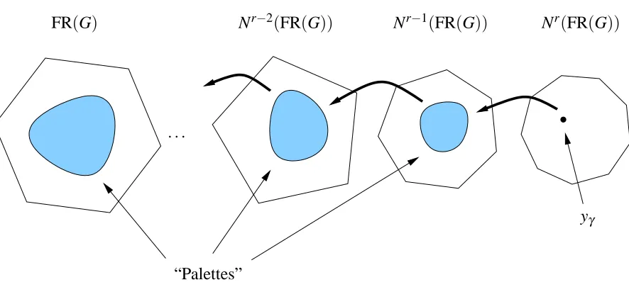
Lemma 4.1(andCorollary 4.2) suggest using induction to proveTheorem 4.5. We first will identify for each j some large set of vectors within each polytope Nj(FR(G))called the “palette” for Nj(FR(G)). In stage j of the induction we will show the following: For each vector x in the palette for Nj(FR(G)), there exists a protection matrix Y such that for all i∈[n]the vectors Yei and Y(e0−ei) all lie in the
“Palettes”
N
r−1(
FR
(
G
))
N
r−2(
FR
(
G
))
. . .
FR
(
G
)
N
r(
FR
(
G
))
y
γFigure 1: Chain of dependencies in the proof ofTheorem 4.5: Each palette is contained in its respective polytope because some other palette is contained in the previous polytope.
Since our protection matrices will be found using LP duality, we will pick the simplest palettes possible in order to ensure that our LPs are also as simple as possible (and hence easy to analyze). To understand what desirable properties the palette vectors should have, let us look at the simpler problem of showing that yγ ∈N(FR(G))(rather than showing yγ ∈Nr(FR(G))) and make some observations
about the constraints the conditions inCorollary 4.2force upon a protection matrix for yγ.
To that end, consider the projected “columns” Yei/y(γi)and Y(e0−ei)/(1−y (i)
γ )of Y (from
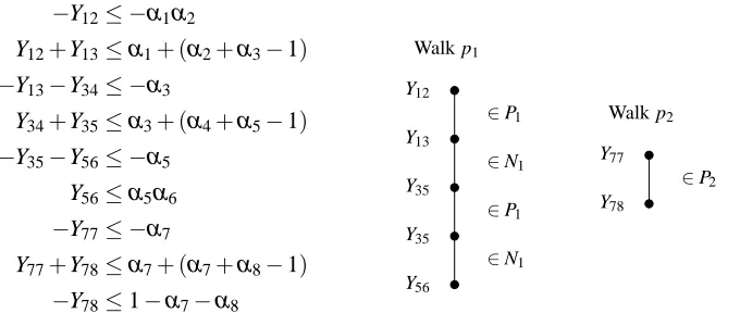
condi-tion 2 ofCorollary 4.2). These vectors must satisfy the edge constraints. As will be shown inSection 4.4 (see equation (4.14)), the constraints forcing this are given by the following constraint:
αi≤Yi j+Yik≤αi+ (αj+αk−1) ∀i∈ {1, . . . ,n},∀{j,k} ∈E . (4.12)
Fix i. If j1is adjacent to i, then (4.12) implies12+γ≤Yii+Yi j1≤ 1
2+3γ. Since Y is a protection matrix
for yγ, it must satisfy Yii=y (i)
γ = 12+γ. Hence, 0≤Yi j1 ≤2γ. Now consider a node j2 at distance
2 from j1. Then (4.12), together with the fact that 0≤Yi j1 ≤2γ for all j1 adjacent to i, imply that 1
2−γ≤Yik≤ 1
2+3γ. In turn, for a node j3 at distance 3 from i we must have 0≤Yi j3 ≤4γ; and for
a node j4 at distance 4 from i we have 12−3γ≤Yi j4 ≤ 1
2+3γ. So as j gets further and further from i,
the constraints on Yi j implied by (4.12) get looser and looser so that for nodes j sufficiently far from i
(distance 2/γmore than suffices) no constraint on Yi jis implied. So intuitively, for such j we should be
able to choose Yi j such that node j remains 12+γ in both Yei/yγ(i)and Y(e0−ei)/(1−y (i)
γ ). Note that
the fact that the coordinates of yγare 12+γinstead of 12 is crucial in ensuring that the effects of the edge
that we have simplified things by ignoring constraints required byCorollary 4.2 forcing the projected “columns” to lie in[0,1]n+1: these tighten the above constraints on the Yi j a bit but the intuition given
above is mostly unchanged.
In any case, the above suggests that to prove yγ∈N(FR(G))we could use a palette consisting of all
vectors in FR(G)which are 12+γeverywhere except perhaps on some ball of radius 2/γ in G. As such, we can add “palette constraints” to the LP defining Y forcing all nodes j distant from i to be 12+γ in both Yei/y(γi)and Y(e0−ei)/(1−y(γi)). In fact, since Y must also be symmetric, the actual constraints we
will add will force the following: for all pairs of nodes i,j with distance at least 2/γbetween them, the
jth nodes in Yei/y(γi)and Y(e0−ei)/(1−y (i)
γ ), and the ith nodes Yej/y (j)
γ and Y(e0−ej)/(1−y (j) γ )must
all be12+γ.
The proof ofTheorem 4.5will use generalized versions of the above palette: The palettes for each polytope Nj(FR(G))will consist of vectors from FR(G)that are 12+γexcept in a few neighbourhoods (seeDefinition 4.6inSection 4.2for the precise statement). For a vector x in the palette for Nj(FR(G))
the LP used to find a protection matrix Y for x will have two types of constraints: constraints that force Y to satisfy the conditions inCorollary 4.2and constraints that force the “columns” Yei/xi and Y(e0−ei)/(1−xi)to belong to the “palette” for Nj−1(FR(G)).
The palettes we will use will have the following property: The diameter of the largest neighbourhood H in G such that H consists entirely of nodes with values not equal to 12+γ will grow linearly with the number of rounds. Hence, our method is limited to proving integrality gaps for at most O(log n)rounds since only graphs with girth O(log n)yield large integrality gaps.3
4.2 Proof ofTheorem 4.5
The theorem will be proved by induction where the inductive hypothesis requires a set of vectors other than just yγ to be in Nm(FR(G)) for m≤r (the “palettes” from Section 4.1). These vectors will be
essentially all-(12+γ), except possibly for a few small neighborhoods where the vector can take arbitrary nonnegative values so long as the edge constraints are satisfied. Let Ball(w,R)denote the set of vertices within distance R of w in G.
Definition 4.6. Let S⊆ {1, . . . ,n}, R be a positive integer and γ >0. Then a nonnegative vector
(α0,α1, . . . ,αn)∈[0,1]n+1 withα0=1 is an(S,R,γ)-vector if the entries satisfy the edge constraints and if for each w∈S there exists a positive integer Rwsuch that
1. ∑w∈S(Rw+2γ)≤R
2. For distinct w,w0∈S, Ball(w,Rw)∩Ball(w0,Rw0) =/0
3. αj=12+γfor each j6∈ ∪w∈SBall(w,Rw)
We will say that the integers{Rw}w∈Switness thatαis an(S,R,γ)-vector.
Let R(r)=0 and let R(m)=R(m+1)+γ4 for 0≤m<r. Note that 4R(m)≤girth(G)for 0≤m≤r. To
proveTheorem 4.5we will prove the inductive claim below. Since the set of(/0,R(r),γ)-vectors consists precisely of the vector yγ, the theorem will then follow as a subcase of the case m=r.
Inductive Claim for Nm(FR(G)): For every set S of at most r−m vertices, every(S,R(m),γ)-vector is in Nm(FR(G)).
Base case m=0. Trivial since(S,R(0),γ)-vectors satisfy the edge constraints for G.
Proof for m+1 assuming truth for m. Let α be an(S,R(m+1),γ)-vector where |S| ≤r−m−1. To show thatα ∈Nm(FR(G)) it suffices to find a protection matrix Y for α satisfying the properties of Corollary 4.2. We exploit the structure of(S,R,γ)-vectors and prove some important structural properties of these vectors inLemma 4.7, which then enables us to argue that such a protection matrix exists thereby completing the induction step.
Note first thatα is trivially an(S∪i,R(m),γ)-vector for any i∈G.Lemma 4.7, which we now state and prove inSection 4.3below, says that for appropriate sets S0,|S0| ≤r−m,α is also an(S0,R(m),γ) -vector enjoying crucial additional structural properties.
Lemma 4.7. Let i be such thatαi 6∈ {0,1}. Then there exists a set Si⊆ {1, . . .n}, |Si| ≤r−m, and positive integers{R(wm)}w∈Si such that,
1. α is an(S0,R(m),γ)-vector with witnesses{R(wm)}w∈Si
2. i∈ ∪w∈SiBall(w,R
(m)
w )
3. For each`6∈ ∪w∈SiBall(w,R
(m)
w ), any path between i and`in G contains at least 2γ consecutive vertices`such thatα`= 12+γ
By the induction hypothesis, for any S0⊆ {1, . . . ,n}such that|S0| ≤r−m, every(S0,R(m),γ)-vector is in Nm(FR(G)). Hence, to show that α ∈Nm+1(FR(G)) it suffices byCorollary 4.2 to exhibit an (n+1)×(n+1)symmetric protection matrix Y that satisfies:
A. Ye0=diag(Y) =α,
B. For each i such thatαi=0, we have Yei =0; for each i such thatα1=1, we have Ye0 =Yei;
otherwise, Yei/αiand Y(e0−ei)/(1−αi)are(Si,R(m),γ)-vectors, where Sias well as the integers
{R(wm)}w∈Si witnessing that these vectors are(Si,R
(m),
γ)-vectors are given byLemma 4.7for i.
We will complete the proof of the induction step (and hence ofTheorem 4.5) by showing inSection 4.4 below that a matrix Y exists satisfying conditions A and B.
4.3 Proof ofLemma 4.7
Let{R(wm+1)}w∈S witness thatα is an(S,R(m+1),γ)-vector and let C=∪w∈SBall(w,R(wm+1)). There are
two cases depending on whether Ball(i,2γ)intersects C or not.
In the first (easy) case, Ball(i,2γ)does not intersect C. Then let Si =S∪ {i}, let R(im)=2γ, and let
So consider the second case where Ball(i,2γ)does intersects C. Let
T1=
w∈S : i∈Ball
w,R(wm+1)+
2
γ
.
That is, T1 consists of all points in S whose balls, slightly enlarged, contain i. Note that it may be that
i∈S, in which case i∈T1.
Now let
D= [
w∈T1
Ball
w,R(wm+1)+
2
γ
.
Since∑w∈S(R (m+1)
w +2γ)≤R(m+1)<12girth(G)−2γ, it follows that D is a tree. Let q be a longest path in D and let w1be a node in the middle of this path. Then certainly,
D⊆Ball w1,
∑
w∈T1
R(wm+1)+
2
γ !
.
We will now increase the size of this “big ball” around w1(perhaps also moving its centre in the process)
until there are no points w∈S outside the “big ball” for which Ball(w,Rw(m+1)+2γ) intersects the “big
ball”. We do this as follows: Suppose Ball(w1,∑w∈T1(R
(m+1)
w +2γ))intersects Ball(w0,Rw(m0+1)+2γ)for some w0∈S\T1. Add w0to
T1and call the new set T2. Reasoning as before, there exists w2∈G such that,
[
w∈T2
Ball
w,R(wm+1)+
2
γ
⊆Ball w2,
∑
w∈T2
R(wm+1)+
2
γ !
.
In general, at stage j if Ball(wj,∑w∈Tj(R
(m+1)
w +2γ))intersects Ball(w0,R(wm0+1)+2γ)for some w0∈S\Tj,
then add w0 to Tj, call the new set Tj+1, and find a new wj+1∈G (using again the same arguments as
before) such that,
[
w∈Tj+1
Ball
w,R(wm+1)+
2
γ
⊆Ball wj+1,
∑
w∈Tj+1
R(wm+1)+
2
γ !
.
Continue in this way until the first stage k for which no point w0 in S\Tk such that Ball(w0,R(wm0+1)+2γ)
intersects Ball(wk,∑w∈Tk(R
(m+1)
w +2γ)). Let T =Tkand u=wk.
We can now define Si and{R(wm)}w∈Si: Let Si= (S\T)∪ {u}. For w∈S\T , let R
(m)
w =R(wm+1); let
R(um)=
2
γ+w
∑
∈TR(wm+1)+
2
γ
.
Note first that
∑
w∈Si
R(wm)+
2
γ
=
∑
w∈S\T
R(wm)+
2
γ
+
R(um)+
2
γ
=
∑
w∈S\T
R(wm+1)+
2
γ
+
∑
w∈T
R(wm+1)+
2 γ +4 γ ! =
∑
w∈S
R(wm+1)+
2
γ
+4 γ
≤R(m+1)+4 γ =R
(m) .
The inequality above follows from the fact thatα is an(S,R(m+1),γ)-vector witnessed by the integers
R(wm+1). Henceα satisfies condition (1) of being an(Si,R(m),γ)-vector witnessed by the integers{R(wm)}.
Next note that by construction, Ball(u,R(um)) does not intersect ∪w∈S\TBall(w,R (m)
w ). Moreover,
sinceα is an(S,R(m+1),γ)-vector witnessed by the integers R(wm+1), it follows that
Ball(w,R(wm))∩Ball(w0,R(wm0)) =/0
for distinct w,w0 ∈S\T . Also, by construction,αj = 12+γ for all j6∈ ∪w∈SiBall(w,R
(m)
w ). Hence α
satisfies conditions (2) and (3) of being an(Si,R(m),γ)-vector witnessed by the integers{R (m) w }.
Next note that by construction, we have on one hand that
[
w∈T Ball
w,R(wm+1)+
2
γ
⊆Ball
u,R(um)−
2
γ
.
On the other hand, Ball(u,R(um))does not intersect∪w∈S\TBall(w,R (m+1)
w ). Sinceα is an(S,R(m+1),γ)
-vector witnessed by the integers R(wm+1), it thus follows from the definition of such vectors that for all
vertices k in Ball(u,R(um))\Ball(u,Ru(m)−2γ), we haveαk = 12+γ. Hence condition (3) of the lemma
holds.
Finally, condition (2) of the lemma holds since by construction i∈S
w∈TBall(w,R (m+1)
w +2γ). The
lemma follows.
4.4 Existence of Y
We will show that Y exists by representing conditions A and B as a linear program and then showing that the program is feasible. This approach was first used in [24] and subsequently in the conference version of this paper.
Our notation will assume symmetry, namely, Yi j will represent Y{i,j}. Condition A requires that:
Ykk=αk, ∀k∈ {1, . . . ,n} . (4.13)
Condition B requires that the vectors Yei/αiand Y(e0−ei)/(1−αi)are(Si,R(m),γ)-vectors. In
par-ticular, we need constraints on the variables Yi j forcing these vectors to satisfy both the edge constraints
The following constraints imply that Yei/αiand Y(e0−ei)/(1−αi)satisfy the edge constraints: For
all i∈ {1, . . . ,n}and all{j,k} ∈E:
αi≤Yi j+Yik≤αi+ (αj+αk−1) , (4.14)
To see that the above inequalities force Yei/αi and Y(e0−ei)/(1−αi) to satisfy the edge constraints
note first that Yei/αi satisfies the edge constraint for some edge{j,k}iff the jth and kth coordinates of Yei/αisum to at least 1. In equations, this requires Yi j/αi+Yik/αi≥1, or equivalentlyαi≤Yi j+Yikfor
the edge{j,k}. Similarly, the equation Yi j+Yik≤αi+ (αj+αk−1)implies that Y(e0−ei)/(1−αi)
satisfies the edge constraint for edge{j,k}.
Let(i,t)be a pair of vertices such thatαi,αt 6∈ {0,1}. Let Si⊆ {1, . . . ,n}be the set, and{R(wm)}w∈Si
the witnesses given byLemma 4.7for i. Then i,t are called a distant pair if t6∈ ∪w∈SiBall(w,R
(m)
w ). (Note
then thatαt =12+γ.) To ensure that Yei/αi and Y(e0−ei)/(1−αi)are(Si,R(m),γ)-vectors witnessed
by{R(wm)}w∈Si (as required by condition B) it suffices to ensure that the tth coordinates of Yei/αi and
Y(e0−ei)/(1−αi)are 12+γfor all distant pairs(i,t). In particular, for all such pairs,
Yit=αiαt =αi(
1
2+γ) . (4.15)
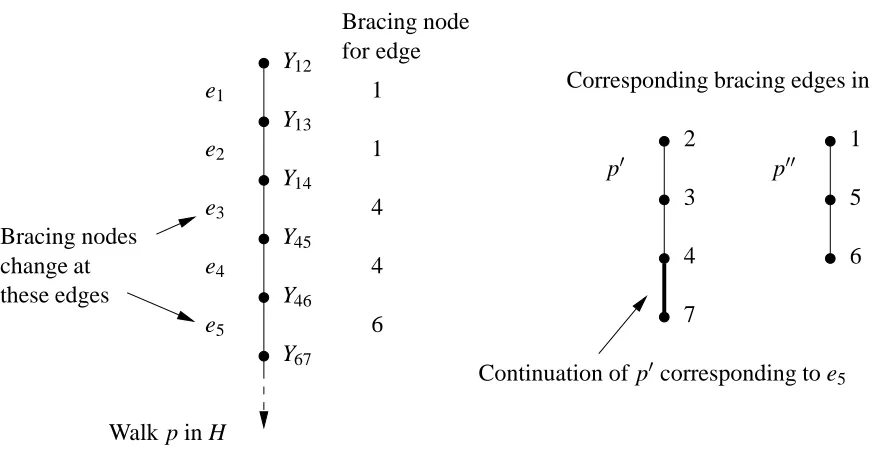
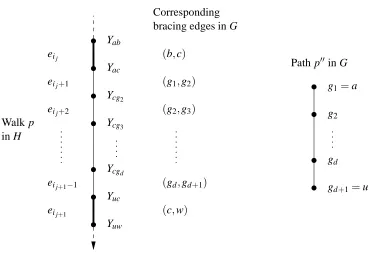
Remark 4.8. ByLemma 4.7, distant pairs have the property that every path in G that connects them contains at least 2/γconsecutive vertices k such that αk= 12+γ. In particular, any such path contains 2/γ−1 consecutive edges whose endpoints are “oversatisfied” byαby 2γ.
Finally, (Si,R(m),γ)-vectors must lie in [0,1]n+1. The following constraints imply that Yei/αi and Y(e0−ei)/(1−αi)are in[0,1]n+1:
0≤Yi j≤αi, ∀i,j∈ {1, . . . ,n},i6=j (4.16)
−Yi j≤1−αi−αj, ∀i,j∈ {1, . . . ,n},i6=j (4.17)
Constraints (4.13)–(4.17) suffice to force Y to satisfy conditions A and B. We will not directly analyze these constraints but instead analyze the following four constraint families which imply con-straints (4.13)–(4.17) but are also in a cleaner form:
Yi j≤β(i,j), ∀i,j∈ {1, . . . ,n} (4.18)
−Yi j≤δ(i,j), ∀i,j∈ {1, . . . ,n} (4.19)
Yi j+Yik≤a(i,j,k), ∀ {j,k} ∈E (4.20)
−Yi j−Yik≤b(i,j,k), ∀ {j,k} ∈E (4.21)
Here (1)β(i,j) =αiαj if i,j is a distant pair and β(i,j) =min(αi,αj) otherwise; (2)δ(i,j) =−αi
if i= j, δ(i,j) =−αiαj if i,j is a distant pair, and δ(i,j) =1−αi−αj otherwise; (3) a(i,j,k) =
αi+ (αj+αk−1); and (4) b(i,j,k) =−αi. Note that sinceα∈[0,1]n+1,β(i,j) +δ(i,j)≥0.